Magnetic Field Diagnostics Based on Far-Infrared Polarimetry: Tests Using Numerical Simulations

Abstract

The dynamical state of star-forming molecular clouds cannot be understood without determining the structure and strength of their magnetic fields. Measurements of polarized far-infrared radiation from thermally aligned dust grains are used to map the orientation of the field and estimate its strength, but the accuracy of the results has remained in doubt. In order to assess the reliability of this method, we apply it to simulated far-infrared polarization maps derived from three-dimensional simulations of supersonic magnetohydrodynamical turbulence, and compare the estimated values to the known magnetic field strengths in the simulations. We investigate the effects of limited telescope resolution and self-gravity on the structure of the maps. Limited observational resolution affects the field structure such that small scale variations can be completely suppressed, thus giving the impression of a very homogeneous field. The Chandrasekhar-Fermi method of estimating the mean magnetic field in a turbulent medium is tested, and we suggest an extension to measure the rms field. Both methods yield results within a factor of $2$ for field strengths typical of molecular clouds, with the modified version returning more reliable estimates for slightly weaker fields. However, neither method alone works well for very weak fields, missing them by a factor of up to $150$. Taking the geometric mean of both methods estimates even the weakest fields accurately within a factor of $2.5$. Limited telescope resolution leads to a systematic overestimation of the field strengths for all methods. We discuss the effects responsible for this overestimation and show how to extract information on the underlying (turbulent) power spectrum.

1 Motivation

The significance of magnetic fields in the dynamics of molecular clouds, and in star formation itself, is still uncertain.

Theory and modelling have demonstrated that the strength of magnetic fields can have a profound influence on the processes which lead to the formation of stars. There is a critical ratio of magnetic flux to mass above which magnetic fields can prevent gravitational collapse (magnetically subcritical) and below which they cannot (magnetically supercritical; e.g. Mouschovias & Spitzer 1976). Redistribution of magnetic flux by ambipolar diffusion in a magnetically subcritical region can lead to loss of support against self-gravitation, and eventually to low mass star formation (see Shu, Adams, & Lizano 1987, Myers & Goodman (1988), Porro & Silvestro (1993), Ciolek & Mouschovias 1993, 1994, 1995, Safier, McKee, & Stahler 1997, Ciolek & Königl 1998). However, magnetically subcritical regions do not appear to reproduce observations of molecular cloud cores (Nakano 1998), nor can this scenario explain the large fraction of cloud cores containing protostellar objects (Ward-Thompson, Motte, & André 1999). It is possible that magnetically supercritical regions can be supported by turbulence (Bonazzola et al. 1987, McKee & Zweibel 1995), which, to support a highly supercritical region, must be quite nonlinear (Myers & Zweibel 2001). Recent 3D simulations (Heitsch, Mac Low, & Klessen 2001, hereafter HMK, Ostriker, Stone, & Gammie 2001) demonstrate that strong turbulence can provide large-scale support against collapse, though it cannot prevent collapse on small scales. The degree to which clouds are supported at all, of course, depends on their lifetimes and on the star formation rate (Ballesteros-Paredes, Hartmann, & Vazquez-Semadeni 1999, Elmegreen 2000).

Magnetic fields affect other dynamical processes in clouds besides gravitational collapse. In a strong magnetic field, weakly compressible turbulence is anisotropic (Sridhar & Goldreich 1994; Goldreich & Sridhar 1995, 1997) and energy dissipation is relatively more in waves and less in shocks (Smith, Mac Low, & Zuev 2000), although the overall rate of energy dissipation is not strongly dependent on the fieldstrength (Mac Low 1999). Magnetic fields may also play a role in collimating molecular outflows, and in transferring their momentum to the ambient medium.

The actual strength of magnetic fields in molecular clouds will ultimately determine which theoretical picture is correct, so observations of field strengths are crucial. The integrated line of sight component of the field, weighted by the density of the tracer species, can be measured through the Zeeman effect. However, Zeeman mapping is time consuming and requires high sensitivity and the presence of particular tracers (most commonly OH). Moreover, this technique does not probe the field in the plane of the sky. For all of these reasons, it is desirable to have a complementary method of mapping the field.

Following the first detection by Cudlip et al. (1982), it has been shown that the polarization of the far infrared thermal radiation emitted by magnetically aligned dust grains can be used to map the orientation of the magnetic field on the plane of the sky (see Hildebrand et al 2000 for methodology). This has been done, at various wavelengths, for a number of nearby clouds (Gonatas et al. 1990, Jarrett et al 1994, Dotson 1996, Rao et al. 1998, Schleuning 1998, Glenn, Walker, & Young 1999, Dotson et al. 2000, Schleuning et al. 2000, Vallée, Bastien, & Greaves 2000, Ward-Thompson et al 2000) and near the Galactic Center (Werner et al. 1988, Hildebrand et al. 1990, 1993, Dowell 1997, Novak et al. 1997, 2000). Far infrared polarization maps display the morphology of the field relative to other structures in the cloud, and can also be used to estimate the strength of the mean field according to a dynamical method originally proposed by Chandrasekhar & Fermi (1953, hereafter CF). Applications of the CF-method generally suggest fieldstrengths in the milligauss range or above. Such fieldstrengths are larger than what is typically measured by the Zeeman effect (e.g. Glenn et al. 1999, Lai et al. 2000).

The CF-method is subject to errors arising from line of sight and angular averaging, and rests on the assumptions of equipartition between turbulent kinetic and magnetic energy, and isotropy of fluid motions. Spatial averaging, by smoothing the maps, can give misleading impressions about the magnetic field morphology. However, since the information carried in the maps is unique, it is difficult to test the magnitude of these effects with astronomical observations.

Numerical simulations of turbulent, magnetized molecular clouds offer the means to calibrate the accuracy of polarization maps and develop new techniques to analyze them. The actual strength and structure of the field are known at all gridpoints and at selected times, as are the gas velocity and density. It is possible to create synthetic polarization maps, analyze them as though they were astronomical data, and check the accuracy of the results. That is the subject of this paper. Ostriker, Stone, & Gammie (2001) have used a set of simulations to calibrate the CF-method in this manner.

In section 2, we describe the numerical models and the method by which we generate polarization maps. Most of the results relevant to polarization maps are in section 3, in which we discuss the morphology shown in the maps, implement the CF-method, devise an alternative to it, and show what can be learned about the spectrum of magnetic field fluctuations. Section 4 is a summary and discussion.

2 Models and Methods

2.1 Models of 3D-MHD-turbulence

We base our investigation on full 3D models of driven MHD-turbulence in a cube with periodic boundary conditions, simulating a portion of the interior of a molecular cloud. We chose an isothermal equation of state, because the cooling times are much shorter than the dynamical times at the high densities typical of molecular clouds. We performed the simulations at $128^{3}$ and $256^{3}$ grid zones resolution using ZEUS-3D, a well-tested Eulerian finite-difference code (Stone & Norman 1992a, 1992b, Clarke 1994) with second-order advection and a von Neumann artificial viscosity to capture shocks. The MHD induction equation is followed using the method of consistent transport along characteristics (Hawley & Stone 1995). We employed the massively-parallel version of the code, ZEUS-MP (Fiedler 1998, Norman 2000), to produce a data set at resolution $512^{3}$.

We used the uniform driving mechanism described in Mac Low (1999). At each timestep, a fixed pattern of velocity perturbations is added, with the amplitude adjusted such that the energy input rate is kept constant. The driving results in an rms Mach number of ${\cal M}=5$ for models of series ${\cal G}$ and of ${\cal M}=10$ for such of series ${\cal E}$ (see Table 1). The mechanism for generating the perturbation field allows us to select fixed spatial ranges. All models presented in this work employ driving at wavenumbers k=$1-2$ waves per box length $L$.

Our measurements begin at system time $t$ = 0.0, when the model has reached an equilibrium state between the energy dissipation rate due to shock interaction and numerical diffusion, and the driving energy input rate. Self-gravity is implemented via an FFT-Poisson solver for Cartesian coordinates (Burkert & Bodenheimer 1993). It is activated as soon as the model reaches the dissipation equilibrium at $t$ = 0.0.

The isothermal equation of state renders the system scale free. In code units, the length of the box is $L=2$ and the mass is $M=1$. We dimensionalize the results by choosing the Jeans length $\lambda_{J}$, Jeans mass $M_{J}$, and free fall time $t_{ff}$ (see Klessen, Heitsch, & Mac Low 2000 for discussion of the scaling). The number of Jeans masses and Jeans lengths in each run are given in Table 1.

All the models are initialized with a uniform magnetic field stretching across the box along the $z$-direction. The field becomes distorted over time, but the magnetic flux $\Phi$ through the boundaries should be constant according to the equations of ideal MHD, and is typically preserved by the code to a relative accuracy of 10^-3 - 10^-4.

As in HMK, we scale the initial magnetic fieldstrength by the plasma beta $\beta\equiv 8\pi P/B^{2}$. The parameter $\beta$ is directly related to the critical magnetic flux required to prevent global gravitational collapse (see McKee et al 1993)

$$\Phi_{c}=\frac{G^{1/2}M}{c_{\Phi}},$$ (1)

where the constant $c_{\Phi}$ is found to be 0.13 for a uniformly magnetized sphere (Mouschovias & Spitzer 1976) and 0.16 for a uniformly magnetized sheet (Nakano & Nakamura 1978). Here we choose the latter value. We find

$$\beta=8\left(\frac{\Phi_{c}}{\Phi}\frac{\lambda_{J}}{L}c_{\Phi}\right)^{2}=8\left(\frac{M}{M_{c}}\frac{\lambda_{J}}{L}c_{\Phi}\right)^{2},$$ (2)

where $M/M_{c}=\Phi_{c}/\Phi$ is the ratio of mass to critical mass as in HMK. The models discussed in this paper span the range $\beta=0.05-4.04$ and $M/M_{c}=0.88-8.3$. The Alfvén Mach number ${\cal M}_{A}$ is related to $\beta$ and the sonic Mach number ${\cal M}$ by ${\cal M}_{A}={\cal M}(\beta/2)^{1/2}$. Thus, we consider both sub-Alfvénic and super-Alfvénic models.

A detailed discussion of the model sets is given by HMK. Here we describe their physical properties just briefly. The supersonic turbulence supports the gravitationally unstable region against global collapse, however, it cannot prevent local collapse, even in the presence of magnetic fields too weak to provide magnetostatic support. Collapsing regions evolve from shock-induced filaments and cores. The models reach density contrasts of $2-3$ orders of magnitude above and below the mean density. The gravitationally bound regions can be interpreted as the initial stages of a protostellar core which may subsequently evolve into stars. Once a core begins to collapse, we cannot resolve it well enough to follow its evolution further (Truelove et al. 1997, HMK).

The isotropy of a model depends largely on its field strength. For the weak-field-model ${\cal E}h1a$, the resulting distribution of magnetic energy is fairly isotropic, whereas for the models with stronger fields (e.g. ${\cal E}h1d$), the field imprints its initial direction onto the gas flows. The flows, in turn, act on the field. Two quantities of interest for the polarization studies are the ratio of the mean field energy to the total magnetic energy, $\langle B\rangle^{2}/\langle B^{2}\rangle$, and the dispersion in the angle $\delta$ between the local magnetic field direction and the mean direction, $\sigma^{2}(\delta)$ (the two are not equivalent; for example, the energy in the field could be increased by collecting it into strong unidirectional filaments with no dispersion in angle). Both quantities are given in Table 2.

Equipartition between turbulent kinetic and turbulent magnetic energy is often assumed in astrophysics; it has been shown to hold rigorously only in certain cases, such as weak Alfvén wave turbulence (Zweibel & McKee 1995) and the incompressible Alfvénic turbulence modelled by Goldreich & Sridhar (1997). Observations do not yet yield clear evidence for or against equipartition, although data collected by Crutcher (1999) tend to speak against it. The models discussed here are not in exact equipartition; the ratio $\xi=E_{mag}^{turb}/E_{kin}$ of turbulent magnetic to turbulent kinetic energy for each model is listed in Table 2, and is typically a few tenths. It is unclear whether these departures from equipartition occur for physical reasons related to the nature of nonlinear, compressible MHD turbulence or occur because of numerical diffusivity or the nature of the forcing. We take the deviation from equipartition into account in § 3.3 to correctly interpret our polarization maps.

2.2 Generating Polarization Maps

The model cubes include density, magnetic fields and velocity fields. These data allow us to derive the Stokes parameters $Q$ and $U$, and the polarized intensity $P$ according to Zweibel (1996)

$$P=Q+iU\propto\int f(y)\frac{(B_{x}+iB_{z})^{2}}{B_{x}^{2}+B_{z}^{2}}dy$$ (3)

where $B_{x}$ and $B_{z}$ give the field vectors in the plane of sky perpendicular to the line of sight and are taken directly from the simulations. We integrate along the line of sight in $y$-direction.

The function $f(y)$ is a weighting function which accounts for the density, emissivity, and polarizing properties of the dust grains. In this paper, we take it to be the gas density normalized by the mean density. The polarized intensity is $|P|=\sqrt{Q^{2}+U^{2}}$, and the polarization angle is

$$\phi=\frac{1}{2}\arctan{\frac{Q}{U}}.$$ (4)

Equation (3) is an approximate solution of the full radiative transfer equation for the Stokes parameters (Martin 1974, Lee & Draine 1985), valid for small polarization and low optical depth. At far infrared wavelengths, and at typical column densities for molecular clouds, the medium can safely be assumed to be optically thin (Hildebrand et al. 2000).

Polarization maps are made at finite resolution. We simulate the telescope beam by applying a Gaussian filter of the form

$$F(x,x^{\prime})=\frac{1}{\sqrt{2\pi}w}\exp\left(-\frac{1}{2}\left(\frac{x-x^{\prime}}{w}\right)^{2}\right)$$ (5)

to the complex polarization $P$ given in equation (3). The width $w$ of the smoothing filter should not exceed one eighth of the box length $L$. For $w>L/8$, the tails of the filter – exceeding the map’s area – would contribute to such an extent that neglecting them would yield a too small average. For each model, we generated polarization maps with a set of smoothing widths $0\leq w\leq L/8$.

3 Results

The 2D polarization maps serve a threefold purpose: We discuss how their structure depends on self-gravity and limited observational resolution (§ 3.1), and we show that there is no preferred alignment between filamentary structures in our simulations and the magnetic fields (§ 3.2). Finally, in § 3.3 we discuss the Chandrasekhar-Fermi method of determining the mean field and an extension, which determines the rms field, both of which we test and calibrate.

3.1 Structure in Polarization Maps

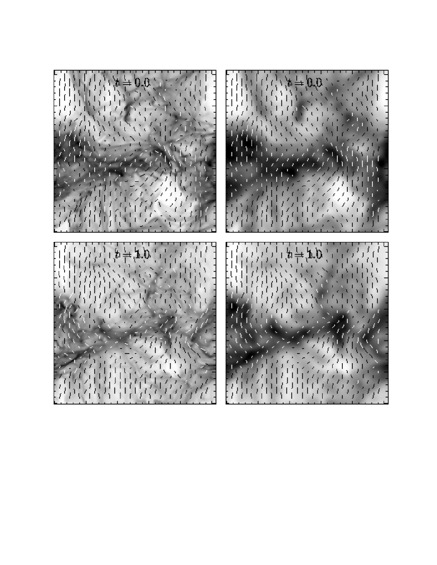
Figure 1: Left column: Surface density (corresponding to continuum density) of the full computational domain, overplotted with polarization vectors as determined by equation (3) for the self-gravitating model ${\cal E}h1d$. The magnetic field is supercritical with $M/M_{c}=1.8$. At $t=0.0$ (upper panel), gravity has been switched on, which shows its effect in the lower panel, at $t=1.0$, a free-fall time later. The initially uniform field is vertically orientated (as well as for all other maps shown). Right column: Surface density and polarization vectors as in left column, but smoothed with a Gaussian filter of $w=4$ pixel. The field gets more ordered and the previously well discernible shock structures are blurred or even come out as clumpy, filamentary structures.

The polarization maps showing column density and polarization vectors (Fig. 1 left column, model ${\cal E}h1d$) are highly structured. Shock fronts moving through the gas initiate formation of filaments and knots. After one free-fall time (lower left panel in Fig. 1), the filaments fragment and concentrate due to self-gravity. Qualitatively, no influence of self-gravity on the large-scale structure of the field is discernible, although there is some effect on the smallest scales.

Smoothing these maps with a Gaussian filter of $4$ pixels width (Fig. 1 right column, ${\cal E}h1d$) leads to a clumpier appearance of the previously well-defined filaments. Any substructure in these is lost. Single shock structures are smeared out. As expected, the field appears more uniform, thus in our case indicating more and more its initial orientation. Small scale variations in the field indicating turbulence and defining the turbulent cascade are lost due to the smoothing.

Figure 2 quantifies this effect in model ${\cal E}h1d$. It shows the power spectrum of the angle between the local and the mean magnetic field. This is equivalent to the line of sight averaged spectrum of the magnetic field fluctuation amplitude (recall that the total power in fluctuations is given in Table 2). Increasing the smoothing width from $w=0$ to $w=L/8$ results in a power loss of $96$%. Structures at a wave number of $k=8$ are suppressed by more than two orders of magnitude. The diamonds in Figure 2 indicate the power spectrum of perturbed against mean field energy $E_{mag}^{turb}/E_{mag}$, where $E_{mag}^{turb}$ is the magnetic energy corresponding to the perturbed field components perpendicular to the mean field. We use this as a measure of the true disorder in the magnetic field and as a gross check whether the polarization angles mirror the behaviour of the energies. Some power loss between the true angular dispersion and even the unsmoothed fluctuation amplitude is inevitable, because the latter involves line of sight averaging while the former is a true 3D quantity.

Inspection of Figure (1) shows no dramatic effects caused by self gravity after one free-fall time. Figure (3) shows that the width of the distribution of polarization angles does not change significantly under the effect of self-gravitation, but does certainly decrease with increasing beam width, as expected. The emerging asymmetry results from the reduced statistics due to the increasing beam width. Although every pixel contributes to the histogram, the number of independent measurements decreases with increasing beam width.

3.2 Shock-induced Filaments

There is an ongoing debate on the mechanisms generating the observed filamentary structures of molecular clouds (e.g. Loren 1989, Johnstone & Bally 1999, Matthews & Wilson 2000). Shocks come to mind as a natural explanation, either compressing the material (as in the simulations presented) or generating downstream flows resulting in the filaments (Loren 1989). The alignment of the magnetic field with the filaments has been used as a test for the validity of different filament models. The observations seem to favour no definite alignment. Maps of OMC-III (Matthews & Wilson 2000) show a perpendicular alignment, thus perhaps supporting the model of Fiege & Pudritz (2000a, 2000b), in which they propose helical fields to confine filamentary structures. Rizzo et al. (1998) found parallel and perpendicular alignment in their maps of background starlight polarization for Lupus 1 and Lupus 4, whereas Rao et al. (1998) find varying alignments for Orion-KL. Further examples of varying field alignments can be found in Dotson (1996) and Ward-Thompson et al. (2000).

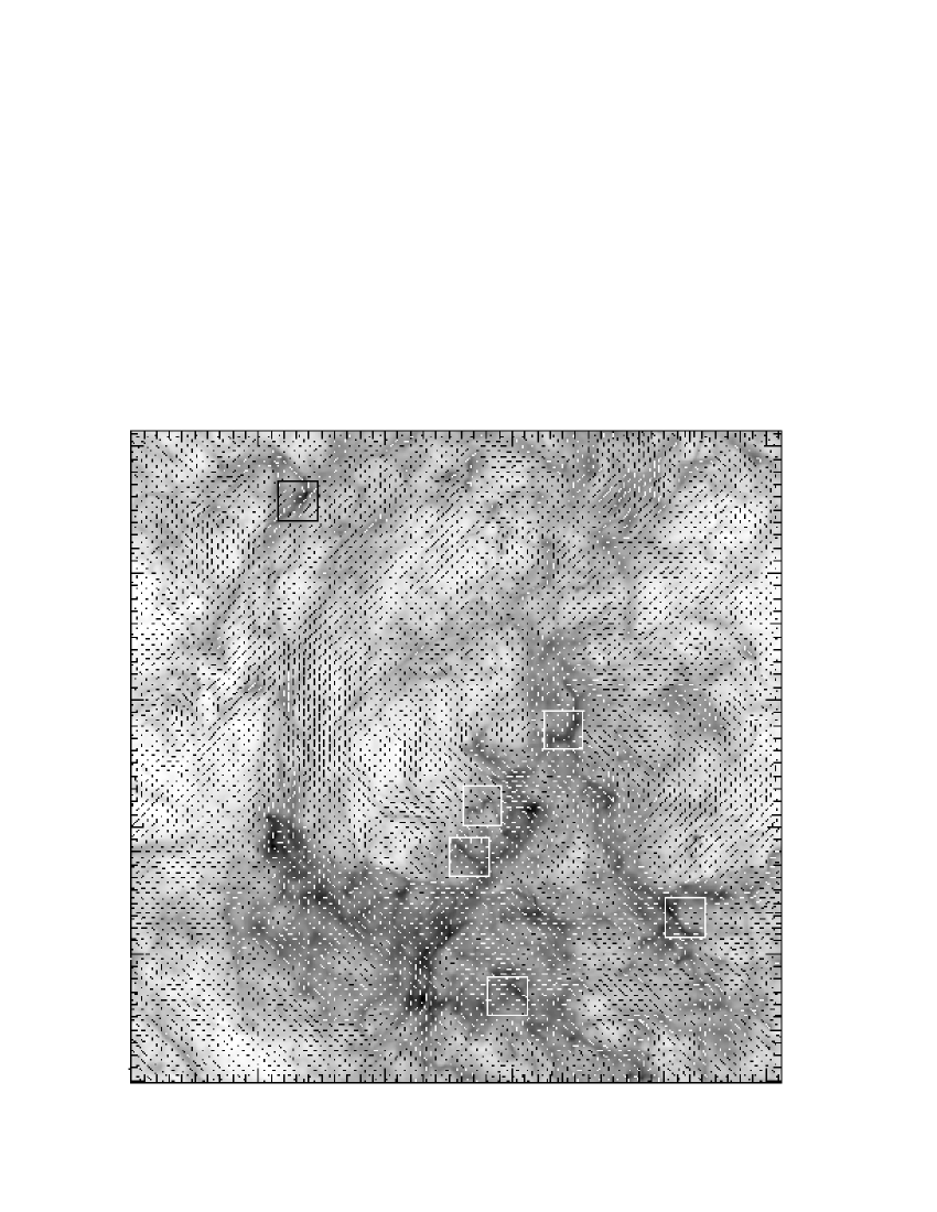
Figure 4: Surface density of the full computational domain of $512^{2}$ cells, overplotted with magnetic polarization vectors as determined by equation (3) for the not yet self-gravitating model ${\cal E}r1a$ at $t=0.0$. The magnetic field is supercritical by a factor of $8.3$. The white boxes mark the filament locations as shown in Figure 5. Every eighth polarization vector is shown.

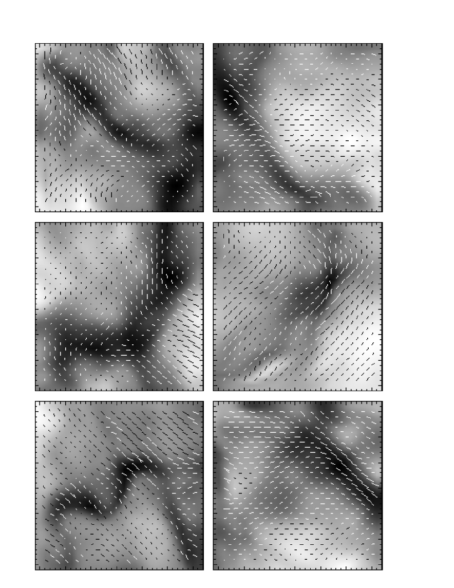
Figure 5: Magnetic polarization vectors and surface density for six selected filaments of model ${\cal E}r1a$ as denoted in Figure 4.

In the simulations presented here, the filaments are solely due to shock interactions. We do not find a preferred alignment of the magnetic field with the filaments. We illustrate this in Figure 4, which shows the full polarization map for the $512^{3}$ zone model ${\cal E}r1a$, and with a selection of filaments of the same model in Figure 5. A detailed study of the filaments will be presented in a forthcoming paper.

3.3 Estimating the Field Strength: Chandrasekhar-Fermi-Method

Chandrasekhar & Fermi (1953; CF) suggested a method of estimating the mean magnetic field strength $\langle B\rangle$ in the galactic spiral arms. It relates the line of sight velocity dispersion $\sigma(v_{los})$ to the dispersion of polarization angles $\sigma(\tan{\delta})$ around a mean field component. The CF method rests on two main assumptions: that the fluctuations are isotropic about the direction of the mean field, and that there is equipartition between the mean kinetic and magnetic energies in the fluctuations. Under these conditions, the mean field component $\langle B\rangle$ is given by

$$\langle B\rangle^{2}=4\pi\rho\frac{\sigma(v_{los})^{2}}{\sigma(\tan{\delta})^{2}}$$ (6)

where $\rho$ stands for the mean density. Because of the angular variations in the denominator, the result depends strongly on the actual mean field strength, and will in fact only be meaningful if there is a noticable mean field component. In terms of the parameter $\xi$, the ratio of turbulent magnetic to turbulent kinetic energy listed in Table 2, equation (6) generalizes to

$$\langle B\rangle^{2}=4\pi\rho\frac{\sigma(v_{los})^{2}}{\sigma(\tan{\delta})^{2}}\xi.$$ (7)

We initially set $\xi=1$ when implementing the CF-method, because observations do not yield clear evidence for or against equipartition (e.g. Crutcher 1999), but we correct for $\xi\neq 1$ later (see Table 2).

In the following paragraphs, we present a modification of the CF-method (§ 3.3.1), compare both methods with the help of model data (§ 3.3.2) and discuss the effect of limited telescope resolution on the resulting field strength estimates in § 3.3.4.

3.3.1 A Modification

The CF-method in its original form estimates the mean magnetic field. When the mean field is much less than the rms field, the dispersion in fluctuation angle $\sigma^{2}(\tan\delta)$ is dominated by points where $\delta\approx\pi/2$. Since $\langle B\rangle\propto\sigma(\tan\delta)^{-1}$ (see eq. (6)), the result is usually an underestimate of $\langle B\rangle$.

The CF-method can be extended to yield an estimate $\langle B^{2}\rangle$ which is free of this problem. Suppose $\langle B\rangle=\hat{z}\langle B\rangle$ and the $x-z$ plane is the plane of the sky. Then

$$\langle B^{2}\rangle=\langle B\rangle^{2}+\langle\Delta B_{z}^{2}\rangle+\langle B_{x}^{2}\rangle+\langle B_{y}^{2}\rangle.$$ (8)

By definition of the angle $\delta$

$$B_{x}=\langle B\rangle\tan{\delta}.$$ (9)

Squaring and averaging equation (9), assuming that the magnetic field fluctuations energies are the same for all components (see § 3.3.6), and using equation (6), equation (8) becomes

$$\langle B^{2}\rangle=4\pi\rho\frac{\sigma(v_{los})^{2}}{\sigma(\tan{\delta})^{2}}(1+3\sigma(\tan{\delta})^{2}).$$ (10)

When the field is highly disordered, and the dispersion in polarization angles is large, equation (10) reflects the underlying physical assumptions of equipartition between kinetic and magnetic energy together with isotropy. The formula is valid for arbitrary ratios of turbulent magnetic to turbulent kinetic energy if we multiply the RHS by $\xi$. When the field is highly ordered, comparison of equation (10) with equation (6) shows that the mean and rms fields are nearly the same.

3.3.2 Calibration with Model Data

We plotted the ratio of the estimated and model field strength $a\equiv B_{est}/B_{model}$ in Figure 6. The upper left panel displays $a$ for the CF-method, averaged over two lines of sight perpendicular to the mean field direction and over three physical times. The lower left panel shows the dispersion of a single measurement relative to the corresponding mean value. It decreases with increasing field strength. For strong fields, the CF-method overestimates the field strength derived from the unsmoothed maps (star symbols in Fig. 6) by a factor of $2$ to $3$. Thus we confirm the claim made by Ostriker et al. (2001). For weaker fields however, the method starts to develop a significant scatter, as shown in Figure 6 (lower panel).

The right column in Figure 6 show the corresponding results for the CF-method in its modified version according to equation (10). For the unsmoothed case (again star symbols), the strongest field is overestimated by $a\approx 3$. Whereas the original method breaks down at a field strength of $B_{model}=1.2$, the modified version still yields acceptable results for $B_{model}=0.9$.

The minimum field strength alone however does not tell us much about the reliability of the method. The parameter of interest is the Alfvén Mach number ${\cal M}_{A}=\langle v^{2}\rangle^{1/2}/c_{A}$, as the angular variations $\sigma(\tan{\delta})$ of polarization not only depend on the energy content in the field, but on the turbulent kinetic energy as well. A field strength of $B_{model}=0.9$ would correspond to ${\cal M}_{A}=1.25$, in the parameter set of models ${\cal G}$. With typical parameters of $c_{s}=200\mbox{m}/\mbox{s}$ and $n(\mbox{H}_{2})=10^{3}\mbox{ cm}^{-3}$, we can then scale $B_{model}=7\mu\mbox{G}$. Field strengths in molecular clouds are seen to be mostly larger than $B\gtrsim 10\,\mu\mbox{G}$ (Crutcher 1999). In denser regions, the field strengths seem to increase with density as $B\propto\rho^{0.47}$ (Crutcher 1999), whereas the nonthermal line widths (the “turbulence”) decreases with decreasing size as $\Delta v_{NT}\propto R^{0.21}$ (Caselli & Myers 1995). Thus we conclude, that both methods should yield acceptably accurate results for molecular cloud regions up to their densest parts, as long as the observations sample the angular variations sufficiently (see § 3.3.4).

We have to address the question of energy equipartition. Since $\xi$ is generally less than unity in our models (see Table 2), the CF-method and its extension overestimate both $\langle B\rangle$ and $\langle B^{2}\rangle$ by a factor of $1/\sqrt{\xi}$. Figure 7 shows $a\equiv B_{est}/B_{model}$ “corrected” for non-equipartition. Both methods now hit the model field strength at a factor between $1$ and $1.5$, at least for sufficiently large field strengths and for unsmoothed maps. The correction slightly reduces the largest deviations of the weak-field estimates. We conclude, that for a sufficiently well resolved (see below) polarization map and for large field strength, both methods yield reliable results. A main uncertainty factor is the ratio of magnetic to kinetic energy $\xi$ in the observed region.

Whereas the original CF-method underestimates low field strengths, the modified version overestimates them. For weak fields, the polarization angles can reach $90^{o}$ with respect to the mean field, which yields $|\tan\delta|=\infty$ in equations (6) and (10).

As the original CF-method, the modified version yields overestimated field strengths with increasing smoothing beam width. From the lower row in Figure 6 we conclude that even for the strongest fields the relative scatter is of order $20$%. Smoothing the maps leads to smaller scatter except for the weakest field strengths.

The effect of self-gravity on the field strength estimates is minute (Fig. 8). For small smoothing widths $w$, the varying small scale structure due to self-gravity leads to some statistical scatter, which is averaged out for large $w$. The CF-methods seem to be insensitive to effects of self-gravity on small scales.

3.3.3 A Recipe

The fact that $a_{CF}$ and $a_{rms}$ vary by roughly the same logarithmic range, but with opposite signs, suggests that by taking the geometric mean

$$\begin{split}a_{gm}&=\sqrt{a_{CF}\,a_{rms}}\\ &=4\pi\rho\frac{\sigma(v_{los})^{2}}{\sigma(\tan{\delta})^{2}}(1+3\sigma(\tan{\delta})^{2})^{1/2}\end{split}$$ (11)

we would arrive at a more accurate estimate for the actual field strength. Applying this recipe yields Figure 9 (corresponding to Fig. 7). Clearly, the large deviations of $a_{CF}$ and $a_{rms}$ cancel sufficiently to yield estimates accurate to a factor of $a_{gm}\approx 2.5$ even for the weakest, unsmoothed fields, and is more accurate than that for moderately strong fields. Smoothed maps of course lead again to a systematic overestimation, here up to a factor of $10$. We would like to emphasize that equation (11) is only motivated by the (logarithmically) comparable deviations of $a_{CF}$ and $a_{rms}$.

To test this recipe, we applied it to a set of models with varying physical properties (Fig. 10). Models $L1$, $L2$ and $L3$ are a time series of decaying turbulence taken from Mac Low (1999). Models $MC81$, $MA81$ and $MC41$ (Mac Low et al. 1998) are simulations of driven turbulence as series ${\cal G}$, but with driving wave length of $k=3-4$ ($MC41$) and $k=7-8$ ($MA81$, $MC81$). See Tables 1 and 2 for their parameters. All these models have weak initial fields, corresponding to ${\cal G}i1b$. As in Figure 9, the scatter of $a_{gm}$ is more than one order of magnitude lower than for $a_{CF}$ and $a_{rms}$. The unsmoothed estimates are accurate again up to a factor of $a_{gm}\approx 2.5$. Again, smoothed fields are likely to be overestimated. Note that $a_{rms}$ on the whole leads already to slightly more accurate estimates than $a_{CF}$.

We conclude that the geometric mean $a_{gm}$ gives more reliable estimates than $a_{CF}$ or $a_{gm}$ even for very weak fields, being more accurate as well for moderate and strong fields. Thus, this recipe may prove useful when being applied to observational data.

3.3.4 Smoothing, subsampling and their effect in a turbulent medium

Field estimates derived from smoothed maps tend to overestimate the field strength with increasing “beam width” (Fig. 6, all symbols except stars). We will discuss how limited telescope resolution in polarization maps of turbulent regions can lead to this overestimation.

Both CF-methods rely on perturbations of the magnetic field around a mean component. If all the power of these perturbations resided on spatial scales $1/\hat{k}=\hat{w}<w$, increasing the smoothing width above $w$ would have no effect on the power distribution of polarization angles, and varying smoothing widths would yield identical results. On the other hand, if the perturbations grew with increasing length scale, as e.g. in a turbulent power spectrum, a larger smoothing width $w$ would result in a greater power loss on larger scales, and thus to an overestimation of the field. Note that in equations (6) and (10) we find the angular variations in the denominator. So losing power in the variations increases the field estimate. The turbulence is driven between wave numbers $k=1-2$ in our simulations, thus letting the code evolve a turbulent cascade down to the dissipation scale at grid cell size. This turbulent cascade in our models is well reflected in the power spectrum of angular variations $\sigma(\delta)$ (Fig. 2). We lose more and more power when applying larger smoothing widths $w$. This power loss should depend on the steepness of the power spectrum. This suggests that it might be possible to measure the spectrum of magnetic field fluctuations by smoothing polarization maps by different filter widths, and comparing the dispersion of polarization angles.

To illustrate this relation, we will describe the smoothing as a convolution and then will determine analytically the loss of power in a spectrum due to smoothing. The convolution would be

$${\cal A}(x^{\prime})=\int_{-\infty}^{\infty}A(x)F(x-x^{\prime})\,dx$$ (12)

with the wave function $A(x)$

$$A(x)=\sum_{k=1}^{\infty}\left(\frac{1}{k}\right)^{\gamma}\sin(2\pi kx)$$ (13)

and the Gaussian filter function $F(x-x^{\prime})$ as in equation (5). We identify $A(x)$ with the $B_{x}^{2}/\langle B\rangle^{2}$ of equation (9). Instead of convolving directly, we use the Fourier transforms ${\cal F}[A]$ and ${\cal F}[F]$ of equations (13) and (5) to derive the power spectrum of the convolved function $|{\cal F}[{\cal A}]|$ via the convolution theorem

$$\hat{\cal A}=\hat{A}\hat{F},$$ (14)

where the hatted quantities denote Fourier transformations. The Fourier transform of a Gaussian yields again a Gaussian, in our case with an additional phase shift. The frequency space variable is $\omega$.

$$\begin{split}\hat{F}(\omega)&=\frac{1}{\sqrt{2\pi}w}\int_{-\infty}^{\infty}\exp\left(-\frac{1}{2}\left(\frac{x-x^{\prime}}{w}\right)^{2}\right)e^{-i\omega x}\,dx\\ &=e^{i\omega x}\,\exp\left(-\frac{1}{2}(\omega w)^{2}\right)\end{split}$$ (15)

Applying the Fourier transform to the wave function $A(x)$ and integrating over $k=[1,\infty]$, we get

$$\begin{split}\hat{A}(\omega)&=\int_{-\infty}^{\infty}\int_{k=1}^{\infty}\left(\frac{1}{k}\right)^{\gamma}\sin(2\pi kx)e^{-i\omega x}\,dk\,dx\\ &=i\pi\left(\frac{2\pi}{\omega}\right)^{\gamma}\end{split}$$ (16)

Now we can multiply $\hat{A}$ and $\hat{F}$, and taking the absolute value gives us the power spectrum of the convolved function $\cal{A}$.

$$|\hat{\cal{A}}|=\pi\exp\left(-\frac{1}{2}(\omega w)^{2}\right)\left(\frac{2\pi}{\omega}\right)^{\gamma}$$ (17)

As we are interested in the loss of power caused by the smoothing, we now try to determine the amount of power remaining in the spectrum after smoothing, i.e. the quantity

$$K(w)=\int_{0}^{\infty}\pi\,\exp\left(-\frac{1}{2}(\omega w)^{2}\right)\left(\frac{2\pi}{\omega}\right)^{\gamma}\,d\omega$$ (18)

For $\gamma\leq 1$, $\lim_{w\rightarrow 0}K(w)=\infty$. Figure 11 illustrates the behaviour of $K(w)$ for several values of $\gamma$. Note that this is a log-linear plot, so that, for example, $K(w,\gamma=3/4)\propto\log(w)^{2}$. Curves for $\gamma>1$ have negative, the ones for $\gamma<1$ positive curvature. Normalizing the curves for $\gamma<1$ with $K(0)$ and plotting them together with the inverse of the ratio of estimated to model field strength $a_{CF}$ of model ${\cal G}h1h$ yields Figure 12. We normalized $a_{CF}$ to $w=0$ as well, in order to compare the measurements to the analytic curves $K(w)$. We note that the measurements start to flatten off for small $w/L$ because of line of sight averaging, which we do not include in the analytic derivation. The same argument applies for observations. Thus, even in the ideal case of $w=0$, the measurement may not reach $a=1$ but may overestimate the actual field strength. Of course, this would crucially depend on the length of line of sight and, generally, on optical depth effects. They, however, are neglegible in the far-infrared regime. Because we need a certain length in the line of sight in order to derive a meaningful velocity dispersion $\sigma(v_{los})$, this overestimate due to line-of-sight averaging gives an intrinsic error in the CF-methods. The power spectrum of angular variations in the simulations is by no means a clear power law, due to numerical dissipation and the signatures of the driving scale. Thus, the measured $1/a_{CF}$ (Fig. 12) does not correspond clearly to one of the analytic curves. However, if observations show a well defined power law in the angular variations $\sigma(\tan{\delta})$, and provide sufficient resolution to create a series of maps smoothed over larger and larger areas, then it should be possible to extract information about the exponent of the power law and to correct the field estimate as well. Once a power law description is found for the observed region, $K(w)/K(0)$ supplies a correction factor for the field strength estimate $B_{est}$.

In polarization maps derived from observations, an additional effect could potentially lead to a systematic overestimation. When we derive the field estimates from our models, we use the complete domain, thus including all wave lengths occurring in the problem. However, it is not clear whether the observations do trace the largest scales in the field perturbations. If the power of angular variations is distributed in a power spectrum which decreases with increasing wave number, we will lose overproportionally much power when estimating the field strength within a domain which is smaller than the largest wave length contributing to the perturbations. Figure 13 illustrates this effect contributing to a systematic overestimation of the field strength. It shows the ratios $a=B_{est}/B_{model}$ for subframes of $32^{2}$, $64^{2}$ and $128^{2}$ cells for model ${\cal G}h1h$ at $256^{3}$ resolution. We averaged the estimates from all possible subframes. The error bars indicate the standard deviations of the means. With decreasing frame size, the field is overestimated slightly, thus indicating a decrease of $\sigma(\tan{\delta})$. However, bearing in mind the large scatter around the mean values in Figure 13, this effect is not very distinct.

We conclude that, although the CF-methods are applicable in principle to molecular clouds, the resulting field strengths are most likely to be systematically overestimated for two reasons: (a) Any smoothing introduced by the finite telescope beam size will lead to a systematic removal of large-scale perturbations and thus to an overestimation of the field strength. (b) Deriving field estimates for a domain smaller than the maximum perturbation wave length present leads to power loss on large scales and thus as well to an overestimated field strength. This systematic overestimation due to limited resolution is different from uncertainties because of non-equipartition as discussed in § 3.3.2. In order to draw these conclusions we assume that the underlying power spectrum of perturbations follows a power-law-like distribution, at least, that it decreases with increasing wave number.

3.3.5 Resolution Test

Figure 14 presents a test for resolution with models ${\cal G}i1h$ and ${\cal G}h1h$ at $128^{3}$ and $256^{3}$ grid cells. The beam width $w_{256}$ is given in pixels. Note that in order to compare both models, we have to compare them at the same physical beam width, i.e. we have to shift a data point of model ${\cal G}i1h$ at $w_{128}=4$ such that it corresponds to a point of $w_{256}=8$. We corrected all estimates with $1/\xi$ (see Table 2) in order to account for non-equipartition. Discrepancies at small scales are to be expected as model ${\cal G}i1h$ then already reaches the grid scale. Figure 14 allows us to conclude that numerical resolution does not affect our calibration of the CF-methods. Thus we feel justified to draw conclusions for observations of turbulent regions from our simulated observations of computational turbulence.

3.3.6 Isotropy of simulated turbulence

We still have to substantiate the claim leading to equation (8), namely, that our simulated turbulent flows are isotropic enough to validate that the field components perpendicular to the mean field $\langle B\rangle=\hat{z}\langle B\rangle$ obey $\langle B_{x}\rangle=\langle B_{y}\rangle$ and that the field perturbations in all three directions fulfill $\langle\Delta B_{z}^{2}\rangle=\langle B_{x}^{2}\rangle=\langle B_{y}^{2}\rangle$. The upper panel of Figure 15 supports the second assumption. There occur only minor differences in the rms values. Note that the initially homogeneous background field is oriented along the $z$-direction. Thus, we had to subtract this background in order to determine the corresponding mean values, yielding $\langle B_{z}\rangle$ (lower panel of Fig. 15). The scatter of the means is considerably larger, however their absolute values are three to four orders of magnitudes lower than the corresponding field strengths. Ideally, the means should vanish, especially in the directions perpendicular to the initial field, namely the $x$- and $y$-direction. Deviations from this ideal case are probably due to numerical diffusion in the code. This results in not conserving the total flux per coordinate direction. The small shifts in the means thus indicate how well the code actually does conserve the total flux.

4 Conclusions and Implications

Reliable methods for measuring and mapping magnetic fields in molecular clouds are urgently needed in order to assess the role of magnetic fields in the dynamics of molecular clouds and in star formation. Probes based on far infrared polarimetry of the thermal emission from magnetically aligned dust are now in widespread use. Far-IR polarimetry is complementary to the Zeeman method, which is the traditional means of measuring the field. There are few independent checks of its accuracy as a diagnostic of magnetic fields.

In this paper we used numerical simulations of turbulent, magnetized, self gravitating molecular clouds to assess the reliability of polarization maps. Although such simulations qualitatively reproduce many of the features seen in molecular clouds, we do not expect the computed densities, velocities, and magnetic fields to be completely realistic. We undertook the project with the expectation that analysis of simulated data would bring out the same issues as analysis of real data.

We assumed that the polarized emission is optically thin and proportional to gas density. The first assumption should be excellent. The second could be modified, for example by modelling the grain temperature point to point within the cloud. It might be possible to pick out particular structures along the line of sight by comparing maps at different wavelengths, but establishing this is beyond the scope of the present paper.

The salient properties of the models are given in Tables 1 and 2. Based on these models, our principal conclusions are as follows:

1. Filaments produced by shocks do not show a preferred alignment with the magnetic field.

2. Self-gravity has no discernible effect on the structure of the magnetic fields in our simulations. However, we have to bear mind that our self-gravitating regions are small with respect to the simulated region.

3. The Chandrasekhar-Fermi method in its original version yields field estimates accurate up to $a_{CF}=B_{CF}/\langle B\rangle=2$. A modified version determining the rms field $B_{CF}^{mod}$ results in in $a_{rms}=B_{CF}^{mod}/B_{rms}=2$. This version proves to work more reliably for slightly weaker field strengths. Both methods should be applicable to magnetic fieldstrengths typical of molecular clouds.

4. The geometrical mean $a_{gm}=\sqrt{a_{CF}\,a_{rms}}$ yields field estimates accurate up to a factor of $\approx 2.5$ even for the weakest fields. For moderate and stronger fields, $a_{gm}\approx 1$. Thus, this recipe improves the reliability of field strength estimates for the whole range of physically realistic fields in molecular clouds, and may prove useful when applied to observational data.

5. The original and modified Chandrasekhar-Fermi methods are based on the assumption of equipartition between turbulent kinetic and magnetic energy. The field fluctuations in the models are below equipartition, leading to an overestimate of the field.

6. Limited angular resolution again leads to systematic overestimation of the magnetic field strength for both methods. Two effects can cause this overestimation: (a) In a power spectrum decreasing with increasing wave number, smoothing leads to an overproportionally large power loss on larger scales. Thus the angular variations are underestimated, which leads to larger field strengths. (b) If the domain used for deriving the field estimate does not trace the largest wave modes, this again leads to power loss on the largest scales.

7. If the power spectrum of magnetic field fluctuations is a power law, field estimates made from a series of maps with different smoothing widths can in principle be used to estimate the exponent of the fluctuation spectrum, assuming that this is well enough defined over at least two decades. With this information, one could correct for the overestimated field strengths.

Table 1: Model list

Name	Resolution	$k_{drv}$	$\beta$	$M/M_{cr}$	$\lambda_{J}$	$n_{J}$
${\cal E}r1a$	$512^{3}$	$1-2$	$4.04$	$8.3$	$0.501$	$64$
${\cal E}h1a$	$256^{3}$	$1-2$	$4.04$	$8.3$	$0.501$	$64$
${\cal E}h1d$	$256^{3}$	$1-2$	$0.20$	$1.8$	$0.501$	$64$
${\cal G}i1a$	$128^{3}$	$1-2$	$4.04$	$8.3$	$1.067$	$6.5$
${\cal G}i1b$	$128^{3}$	$1-2$	$1.13$	$4.4$	$1.067$	$6.5$
${\cal G}i1c$	$128^{3}$	$1-2$	$0.50$	$2.9$	$1.067$	$6.5$
${\cal G}i1d$	$128^{3}$	$1-2$	$0.18$	$1.7$	$1.067$	$6.5$
${\cal G}i1e$	$128^{3}$	$1-2$	$0.13$	$1.5$	$1.067$	$6.5$
${\cal G}i1f$	$128^{3}$	$1-2$	$0.09$	$1.3$	$1.067$	$6.5$
${\cal G}i1g$	$128^{3}$	$1-2$	$0.07$	$1.1$	$1.067$	$6.5$
${\cal G}i1h$	$128^{3}$	$1-2$	$0.05$	$0.8$	$1.067$	$6.5$
${\cal G}h1h$	$256^{3}$	$1-2$	$0.05$	$0.8$	$1.067$	$6.5$
$L$	$256^{3}$	$1-8$	$2.00$	$\infty$	(…)	(…)
$MC81$	$128^{3}$	$7-8$	$2.00$	$\infty$	(…)	(…)
$MA81$	$128^{3}$	$7-8$	$2.00$	$\infty$	(…)	(…)
$MC41$	$128^{3}$	$3-4$	$2.00$	$\infty$	(…)	(…)

Note. — $\beta=P_{th}/P_{mag}=8\pi c_{s}^{2}\rho/B^{2}$. $M/M_{cr}$ gives the ratio of cloud mass to critical mass according to equation (1). $\lambda_{J}$ is the Jeans length, with a total box side length of $L=2$, and $n_{J}$ is the number of Jeans masses in the box. The non-selfgravitating models $L$, $MC81$, $MA81$ and $MC41$ are taken from Mac Low et al. (1998) and Mac Low (1999).

Table 2: Characteristic parameters of all models

Name	$\beta$	$\xi$	$E_{mag}/E_{kin}$	$\langle B^{2}\rangle/\langle B\rangle^{2}$	$\sigma(\delta)\,[^{o}]$
${\cal E}r1a$	$4.04$	$0.96$	$1.03$	$13.06$	$22.3$
${\cal E}h1a$	$4.04$	$0.35$	$0.37$	$12.00$	$15.0$
${\cal E}h1d$	$0.20$	$0.52$	$1.30$	$0.79$	$14.0$
${\cal G}i1a$	$4.04$	$0.21$	$0.23$	$8.90$	$20.0$
${\cal G}i1b$	$1.13$	$0.36$	$0.45$	$3.90$	$17.0$
${\cal G}i1c$	$0.50$	$0.69$	$0.91$	$3.10$	$13.0$
${\cal G}i1d$	$0.18$	$0.48$	$1.00$	$0.88$	$14.0$
${\cal G}i1e$	$0.13$	$0.31$	$1.00$	$0.45$	$13.0$
${\cal G}i1f$	$0.09$	$0.28$	$1.20$	$0.32$	$11.0$
${\cal G}i1g$	$0.07$	$0.27$	$1.30$	$0.27$	$11.0$
${\cal G}i1h$	$0.05$	$0.24$	$1.70$	$0.17$	$8.7$
${\cal G}h1h$	$0.05$	$0.26$	$2.00$	$0.15$	$9.1$
$L1$	$2.00$	$0.83$	$1.15$	$2.55$	$15.4$
$L2$	$2.00$	$1.07$	$1.78$	$1.53$	$14.4$
$L3$	$2.00$	$1.03$	$2.45$	$0.73$	$12.7$
$MC81$	$2.00$	$0.41$	$0.50$	$4.45$	$16.4$
$MA81$	$2.00$	$0.79$	$1.31$	$1.51$	$14.5$
$MC41$	$2.00$	$0.39$	$0.48$	$7.82$	$15.4$

Note. — All values are taken at $t=0.0$ except for models $L1$ to $L3$, who are a time series of decaying turbulence (Mac Low 1999). $\xi=E_{mag}^{turb}/E_{kin}$, the ratio of turbulent magnetic to turbulent kinetic energy, where $E_{mag}^{turb}$ does not include the mean ($z$-)field contribution. $E_{mag}/E_{kin}$ is the ratio of total magnetic energy (including uniform component in $z$-direction) to kinetic energy, $B^{2}_{turb}/\langle B\rangle^{2}$ is the ratio between the turbulent magnetic energy ($=E_{mag}^{turb}$) and mean field energy, and $\sigma(\delta)$ gives the dispersion of field angle around the mean field direction in degrees.

Figure 2: Power spectrum of polarization angles with respect to mean magnetic field of model ${\cal E}h1d$ and ratio $\Delta E_{mag}/E_{mag}$, corresponding to $\langle B_{x}^{2}\rangle/\langle B_{y}\rangle^{2}$, the perturbed against mean field (diamonds) against wavenumber $k$. The energy ratio is shifted horizontally by $\Delta\log(\Delta E_{mag}/E_{mag})=0.5$ for clarity. $w$ denotes the smoothing width, $0\leq w\leq L/8$, with $L=256$ the box length. At $w=L/8$, $96$% of the power in polarization angles is lost.

Figure 3: Distribution of polarization angles for two times and various smoothing beam widths $w$ of model ${\cal E}h1d$. The bottom panel starts with $t=0.0$, when gravity is switched on. The upper panel shows the angle distribution one free-fall time later. With increasing $w$, the distributions get narrower, whereas self-gravity does not affect the distributions significantly except for the smallest scales ($w=0$).

Figure 6: Overestimation factors $a_{CF}=B_{CF}/\langle B\rangle$ and $a_{rms}=B_{CF}^{mod}/B_{rms}$ for the CF-method in its original and modified version for all models of type ${\cal G}$, averaged over two lines of sight and three physical times (upper panels). The dotted lines correspond to $a=1,2,3$. Symbols stand for smoothing beams applied. Increasing beam sizes lead to systematic overestimation of the field strengths. The beam size is given in zones, with a total grid size of $128$ zones. The lower panels contain the relative standard deviations with respect to the corresponding mean value.

Figure 7: Overestimation factors $a_{CF}=B_{CF}/\langle B\rangle$ and $a_{rms}=B_{CF}^{mod}/B_{rms}$ for the CF-method in its original and modified version for all models of type ${\cal G}$ as in Figure 6, but after correcting for non-equipartition (see Table 2) with $1/\sqrt{\xi}$. The dotted lines correspond to $a=1,2,3$. Both methods return the model field strength nearly exactly for sufficiently high field strength and no smoothing.

Figure 8: Overestimation factors $a_{CF}=B_{CF}/\langle B\rangle$, $a_{rms}=B_{CF}^{mod}/B_{rms}$ and $a_{gm}=(a_{CF}a_{rms})^{1/2}$ for the self-gravitating model ${\cal E}h1d$. At $t=0.0$, gravity is switched on. Note that all three panels are plotted in the same logarithmic scale.

Figure 9: Geometric mean $a_{gm}=\sqrt{a_{CF}\,a_{rms}}$ against model field strength, averaged and corrected for non-equipartition as in Figure 7. (upper panel). Where the separate estimates $a_{CF}$ and $a_{rms}$ (Fig. 7) miss the weak field strengths by a factor $>150$ for unsmoothed ($w=0$) maps, $a_{gm}$ yields an estimate accurate up to a factor of $\approx 2.5$ for the same $w=0$-maps. Smoothed fields are still systemetically overestimated. The lower panel shows the corresponding errors.

Figure 10: $a_{CF}$, $a_{rms}$ and geometric mean $a_{gm}=\sqrt{a_{CF}\,a_{rms}}$ for an extended model set (see Table 1, lower part), corrected for non-equipartition as in Figure 7. Where the separate estimates $a_{CF}$ and $a_{rms}$ scatter around $a=1$ by up to a factor of $700$ for unsmoothed ($w=0$) values, $a_{gm}$ reduces this scatter to a factor $<10$.

Figure 11: Analytic results for the amount of power remaining in the spectrum $K(w)$ (see eq. (18)) for five values of the power law exponent $\gamma$. In this log-linear plot, exponents of $\gamma>1$ and $\gamma<1$ can be distinguished by their curvature. $L$ gives the box length.

Figure 12: Analytic results for the amount of power remaining in the spectrum $K(w)$ (see eq. (18)) for three values of the power law exponent $\gamma$. The stars denote the inverse of $a_{CF}$ taken from model ${\cal G}h1h$. All curves have been normalized to $w=0$ in order to compare them. $L$ is the box length.

Figure 13: Overestimation factors $a_{CF}=B_{CF}/\langle B\rangle$ and $a_{rms}=B_{CF}^{mod}/B_{rms}$ against linear size of subframes for model ${\cal G}h1h$. $a_{CF}$ and $a_{rms}$ were determined by averaging over all possible subframes for a given box size.

Figure 14: Overestimation factors $a_{CF}=B_{CF}/\langle B\rangle$ and $a_{rms}=B_{CF}^{mod}/B_{rms}$ against beam width $w$ for the strong-field models ${\cal G}i1h$ and ${\cal G}h1h$ at resolutions of $128^{3}$ and $256^{3}$ cells. The beam width $w_{256}$ is given in pixels, where $w_{256}$ refers to the beam width of model ${\cal G}h1h$. We have to compare the different resolutions at the same physical beam width, which is why the data points of model ${\cal G}i1h$ are shifted by a factor of $2$, i.e. $w_{128}=2\rightarrow w_{256}=4$.

Figure 15: rms field values (upper panel) and mean values (lower panel) of the magnetic fields in the three coordinate directions $x$, $y$ and $z$. The initially uniform field is parallel to the $z$-direction. For the $z$-direction, we determined the mean value after subtraction of the background field.

References

- Ballesteros-Paredes et al. (1999) Ballesteros-Paredes, J., Hartmann, L., Vazquez-Semadeni, E. 1999, ApJ, 527, 285
- Blitz & Shu (1980) Blitz, L. & Shu, F. H. 1980, ApJ, 238, 148
- Bonazzola et al. (1987) Bonazzola, S. Falgarone, E. Heyvarts, J., Perault, M. Puget, J.L. 1987, A&A, 172, 293
- Burkert & Bodenheimer (1993) Burkert, A. & Bodenheimer, P. 1993, MNRAS, 264, 798
- Caselli & Myers (1995) Caselli, P. & Myers, P.C. 1995, ApJ, 446, 665