Relativistic Jet Response to Precession and Wave-Wave Interactions

Abstract

Three dimensional numerical simulations of the response of a Lorentz factor $2.5$ relativistic jet to precession at three different frequencies have been performed. Low, moderate and high precession frequencies have been chosen relative to the maximally unstable frequency predicted by a Kelvin-Helmholtz stability analysis. Transverse motion and velocity decreases as the precession frequency increases. Although helical displacement of the jet decreases in amplitude as the precession frequency increases, a helical shock is generated in the medium external to the jet at all precession frequencies. Complex pressure and velocity structure inside the jet is shown to be produced by a combination of the helical surface and first body modes predicted by a normal mode analysis of the relativistic hydrodynamic equations. The surface and first body mode have different wave speed and wavelength, are launched in phase by the periodic precession, and exhibit beat patterns in synthetic emission images. Wave (pattern) speeds range from $0.41c$ to $0.86c$ but beat patterns remain stationary. Thus, we find a mechanism that can produce differentially moving and stationary features in the jet.

1 Introduction

Relativistic jets, particularly in extragalactic sources, can exhibit time-dependent curved structures with superluminally moving components, e.g., 3C 345 (Zensus, Cohen & Unwin 1995) or with both superluminally moving and much more slowly moving or stationary components, e.g., M 87 (Biretta, Zhou & Owen 1995; Biretta, Sparks & Macchetto 1999), 4C 39.25 (Alberdi et al. 2000), 3C 120 (Walker et al. 2001). Superluminal motions along curved trajectories can be explained by helical jet models (Hardee 1987; Steffan et al. 1995), and helical patterns are the expected result for Kelvin-Helmholtz and current driven jet instabilities in relativistic flows (Birkinshaw 1991, and references therein; Appl 1996; Istomin & Pariev 1996). It has been proposed that a combination of moving and stationary components can be the result of enhanced features moving with the jet flow through relatively fixed curved helical structures with Doppler boosting leading to fixed components where the average flow comes most nearly towards the line-of-sight (Alberdi et al. 2000; Walker et al. 2001).

Axisymmetric relativistic jet simulations have investigated component motion by introducing velocity perturbations at the origin and studying the subsequent evolution. With repeated velocity perturbations (Gomez et al. 1997; Midouszewski, Hughes & Duncan 1997) the resulting knotty structure moves with the jet flow. In a more recent axisymmetric simulation performed by Agudo et al. (2001), a single velocity perturbation generates a superluminal component associated with the velocity perturbation and multiple trailing sub-luminally moving accelerating components. These simulations address some of the issues involving components moving at different speeds but do not address the issue of components moving through stationary features or curved trajectories. To this end several 3-D hydrodynamic simulations of relativistic jets have been performed (Aloy et al. 1999; Aloy et al. 2000; Hughes et al. 1999, 2001) in which the effect of perturbation induced asymmetries on jet propagation were investigated. However, these studies did not address the issue of internal jet structure associated with asymmetric fluid motion and the component motions that might be observed inside the jets.

In this paper we present fully 3-D hydrodynamic simulations along with a detailed analysis of the time-dependent structures that develop in the jet for three different jet precession frequencies but with no velocity variation other than the relatively small transverse velocity induced by the jet precession. The numerical techniques are described in §2. Results and analysis of jet structures seen in the simulations are presented in §3 and §4. The potential observable features resulting from these structures are shown in §5, and in §6 we summarize and discuss some of the implications of our results.

2 CFD Simulations

2.1 Solution of the Euler Equations

We assume an inviscid and compressible gas, and an ideal equation of state with constant adiabatic index. We use a Godunov-type solver which is a relativistic generalization of the method of Harten, Lax, & Van Leer (1983), and Einfeldt (1988), in which the full solution to the Riemann problem is approximated by two waves separated by a piecewise constant state. We evolve the mass density $R$, the three components of the momentum density $M_{x}$, $M_{y}$ and $M_{z}$, and the total energy density $E$ relative to the laboratory frame.

Defining the vector

$$U=(R,M_{x},M_{y},M_{z},E)^{T},$$ (1)

and the three flux vectors

$$F^{x}=(Rv^{x},M_{x}v^{x}+p,M_{y}v^{y},M_{z}v^{z},(E+p)v^{x})^{T},$$ (2)

$$F^{y}=(Rv^{y},M_{x}v^{x},M_{y}v^{y}+p,M_{z}v^{z},(E+p)v^{y})^{T},$$ (3)

$$F^{z}=(Rv^{z},M_{x}v^{x},M_{y}v^{y},M_{z}v^{z}+p,(E+p)v^{z})^{T},$$ (4)

the conservative form of the relativistic Euler equation is

$${\partial{U}\over\partial{t}}+{\partial\over\partial{x}}(F^{x})+{\partial\over\partial y}(F^{y})+{\partial\over\partial z}(F^{z})=0.$$ (5)

The pressure is given by the ideal gas equation of state $p=(\Gamma-1)(e-n)$ where here and in what immediately follows we have set $c=1$. The Godunov-type solvers are well known for their capability as robust, conservative flow solvers with excellent shock capturing features. In this family of solvers one reduces the problem of updating the components of the vector $U$, averaged over a cell, to the computation of fluxes at the cell interfaces. In one spatial dimension the part of the update due to advection of the vector $U$ may be written as

$${U^{n+1}}_{i}={U^{n}}_{i}-\frac{\delta t}{\delta x}(F_{i+\frac{1}{2}}-F_{i-\frac{1}{2}}).$$ (6)

In the scheme originally devised by Godunov (1959), a fundamental emphasis is placed on the strategy of decomposing the problem into many local Riemann problems, one for each pair of values of $U_{i}$ and $U_{i+1}$ to yield values which allow the computation of the local interface fluxes $F_{i+\frac{1}{2}}$. In general, an initial discontinuity at $i+\frac{1}{2}$ due to $U_{i}$ and $U_{i+1}$ will evolve into four piecewise constant states separated by three waves. The left-most and right-most waves may be either shocks or rarefaction waves, while the middle wave is always a contact discontinuity. The determination of these four piecewise constant states can, in general, be achieved only by iteratively solving nonlinear equations. Thus the computation of the fluxes necessitates a step which can be computationally expensive. For this reason much attention has been given to approximate, but sufficiently accurate, techniques. One notable method is that of Harten, Lax, & Van Leer (1983; HLL), in which the middle wave, and the two constant states that it separates, are replaced by a single piecewise constant state. One benefit of this approximation, which smears the contact discontinuity somewhat, is to eliminate the iterative step, thus significantly improving efficiency. However, the HLL method requires accurate estimates of the wave speeds for the left- and right-moving waves. Einfeldt (1988) analyzed the HLL method and found good estimates for the wave speeds. The resulting method combining the original HLL method with Einfeldt’s improvements (the HLLE method), has been taken as a starting point for our simulations. In our implementation we use wave speed estimates based on a simple application of the relativistic addition of velocities formula for the individual components of the velocities, and the relativistic sound speed, $a$, assuming that the waves can be decomposed into components moving perpendicular to the three coordinate directions.

In order to compute the pressure $p$ and sound speed $a$ we need the rest frame mass density $n$ and energy density $e$. However, these quantities are nonlinearly coupled to the components of the velocity as well as to the laboratory frame variables via the Lorentz transformation:

$$R=\gamma n,$$ (7)

$$M^{x}=\gamma^{2}(e+p)v^{x},$$ (8)

$$M^{y}=\gamma^{2}(e+p)v^{y},$$ (9)

$$M^{z}=\gamma^{2}(e+p)v^{z},$$ (10)

$$E=\gamma^{2}(e+p)-p,$$ (11)

where $\gamma=(1-v^{2})^{-1/2}$ is the Lorentz factor and $v^{2}=(v^{x})^{2}+(v^{y})^{2}+(v^{z})^{2}$. When the adiabatic index is constant it is possible to reduce the computation of $n$, $e$, $v^{x}$, $v^{y}$ and $v^{z}$ to the solution of the following quartic equation:

$$\Bigl{[}\Gamma v\left(E-Mv\right)-M\left(1-v^{2}\right)\Bigr{]}^{2}$$

$$-\left(1-v^{2}\right)v^{2}\left(\Gamma-1\right)^{2}R^{2}=0,$$ (12)

where $M^{2}=(M^{x})^{2}+(M^{y})^{2}+(M^{z})^{2}$. This quartic is solved at each cell several times during the update of a given mesh using Newton-Raphson iteration.

Our scheme is generally of second order accuracy, which is achieved by taking the state variables as piecewise linear in each cell, and computing fluxes at the half-time step. However, in estimating the laboratory frame values on each cell boundary, it is possible that through discretization, the lab frame quantities are unphysical – they correspond to rest frame values $v>1$ or $p<0$. At each point where a transformation is needed, we check that certain conditions on $M/E$ and $R/E$ are satisfied, and if not, recompute cell interface values in the piecewise constant approximation. We find that such ‘fall back to first order’ rarely occurs.

2.2 Adaptive Mesh Refinement

The relativistic HLLE (RHLLE) method constitutes the basic flow integration scheme on a single mesh. We use adaptive mesh refinement (AMR) in order to gain spatial and temporal resolution. The AMR algorithm used is a general purpose mesh refinement scheme which is an outgrowth of original work by Berger (1982) and Berger & Colella (1989). The AMR method uses a hierarchical collection of grids consisting of embedded meshes to discretize the flow domain. We have used a scheme which subdivides the domain into logically rectangular meshes with uniform spacing in the three coordinate directions, and a fixed refinement ratio of $\times 3$. The AMR algorithm orchestrates i) the flagging of cells which need further refinement, assembling collections of such cells into meshes; ii) the construction of boundary zones so that a given mesh is a self-contained entity consisting of the interior cells and the needed boundary information; iii) mechanisms for sweeping over all levels of refinement and over each mesh in a given level to update the physical variables on each such mesh; and iv) the transfer of data between various meshes in the hierarchy, with the eventual completed update of all variables on all meshes to the same final time level. The adaption process is dynamic so that the AMR algorithm places further resolution where and when it is needed, as well as removing resolution when it is no longer required. Adaption occurs in time, as well as in space: the time step on a refined grid is less than that on the coarser grid, by the refinement factor for the spatial dimension. More time steps are taken on finer grids, and the advance of the flow solution is synchronized by interleaving the integrations at different levels. This helps prevent any interlevel mismatches that could adversely affect the accuracy of the simulation.

In order for the AMR method to sense where further refinement is needed, some monitoring function is required. In general we find that recognizing the presence of significant mass density gradients, contact surfaces, or strong shear is effective. The choice of function is determined by the part of the flow that has the most significance in a given study. For the simulations presented here the first two methods were employed, with the location of contact surfaces being found by comparing cell-to-cell pressure differences with cell-to-cell laboratory frame mass density differences. Since the tracking of shock waves is of paramount importance, a buffer ensures the flagging of extra cells at the edge of meshes, ensuring that important flow structures do not ‘leak’ out of meshes during the update of the hydrodynamic solution. The combined effect of using the RHLLE single mesh solver and the AMR algorithm results in a very efficient scheme. Where the RHLLE method is unable to give adequate resolution on a single coarse mesh the AMR algorithm places more cells, resulting in an excellent overall coverage of the computational domain.

2.3 Code Validation and Setup

The code has been validated using 1-D relativistic shock tube, 3-D relativistic shock reflection and 3-D relativistic blastwave trials (Hughes, Miller & Duncan 2001). Furthermore, the solver employed in the current code is a direct extension to 3-D (with a recast from Fortran 77 to Fortran 90) of the solver described by Duncan & Hughes (1994). Evidence for the accuracy and robustness of that code comes from, in addition to its application to test problems, the general agreement between studies performed with that code and with independently constructed codes (e.g., Martí et al. 1997).

In the simulations performed here, a ‘pre-existing’ jet flow is established across the computational volume, to represent the case in which a leading Mach disk and bow shock have passed, leaving a flow in pressure balance with a low density external (cocoon) medium – the shocked jet material. For all simulations we take the ratio of rest frame densities to be $\rho_{\mathrm{j}}/\rho_{\mathrm{x}}=10.0$ where $\rho$ is the rest frame mass density. The jet flow has $v_{\mathrm{j}}=0.9165c$ and $\gamma\equiv\left(1-\beta^{2}\right)^{-1/2}=2.5$. The value of the pressure (and thus the sound speeds inside and outside the jet) is adjusted to yield a generalized Mach number for the jet of $\gamma\beta/\gamma_{\mathrm{s}}\beta_{\mathrm{s}}=8$. Here $\gamma_{\mathrm{s}}\equiv\left(1-\beta_{\mathrm{s}}^{2}\right)^{-1/2}$ where $\beta_{\mathrm{s}}\equiv a/c$ and the sound speed, $a$ is given by

$$a\equiv\left[\frac{\Gamma p}{\rho+\frac{\Gamma}{\Gamma-1}\frac{p}{c^{2}}}\right]^{1/2}\text{ .}$$ (13)

With $\Gamma=5/3$ as the adiabatic index, the relevant sound speeds are $a_{\mathrm{x}}=0.6121c$ and $a_{\mathrm{j}}=0.2753c$.

The computational domain is $8R_{\mathrm{j}}\times 8R_{\mathrm{j}}\times 41R_{\mathrm{j}}$, with outflow boundary conditions imposed on all surfaces except the inflow plane, $z=$ constant. The inflow plane involves cells cut by the jet boundary for which state variables must be established through a volume-weighted average of the internal and external values. To avoid a ‘leakage’ of jet momentum into the ambient material, fixed, initial values are used across that entire boundary plane at every time step. Schlieren-like images of the pressure, in which the gradient is rendered on an exponential map, provide a way of exploring flow structures with a large range of linear scale and amplitude; an inspection of these images at the last time step of the computations described here reveals that the computations are free of any effects due to reflection from the domain boundaries. Three levels of refinement were admitted, and as the entire jet is fully refined by the AMR algorithm initially there are 27 of the finest level cells across the jet diameter, $2R_{\mathrm{j}}$; outside the jet courser cells are employed initially.

A precessional perturbation is applied at the inflow by imposing a transverse component of velocity with $v_{\perp}=0.01v_{\mathrm{j}}$. Simulations were performed with precessional perturbations $\omega R_{\mathrm{j}}/v_{\mathrm{j}}=$ (A) $0.40$, (B) $0.93$, (C) $2.69$. The simulations were halted after $\sim 44$ light-crossing-times for the jet radius, before development of structure had reached a quasi-steady state across the entire computational grid, when the AMR algorithm required refinement that exceeded the available computer memory.

3 Simulation Results

Prior to the data analysis we reduced data from all of the refined AMR “patches” in each relativistic simulation into uniformly spaced data. Each simulation contained roughly 300 patches at termination, with most patches at the finest grid resolution and occurring closer to the jet than the outer boundary. Since we wanted to observe the radial and azimuthal response within the jet at the finest resolution possible, our uniform grid along the transverse axes is at the finest resolution of the AMR simulations (13.5 zones/R_j). To reduce the size of the final data sets we have used a moderate scale grid (4.5 zones/R_j) along the jet axis in our uniformly spaced data. The lower resolution along the jet axis allows about 10 zones across 2R_j features in the axial direction; this length is similar to the wavelengths seen in the highest frequency simulation.

We evaluate simulation (theory) results quantitatively by taking 1-D slices through data cubes parallel to the $z$-axis at different radial distances along the transverse $x$-axis ($y$-axis for the theory) as indicated in Figure 1. For the simulation results shown in Figure 2 the $v_{x}$ and $v_{y}$ velocity components correspond to radial, $v_{r}$, and azimuthal, $v_{\phi}$, velocity components in cylindrical geometry. Axial velocities near to the jet axis show that the simulations are fully evolved out to about $30R_{\mathrm{j}}$ for the low and moderate frequency simulations and out to about $20R_{\mathrm{j}}$ for the high frequency simulation.

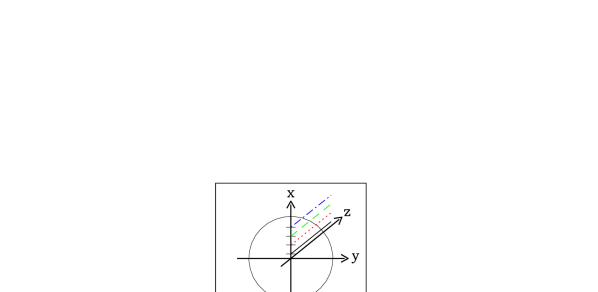
Figure 1: 1-D slices through the simulation data cubes parallel to the jet axis are located at $x/R_{\mathrm{j}}=$ (solid line) $0.11$, (dotted line) $0.33$, (dashed line) $0.55$, (dashed & dotted line) $0.77$. Similar 1-D slices through theoretical data cubes are located at similar points on the $y$-axis.

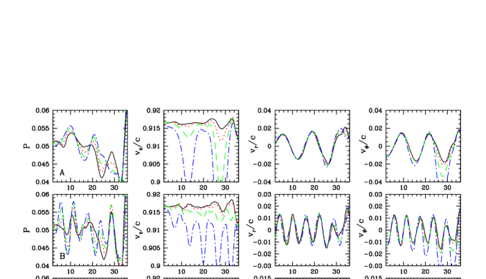
Figure 2: Pressure, axial velocity ($v_{z}$), radial velocity ($v_{x}$), and azimuthal velocity ($v_{y}$) along the 1-D slices indicated in Figure 1 for the three simulations. Line types are as in Figure 1.

Slowing of jet material resulting from surface effects is readily apparent. Surface effects penetrate more deeply into the jet as the precession frequency decreases, e.g., large dips in $v_{z}$ and $v_{\phi}$ velocity components are observed closer to the jet axis for lower precession frequency. A dominant wavelength of $\lambda/R_{\mathrm{j}}\sim$ (A) 14, (B) 6, (C) 2 is revealed in the axial velocity plots in the 1-D slices farthest from the jet axis and in the transverse velocity plots. The basic helical nature of the structure induced by precession is graphically illustrated by the out of phase oscillation in the transverse velocity components.

In all simulations the pressure structure shows oscillation clearly related to helical motion in 1-D slices farthest from the jet axis, but the structure near to the jet axis can be considerably more complicated – seen mostly in the low and moderate frequency simulations. The maximum pressure fluctuations around the local mean are less than $\pm 15\%$ and are smaller near to the jet axis and in the high frequency simulation. Growth in the transverse velocity components, indicative of unstable helical wave growth, is seen only in the low frequency simulation. In the moderate frequency simulation the transverse velocity component’s amplitude remains approximately constant. In the high frequency simulation the transverse velocity components show an initial rapid decline to a plateau. A subtle change in the radial velocity structure occurs at $z/R_{\mathrm{j}}\sim 10$ in the high frequency simulation. The change, seen in theoretical fits (see §4), occurs in the amplitude of the 1-D radial velocity slice near jet center relative to the amplitude of the 1-D slice near the jet surface. At larger distance the amplitude near to the center is less than that at the surface but at smaller distance the amplitude at center is larger. A relatively long length scale amplitude modulation of the plateau in the $v_{\phi}$ velocity component seen beyond $z/R_{\mathrm{j}}\sim 12$ in theoretical fits (see §4) may be present to a small degree in the simulation data. As we shall see in §4, subtleties like this are indicative of the presence of multiple wave modes.

Figure 3 shows a spatial Fourier analysis of the 1-D pressure, axial velocity, and radial velocity slices shown in Figure 2 but windowed from $1.888\leq z/R_{\mathrm{j}}\leq 30.111$.

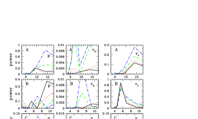
Figure 3: Spatial FFT of the pressure ($p$), axial velocity ($v_{z}$), and radial velocity ($v_{r}$) along the 1-D slices shown in Figure 2 for the three simulations. Line types are identical to Figure 2. Power associated with velocities has been normalized relative to the maximum radial velocity power and power associated with pressure has been normalized relative to the maximum in the pressure. Off the scale power is not to scale.

All velocity power amplitudes are similarly normalized with the exception of those off the scale (included so power peaks can be seen). Pressure power amplitudes are also similarly normalized. The relatively short length of our window results in coarse wavelength coverage and power is computed at $\lambda/R_{\mathrm{j}}\sim$ 28.2, 14.0, 9.3, 6.9, 5.5, 4.5, 3.8, 3.3, 2.9, 2.6, 2.4, 2.1, 2.0, 1.8, 1.7, etc. We expect power peaks to fall at the wavelength closest to the true wavelength. However, various tests indicated that shift in the location of power peaks to an adjacent wavelength bin could be caused by amplitude changes in the pressure and velocity oscillations, and also that the location of power peaks and their amplitude are somewhat sensitive to the window location. Still, it is apparent that the power distribution depends on the radial location within the jet. In general, power peaks in the radial velocity most nearly indicate the true wavelength. To a certain extent these power peaks in the radial velocity are accompanied by similar power peaks in the pressure and axial velocity at radial locations $r/R_{\mathrm{j}}=0.55$ & $0.77$. At radial locations $r/R_{\mathrm{j}}=0.11$ & $0.33$ power peaks in the pressure can be identified with similar peaks found in the axial velocity, but there are significant differences. Study of 1-D cuts through the data cubes and comparison with theoretical predictions (see §4) lead to the following general conclusions:

(1) A small amount of power in the radial velocity at wavelengths below the power peak suggests the presence of a second transverse oscillation. The effect is most evident at radial locations $r/R_{\mathrm{j}}=0.11$ & $0.33$. Power at these shorter wavelengths increases from about $1\%$ to about $10\%$ of the peak power as one goes from low to high frequency simulations. Power can also be seen to be enhanced at shorter wavelengths in pressure and axial velocity.

(2) In all simulations a significant power peak in the pressure and axial velocity, particularly apparent at radial location $r/R_{\mathrm{j}}=0.11$, occurs at $\lambda/R_{\mathrm{j}}\sim 9$. This feature can be unambiguously identified with a conical pressure wave at the inlet. This conical pressure wave appears in the 1-D pressure slices at $r/R_{\mathrm{j}}=0.11$ in Figure 2 as the pressure dip at axial distance $z/R_{\mathrm{j}}\sim 7-8$ followed by a pressure rise at $z/R_{\mathrm{j}}\sim 9-10$.

Pressure and transverse velocity vectors in planes transverse to the $z$-axis at locations of $z/R_{\mathrm{j}}=10$ & $15$ are shown in Figure 4. In these cross sections the jet flow is into the page. These locations were chosen as being far enough outwards to be relatively unaffected by inlet effects (beyond about $5R_{\mathrm{j}}$), not so far outwards as to be beyond the quasi-steady region [beyond (A & B) $30R_{\mathrm{j}}$ or (C) $20R_{\mathrm{j}}$] or where the jet surface layers are strongly slowed (beyond $20R_{\mathrm{j}}$), and to be far enough separated to see significant changes in the internal structure of the jet. The counterclockwise precession of the jet is revealed by spiral shock waves outside the jet with footpoints on low and high pressure regions on opposite sides of the jet. In the medium just outside the jet, fluid flows from high to low pressure regions around the jet circumference with less flow at higher precession frequency. The highest and lowest pressures and the largest transverse velocities lie at and outside the jet surface, but in general fluid motions in the external medium remain less than the sound speed. The existence of the spiral shocks suggests the potential for significant energy loss from the jet surface layers, and the development of a significant axial velocity shear layer and azimuthal velocity effects appears consistent with such an energy loss.

In order to see more subtle pressure and transverse velocity structure inside the jet we have applied an axial velocity mask with value $1$ if $v_{z}\geq 0.90c$ and $0$ otherwise to the cross sections.

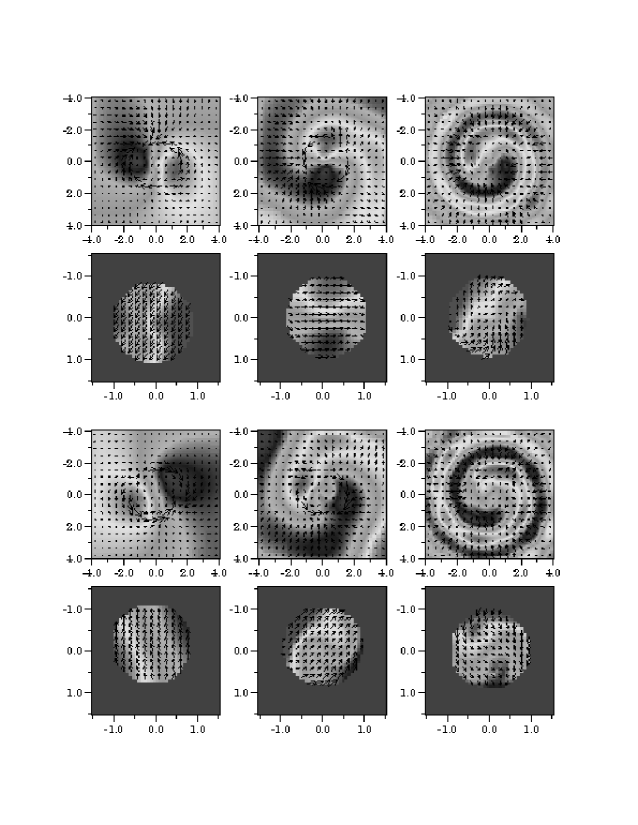
Figure 4: Transverse cross sections of the pressure structure with transverse velocity vectors superposed at axial distances $z/R_{\mathrm{j}}=$ (top six panels) $10$ & (bottom six panels) $15$. Pairs of panels show transverse structure across the entire computational grid and transverse structure masked by axial velocity to show only the jet. Low to high frequency simulation results are shown left to right. Pressure color scale and velocity vector length have been adjusted to show structure and cannot be intercompared quantitatively.

The internal pressure structure shows high and low pressure regions near to the jet surface corresponding to the high and low pressure regions beyond the jet surface in the unmasked images, but with additional complicated structure that changes dramatically between the two locations. Within the jet, transverse velocities are less than in the higher sound speed external medium. In general, transverse velocity shows jet fluid moving towards the azimuthal location of maximum jet displacement at a location farther down the jet – note that spatial rotation outwards is in the clockwise sense. This direction of transverse flow basically proceeds from the leading edge of the high pressure to leading edge of the low pressure region within the jet cross sections – recall that patterns at fixed distance rotate counterclockwise in a temporal sense. Flow patterns inside the jet show some response to internal pressure structure in the high frequency simulation but are essentially straight across the jet at the lower precession frequencies.

The complexities in internal jet structure seen in 1-D slices, as suggested by the power spectrum and by transverse cuts through the jet indicate that more is going on than can be described by a simple helical twist of the jet at one wavelength. In the next section we use all of the findings above along with a theoretical description of the normal mode structures of a cylindrical jet to identify the modes leading to the structures observed in the simulations.

4 Jet Structure

Suppose we analyze the structures arising in the simulations by modeling the jet as a cylinder of radius $R_{\mathrm{j}}$, having a uniform density, $\rho_{\mathrm{j}}$, and a uniform velocity, $v$. The external medium (cocoon) is assumed to have a uniform density, $\rho_{x}$, and to be at rest. The jet is assumed to be in static pressure balance with the external medium $p_{\mathrm{j}}=p_{x}$. A general approach to analyzing the time-dependent structures is to linearize the fluid equations along with an equation of state where the density, velocity, and pressure are written as $\rho=\rho_{0}+\rho_{1}$, ${\mathbf{v}}={\mathbf{v}}_{0}+{\mathbf{v}}_{1}$ and $p=p_{0}+p_{1}$, and subscript 1 refers to a perturbation to the equilibrium quantity. In cylindrical geometry a random perturbation of $\rho_{1}$, ${\mathbf{v}}_{1}$ and $p_{1}$ can be considered to consist of Fourier components of the form

$$f_{n}(r,\phi,z)=f_{n}(r)\exp[i(kz\pm n\phi-\omega t)]$$ (14)

where flow is along the $z$-axis, and $r$ is in the radial direction with the flow bounded by $r=R_{\mathrm{j}}$. In cylindrical geometry $k$ is the longitudinal wavenumber, $n$, is an integer azimuthal wavenumber, for $n>0$ the wave fronts propagate at an angle to the flow direction, the angle of the wavevector relative to the flow direction is $\theta=tan(n/kR)$, and $+n$ and $-n$ refer to wave propagation in the clockwise and counterclockwise senses, respectively, when viewed outward along the flow direction. The dispersion relation describing the propagation and growth of the “normal” modes, $n$, along with the expressions giving the density, pressure and velocity structure associated with the normal modes can be found in Hardee et al. (1998) and Hardee (2000).

The dispersion relation has been solved for k($\omega$) using root finding techniques for parameters appropriate to the numerical simulations. Numerical solutions to the dispersion relation for the first two pinch body modes and for the surface and first two helical body modes appropriate to the simulations are shown in Figure 5. In general, the body modes are weakly damped in a frequency range just below where they are not growing (damping rates not shown in the figure).

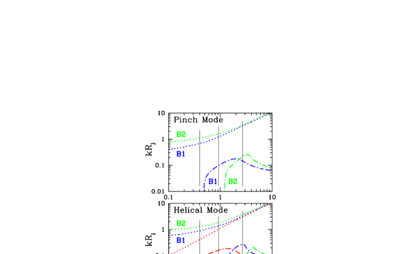
Figure 5: Numerical solution of the dispersion relation for parameters appropriate to the simulations for surface (S) wave mode or/and first two body (B₁, B₂) wave modes as a function of the angular frequency. The dotted lines give the real part of the wavenumber, $k_{R}$, and the dashed lines give the absolute value of the imaginary part of the wavenumber, $\left|k_{I}\right|$. The vertical lines indicate the precession frequency in the three numerical simulations.

The solutions have comparable maximum growth rates for these surface and body modes where the spatial growth rate is given by the imaginary part of the wavenumber, k_I. Wavelengths, wave speeds and growth (damping) lengths, $\ell\equiv|k_{I}|^{-1}$, for the helical modes at the precession frequencies used in the simulations are given in Table 1. The wave speed is defined by the real part of the phase velocity as $v_{w}=(\omega/k)|_{\mathrm{r}eal}$ and the wavelength is defined by $\lambda=2\pi v_{w}/\omega$. We note that non-relativistic jet simulations have shown wavelength and wave propagation to be given most accurately by the phase velocity and driving frequency and not, for example, by using the real part of the complex wavenumber or the group velocity to determine the wavelength. The wavelengths given in Table 1 along with mode structure and amplitudes deduced from the simulations are used to produce theoretical data cubes.

Table 1: Computed Wavelengths, Growth (damping) lengths and Wave speeds

Simulation	$\omega R_{\mathrm{j}}/v_{\mathrm{j}}$	$\lambda_{s}/R_{\mathrm{j}}$	$\ell_{s}/R_{\mathrm{j}}$	$v_{s}^{w}/c$	$\lambda_{1}/R_{\mathrm{j}}$	$\ell_{1}/R_{\mathrm{j}}$	$v_{1}^{w}/c$	$\lambda_{2}/R_{\mathrm{j}}$	$\ell_{2}/R_{\mathrm{j}}$	$v_{2}^{w}/c$
A	0.40	14.6	12.8	0.86	7.1	(119)	0.41	4.9	—	0.29
B	0.93	6.0	6.2	0.82	4.6	101	0.62	3.5	—	0.47
C	2.69	2.1	9.0	0.82	1.9	3.8	0.74	1.6	16.8	0.63

Producing theoretical data cubes that yield pressure and velocity structures similar to pressure and velocity structures in the numerical simulations was an iterative process. We concentrated on reproducing the general features seen in the simulation 1-D pressure and velocity slices (Figure 2), and then on the jet’s transverse pressure structure as shown in Figure 4. These features and structures along with the simulation power spectra shown in Figure 3 suggested the need for a pinch mode in addition to helical surface and helical body modes. This pinch contribution has been modeled by the first pinch body mode at the wavelength $\lambda_{\mathrm{p}}/R_{\mathrm{j}}=8$. This wavelength is approximately the length of the conical inlet pressure wave, is equal to the generalized Mach number, and is consistent with the power spectra shown in Figure 3. We note that the second pinch body mode exists but is not growing at this wavelength and higher order pinch body modes do not exist at this long wavelength. The 1-D radial velocity slices, which in the simulations are clearly least affected by surface effects, proved a good indicator of helical mode amplitudes. Features in the 1-D pressure slices near to the jet axis provided an indication of the relative phasing between helical surface and body modes, and, primarily in the case of the low and moderate frequency simulations, indicated the presence of pinching triggered by the conical inlet pressure wave. Fine tuning of relative phasing between modes was provided by comparing pressure structure between simulation and theoretical cross sections.

Results of a combination of helical surface and first body modes along with (A & B only) the first pinch body mode are shown as 1-D pressure and velocity slices in Figure 6.

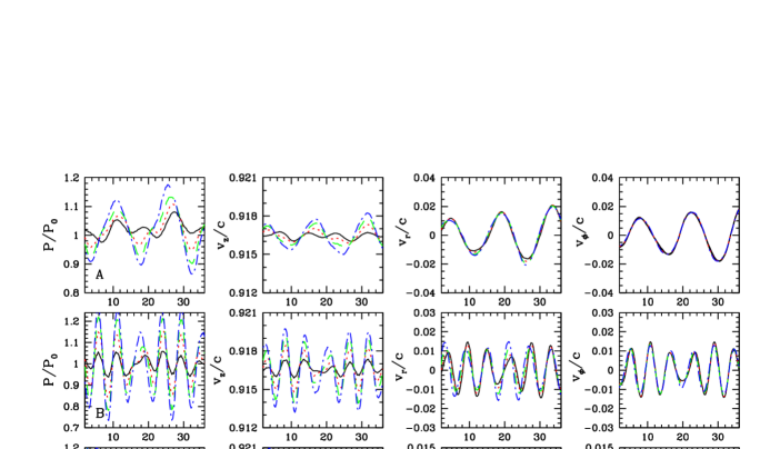
Figure 6: Pressure, axial velocity ($v_{z}$), radial velocity ($v_{y}$), and azimuthal velocity ($-v_{x}$) along 1-D slices for theoretical jet models. 1-D slice locations are now through points along the $y$-axis in Figure 1 but at the same radial locations used for the simulations. Line types are identical to Figure 2.

Qualitatively the pinch mode amplitude grows rapidly to a maximum at $z/R_{\mathrm{j}}=10$, also the approximate location of the tip of the conical pressure wave on the jet axis, and declines rapidly at larger distance, the helical surface mode amplitude grows (A) slowly with distance, (B) is constant, (C) rapidly declines to a constant value, and the helical first body mode amplitude (A) declines slowly with distance, (B) is constant, (C) grows rapidly to a constant value. Quantitatively amplitudes are input as a maximum jet surface displacement as a function of $z$, the inlet phase of the helical surface mode, $\phi_{s}$, is chosen to match the major radial velocity oscillations seen in the simulations, and the inlet phase of the helical body mode, $\phi_{1}$, is specified relative to the helical surface mode to produce interference effects and cross section structure at the appropriate locations. The inlet phase of the pinch mode is set to produce a maximum on the jet axis at $z/R_{\mathrm{j}}=10$. The expressions used for the individual modes are:

(A)

A${}_{p}=\left\{\begin{array}[]{cc}0.00075~{}z&z<10\\ 0.0075\times 2^{-(z/10-1)}&z\geq 10\end{array}\right.$

A${}_{s}=0.130+0.005~{}z$

A${}_{1}=\left\{\begin{array}[]{c}0.004\times e^{-z/120}\\ \phi_{1}=\phi_{s}+0.26\pi\end{array}\right.$

(B)

A${}_{p}=\left\{\begin{array}[]{cc}0.0004~{}z&z<10\\ 0.004\times 2^{-(z/10-1)}&z\geq 10\end{array}\right.$

A${}_{s}=0.090$

A${}_{1}=\left\{\begin{array}[]{c}0.010\\ \phi_{1}=\phi_{s}+0.5\pi\end{array}\right.$

(C)

A${}_{p}=0.0$

A${}_{s}=\left\{\begin{array}[]{cc}0.038(1-0.0770~{}z)&z<10.8\\ 0.0065&z\geq 10.8\end{array}\right.$

A${}_{1}=\left\{\begin{array}[]{cc}0.00060\times 2^{z/4}&z<13.3\\ 0.0060&z\geq 13.3\\ \phi_{1}=\phi_{s}+1.6\pi&\end{array}\right.$

where the $A$ and $z$ values above are normalized to the jet radius, $R_{\mathrm{j}}$, and $\phi_{(s,1)}$ are the phase angles at $z=0$. At the higher frequencies jet surface displacement decreases and the initial phase difference between helical surface and first body mode increases.

In general, the functional forms chosen for the amplitudes are simply a best fit to what is seen in the simulations. While amplitude growth for the pinch mode is chosen to provide a reasonable emulation of the conical pressure wave at the inlet and has no other physical significance, subsequent damping may reflect poor coupling between the conical inlet perturbation and the required structure of this pinch body mode. A similar result was found by Hardee et al. (1998) in axisymmetric relativistic jet simulations. For the first helical body mode in the low frequency precession simulation we have used the exponential damping rate predicted by the theory. Typically the helical mode wave growth or damping seen in the simulations is not exponential, e.g., slow linear growth or rapid linear damping of the surface mode in the low and high precession frequency simulations, respectively. This fact implies that amplitudes seen in the simulations are in the non-linear regime. Interestingly, the initial rapid linear damping of the helical surface mode transverse velocity components in the high frequency simulation is accompanied by rapid nearly exponential growth of oscillations in the axial velocity component. In the simulation, damping of the helical surface mode ceases when the axial velocity oscillations reach the level appropriate to the transverse velocity oscillations predicted theoretically to accompany the helical surface mode at this rapid precession frequency.

While we are able to match the major features in the 1-D slices shown in Figure 2 on the innermost 1-D slices, significant differences between theoretical and simulation 1-D slices appear in the outer half of the jet where velocity shear appears in the simulations. This velocity shear modifies the radial pressure profile, the axial velocity profile and the azimuthal velocity profile relative to the theoretical model. First, the pressure oscillations in the simulation do not attain the amplitudes seen in the theoretical profiles in the outer half of the jet. Second, the azimuthal velocity component oscillations can be greatly exaggerated in the simulations in the outer half of the jet. This second effect becomes more pronounced at lower precession frequency and at the accompanying larger sideways jet displacement. Third, a larger indication of beating between helical surface and first body modes appears in the 1-D theoretical slices. Nevertheless, results based on the linear theory appear to provide reasonable estimates of the pressure and velocity fluctuations observed in the simulations.

Theoretical transverse velocity and pressure structure of individual helical surface and first body modes at the wavelengths given in Table 1 are shown in the top six panels in Figure 7. In these panels jet flow is into the page and spatial rotation of the patterns down the jet is in a clockwise sense. At fixed position temporal rotation of the patterns is in a counterclockwise sense. For the surface mode at the fixed spatial location of the slices, transverse flow is approximately from the leading edge of the high pressure region to the leading edge of the low pressure region. Flow patterns for the first body mode at the longer wavelengths are identical and show flow towards (away from) the regions that will become high (low) pressure regions farther down the jet.

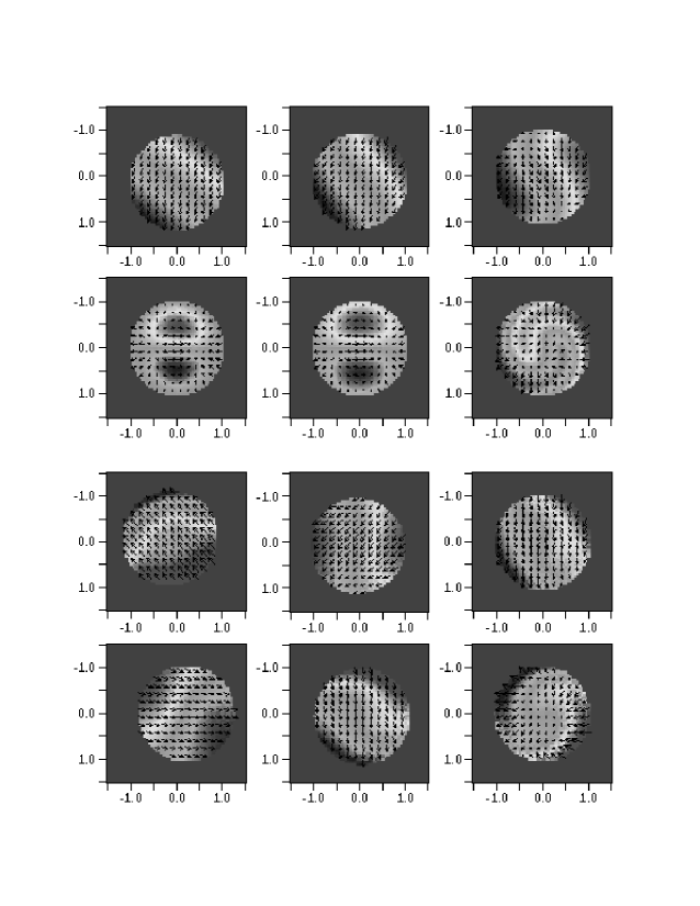
Figure 7: Transverse cross sections of the pressure structure with transverse velocity vectors superposed for individual (top row) surface and 1st body (second row) helical wave modes at (from left to right) low, moderate, and high precession frequencies. Transverse cross sections of the combined modes at axial distances (third row) $z/R_{\mathrm{j}}\sim 10$ and (bottom row ) $\sim 16,15,14$ again at the (from left to right) low, moderate, and high precession frequencies. Pressure gray scale and velocity vector length have been adjusted to show structure and cannot be intercompared quantitatively.

Results of the combined modes are shown in the bottom six panels in Figure 7. These panels show a theoretical fit to the pressure structure seen in the cross sections at $z/R_{\mathrm{j}}=10$ & $15$ in the simulations. Because we matched theoretical 1-D slices at radial positions along the transverse $y$-axis (see Figure 1) to simulation 1-D slices along the transverse $x$-axis, cross sections through the theoretical data cubes are rotated by $90^{\circ}$ relative to the simulation cross sections at comparable positions. The theoretical cross sections are taken from a theoretically generated data cube at axial locations of $z/R_{\mathrm{j}}\sim 10$ and $z/R_{\mathrm{j}}\sim$ (A) 16, (B) 15, (C) 14. Small differences in mode wavelengths between the theoretical predictions and the simulations lead to the differences in the outermost location of the best fit. We are able to reproduce the basic pressure structure seen in the simulation cross sections and the results prove that simulation structures are the result of a combination of normal modes although there are obvious differences.

In part, differences between simulation and theory are the result of the velocity shear layer that occurs in the simulations but is not included in the theoretical model. We see that transverse flow vectors are rotated relative to the pressure structure by up to about $45^{\circ}$ between theoretical cross sections and simulation cross sections. Also we find that pressure structure in the cross sections is very sensitive to the relative phasing between wave modes. For example, the theoretical cross section for simulation A at $z/R_{\mathrm{j}}\sim 10$ requires that the pinch mode provide a central pressure enhancement while the high pressure region associated with the surface and first body modes must be very close to $180^{\circ}$ out of phase. Only this phasing along with appropriate amplitudes provides a pressure cross section with characteristics similar to that of the simulation. With the exception of this cross section only the two helical modes appear important to other cross section structures. In general the body mode becomes stronger relative to the surface mode at higher precession frequency. Note that transverse velocity structure appears significantly influenced by the body mode only for the high frequency case, as in the corresponding simulation cross section.

Figure 8 shows a spatial Fourier analysis of the theoretical 1-D pressure, axial velocity, and radial velocity slices shown in Figure 6. A window from $z/R_{\mathrm{j}}\sim 2-30$ was used for low and moderate precession frequencies and $z/R_{\mathrm{j}}\sim 1-29$ was used for the high precession frequency. The length of our theoretical window and the point spacing is identical to that used for the simulations, although the normalization is different. Not surprisingly a Fourier analysis of the radial velocity slices shows the best correspondence between theory and simulation as the simulation radial velocity slices are the least influenced by surface effects. Note that relative peak power levels in the radial velocity in the three simulations are mirrored by the theoretical results. The Fourier analysis of pressure and axial velocity slices shows much more variability although similar power peaks are evident in theory and simulation results. We note that normalization, particularly for the pressure slices, is very different for theory and simulation as a result of the large difference in the amplitude of the pressure fluctuation near to the jet surface. Other differences between theory and simulation are the result of different jet structure both near and far from the inlet in the simulations. If factors such as these are considered, the Fourier analysis indicates good agreement between the theoretical models and the simulations.

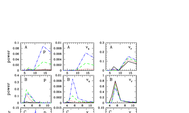
Figure 8: Spatial FFT of the pressure ($p$), axial velocity ($v_{z}$), and radial velocity ($v_{r}$) along the 1-D slices shown in Figure 6. Power associated with velocities and power associated with pressure has been normalized so that scaling is similar to that shown in Figure 3.

5 Synthetic Emission Images

The extent to which complexities in jet structure yield observable consequences is indicated by the plane of the sky line-of-sight integrations of p² shown in Figure 9. Simulation images are constructed by integrating over only those computational zones in which $v_{z}\geq 0.90c$. Intensities in the different images can be qualitatively but not quantitatively compared as the scales are not identical. Flow and pressure patterns take about $5R_{\mathrm{j}}$ to develop in the simulations so simulation and theoretical images differ on this scale. Beyond this distance simulation and theoretical images are remarkably similar.

The low frequency simulation shows a long wavelength sinusoidal oscillation at the principal wavelength indicated by the 1-D slices in Figure 2. Growth in the amplitude of oscillation is apparent in the image. Decrease in brightness along the jet in the simulation image is a manifestation of the average $15\%$ pressure drop between the inlet and $z/R_{\mathrm{j}}=30$ (see Figure 2). There is a modest enhancement in brightness where peaks appeared in the 1-D pressure slices in Figure 2 and at the locations of maximum jet displacement in the plane of the sky. The corresponding theoretical image is shifted by the expected quarter wavelength relative to the simulation image but otherwise exhibits similar structure. Modest brightness enhancement at maximum displacement is a combination of location and shape of the high pressure region within the jet and line-of-sight effects. The effect of pinch overpressure at $z/R_{\mathrm{j}}=10$ is more apparent

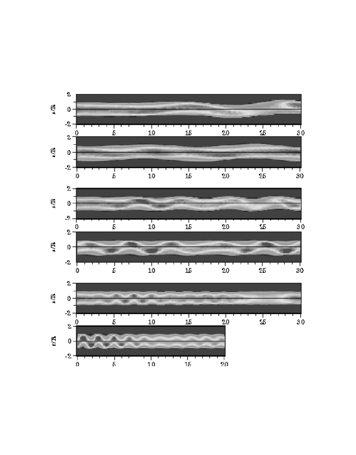
Figure 9: Line-of-sight integration of $p^{2}$ through simulation (masked by the jet velocity to show only the jet) and theoretical data cubes for low (top two panels), moderate (middle two panels) and high (bottom two panels) precession frequencies. Color scales have been adjusted to show structure and cannot be compared quantitatively.

in the theoretical image. The primary difference between the two images is a consequence of the jet’s axial pressure decline in the simulation. The presence of the helical body mode, which is at low amplitude, has no apparent influence on the appearance of the jet in simulation or theoretical images.

The moderate frequency simulation shows a sinusoidal oscillation at the principal wavelength indicated by the 1-D slices, but note the lengthening in the apparent wavelength only between $z/R_{\mathrm{j}}=14-21$. Some decrease in brightness results from an average $10\%$ pressure drop along the jet in the simulation. In this simulation significant brightness enhancement at locations of the maximum transverse displacement is apparent along much of the jet. As suggested by the 1-D velocity slices there is little growth in the oscillation amplitude. The corresponding theoretical image shows the same brightness enhancements at maximum displacement. There is more enhancement than in the low frequency images. It is readily apparent that the theoretical image reproduces the simulation image structure between $z/R_{\mathrm{j}}=14-21$. From the theoretical model we deduce that this structure is the result of interference between helical surface and first body modes.

The high frequency simulation shows two distinct sinusoidal oscillation patterns separated by a transition region centered at $z/R_{\mathrm{j}}=12-13$ although the oscillation wavelength is nearly identical on either side of the transition. A change in transverse velocity structure occurred just previous to this transition distance and can be seen in the 1-D slices in Figure 2. Similar structure is also apparent in the theoretical image and in the 1-D slices shown in Figure 6. From the theoretical model we deduce that this transition region and change in apparent structure results from decline in the helical surface mode amplitude and growth in the helical body mode amplitude and interference between the two modes. If the theoretical image is extended to larger distance with constant mode amplitudes a beat pattern emerges as a result of the slight difference in wavelength between the two wave modes. Recall that the beat pattern is apparent in the 1-D theoretical pressure and velocity slices shown in Figure 6 and also is suggested in the 1-D simulation velocity slices shown in Figure 2.

6 Summary and Discussion

In the simulations, spiral shock waves are driven into the external medium by jet helicity. While fluid motions in the external medium remain less than the sound speed the waves propagate outwards at or slightly above the sound speed. The footpoints of these waves are tied to helical “ripples” in the jet surface which move axially with speeds $0.86c>v_{z}^{w}>0.74c>a_{\mathrm{x}}=0.61c$. The azimuthal motion of the high pressure footpoint at fixed axial position increases from (A) low to (C) high precession frequency with $v_{\phi}^{w}\sim$ (A) $0.37c$, (B) $0.85c$, and (C) $2.46c$. In the high frequency simulation the high pressure footpoint moves around the jet circumference superluminally and would appear to move across the jet diameter at about $1.6c$. The existence of these spiral shocks suggests the potential for significant energy loss from the jet surface layers. In fact the simulations show the development of a significant axial velocity shear layer and azimuthal velocity effects consistent with such an energy loss. Energy loss appears greatest (as judged by axial and azimuthal velocity effects) at the low precession frequency where physical displacement of the jet surface is largest and least in the high precession frequency simulation where physical displacement of the jet surface is smallest.

Within the jet, fluid motions with respect to the helical pattern speed are less than the jet sound speed, pressure fluctuates less than $\pm 15\%$ around the local mean and velocity fluctuations in the jet fluid are much less than the jet sound speed. Axial velocity fluctuation is a very small fraction of the relativistic jet speed, and significant variation in the Lorentz factor does not occur in these relativistic jet simulations. The small transverse velocity induced by jet helicity allows for some angular variation in the flow direction. Angular variation decreases from $\pm 1.25^{\circ}$ in the low frequency simulation to about $\pm 0.3^{\circ}$ in the high frequency simulation. The angular flow variations seen in these simulations are less than 10% of the beaming angle given by $1/\gamma$ and given the relatively small variation in Lorentz factor we would not expect significant Doppler boosting fluctuations at small angles to the line-of-sight. However, we note that larger jet displacements, and larger pressure and velocity fluctuations would occur at larger distances outside the computational grid in the low frequency simulation. On the other hand, it is likely that the jet displacements, and pressure and velocity fluctuations in the high frequency simulation are close to saturation. Larger jet displacements and larger pressure and velocity fluctuations cannot be ruled out for the moderate frequency simulation beyond the length of the computational grid, although fluctuations remain relatively constant across the computational grid.

Details of internal jet pressure and velocity structure can be understood as arising from a combination of the normal modes predicted by theory. In general it is possible to provide good estimates of the velocity and pressure fluctuations in the jet interior but not near the jet surface where there is significant velocity shear in the simulations. Fitting jet structures requires a combination of helical surface and first body modes with a larger relative amplitude for first body mode as the precession frequency increases and where first body mode is more rapidly growing. Typically the helical mode wave growth or damping seen in the simulations is not exponential and this fact implies that amplitudes seen in the simulations are in the non-linear regime. Comparison with theory shows that the initial precession triggers the first helical body mode in addition to triggering the surface mode even if the body mode is not growing or is weakly damped. In the simulations some pinching is observed associated with a conical pressure wave at the inlet. The very oblique pressure wave induced at the inlet cannot couple strongly to an allowed normal pinch body wave whose structure includes a much less oblique pressure wave. Thus, we would expect damping of the initial perturbation beyond the first maximum as is suggested by theoretical fits to the simulations. A similar result was previously found by Hardee et al. (1998) for axisymmetric jets with much higher Lorentz factors.

In the line-of-sight images the sinusoidal oscillation becomes more confined to the jet interior as the precession frequency increases, and the influence of the body mode is enhanced. The high pressure region is somewhat ribbon like in cross section and this leads to enhancement in line-of-sight images at the maximum transverse displacement of the high pressure region. We note that maximum transverse displacement of the high pressure region is shifted axially relative to the maximum surface displacement. We observe additional structure within the jet in addition to the basic sinusoidal oscillation. The image structure can only be adequately understood with the modeling capability afforded by the theory. In line-of-sight images internal structure arises because of the configuration and location of the high pressure region associated primarily with the interacting helical surface and body wave modes. The modes are triggered with some initial phase difference depending on frequency but the phase difference between the modes at the inlet remains constant. In the low frequency simulation the body mode amplitude is small relative to the surface mode amplitude and there are no observable consequences of wave-wave interaction between the surface and first body mode. In the moderate and high frequency simulations where body mode amplitudes are significant, wave-wave interaction between surface and body modes does have observable consequences. In the moderate frequency simulation, line-of-sight integrations reveal the effects of constructive and destructive interference between these wave modes. In the high frequency simulation the surface mode declines and body mode grows to comparable amplitude. The image reveals interference effects similar to those seen in the moderate frequency simulation and shows that the body mode produces effects more confined to the jet interior than the surface mode. In any event we see that wave-wave interaction has observable consequences that are frequency dependent. Additionally, we find that the differences between simulation and theoretical models, particularly in the pressure fluctuations in the outer portion of the jet, do not result in significant differences in line-of-sight images.

Both simulations and theory suggest potentially interesting wave-wave interactions resulting from beating between wave modes. Since the simulations show a fixed phase difference between modes at the inlet, the different mode wavelengths result in distinct wave interaction regions (regions of constructive and destructive interference) that will remain stationary over time although individual wave patterns will move through these regions at different wave (pattern) speeds. The present simulations show that these pattern speeds can be quite different. Similar wave-wave interactions have been found also in non-relativistic numerical simulations (Xu, Hardee & Stone 2000) in a totally different parameter regime relevant to protostellar jets. Thus, this effect requires no fine tuning of parameters and should produce observable consequences on astrophysical jets in general. In the present context one might ask if the presence of moving and fixed components, or quasi-periodic spatial variation in brightness along jets indicates regions of destructive and constructive interference between normal modes excited close to the central engine. In particular, could wave-wave effects lead to the quasi-periodic spacing of brighter regions in the M 87 jet? For example, wave-wave interference could produce particularly complicated structures in a fixed or slowly moving knot, say in knot D in the M 87 jet, but with motions within the knot representative of a combination of pattern and flow speeds with very different apparent velocities. Future work will be specifically designed to address these issues.

P. Hardee, A. Rosen and E. Gomez acknowledge support from the National Science Foundation through grant AST-9802955 to the University of Alabama. P. Hughes acknowledges support from the National Science Foundation through grant AST-9617032 to the University of Michigan.

References

- (1)
- (2)
- (3) Appl, S. 1996, in ASP Conf. 100, Energy Transport in Radio Galaxies and Quasars, ed. P.E. Hardee, A.H. Bridle, & J.A. Zensus (San Francisco: ASP), 129
- (4)
- (5) Agudo, I., Gómez, J.-L., Martí, J.M., Ibáñez, J.M., Marscher, A.P., Alberdi, A., Aloy, M.-A., & Hardee, P.E. 2001, ApJL, March 10
- (6)
- (7) Alberdi, A., Gómez, J.-L., Marcaide, J.M., Marscher, A.P., Pérez-Torres, M.A. 2000, A&A, 361, 529
- (8)
- (9) Aloy, M.A., Ibáñez, J.M., Martí, J.M., Gómez, J.-L., & Müller, E. 1999, ApJ, 523, L125
- (10)
- (11) Aloy, M.A., Gómez, J.-L., Ibáñez, J.M., Martí, J.M., & Müller, E. 2000, ApJ, 528, L85
- (12)
- (13) Birkinshaw, M. 1991, in Beams and Jets in Astrophysics, ed. P.A. Hughes (Cambridge: Cambridge Univ. Press), 278
- (14)
- (15) Berger, M. 1982, Dissertation, Stanford University
- (16)
- (17) Berger, M., & Colella, P. 1989, J. Comp. Phys., 82, 67
- (18)
- (19) Biretta, J.A., Sparks, W.B., & Macchetto, F. 1999, ApJ, 520, 621
- (20)
- (21) Biretta, J.A., Zhou, F., & Owen, F.N. 1995, ApJ, 447, 582
- (22)
- (23) Duncan, G.C., & Hughes, P.A. 1994, ApJ, 436, L119
- (24)
- (25) Einfeldt, B. 1988, SIAM J. Numerical Analysis, 25, 294
- (26)
- (27) Godunov, S.K. 1959, Mat. Sb., 47, 271
- (28)
- (29) Gómez, J.-L., Martí, J.M., Marscher, A.P., Ibáñez, J.M., & Alberdi, A. 1997, ApJ, 482, L33
- (30)
- (31) Hardee, P.E. 1987, ApJ, 318, 78
- (32)
- (33) Hardee, P.E., Rosen, A., Hughes, P.A., & Duncan, G.C. 1998, ApJ, 500, 599
- (34)
- (35) Hardee, P.E. 2000, ApJ, 533, 176
- (36)
- (37) Harten, A., Lax, P., & Van Leer, B. 1983, SIAM Rev., 25, 35
- (38)
- (39) Hughes, P.A., Miller, M.A., & Duncan, G.C. 1999, BAAS, Vol.31, 1547
- (40)
- (41) Hughes, P.A., Miller, M.A., & Duncan, G.C. 2001, in preparation
- (42)
- (43) Istomin, Ya.N. & Pariev, V.I. 1996, MNRAS, 281, 1
- (44)
- (45) Martí, J.M., Müller, E., Font, J.A., Ibáñez, J.M., & Marquina, A. 1997, ApJ, 479, 151
- (46)
- (47) Mioduszewski, A.J., Hughes, P.A., & Duncan, G.C. 1997, ApJ, 476, 649
- (48)
- (49) Steffan, W., Zensus, J.A., Krichbaum, T.P., Witzel, A., & Qian, S. 1995, A&A, 302, 335
- (50)
- (51) Walker,R.C., Benson, J.M., Unwin, S.C., Lystrup, M.B., Hunter, T.R., Pilbratt, G., Hardee, P.E. 2001, ApJ, submitted
- (52)
- (53) Xu, J., Hardee, P.E., & Stone, J.M. 2000, ApJ, 543, 161
- (54)
- (55) Zensus, J.A., Cohen, M.H., & Unwin, S.C. 1995, ApJ, 443, 35
- (56)