A molecular-line study of clumps with embedded high-mass protostar candidates

We present molecular line observations made with the IRAM 30-m telescope of the immediate surroundings of a sample of 11 candidate high-mass protostars. These observations are part of an effort to clarify the evolutionary status of a set of objects which we consider to be precursors of UC Hii regions. In a preceding series of papers we have studied a sample of objects, which on the basis of their IR colours are likely to be associated with compact molecular clouds. The original sample of 260 objects was divided approximately evenly into a High group, with IR colour indices [25–12] $\geq$0.57 and [60–12] $\geq$1.3, and a Low group with complementary colours. The FIR luminosity of the Low sources, their distribution in the IR colour-colour diagram, and their lower detection rate in H₂O maser emission compared to the High sources, led to the hypothesis that the majority of these objects represent an earlier stage in the evolution than the members of the High group, which are mostly identifyable with UC Hii regions. Subsequent observations led to the selection of 12 Low sources that have FIR luminosities indicating the presence of B2.5 to O8.5 V₀ stars, are associated with dense gas and dust, have (sub-)mm continuum spectra indicating temperatures of $\sim$30 K, and have no detectable radio continuum emission. One of these sources has been proposed by us to be a good candidate for the high-mass equivalent of a Class 0 object. In the present paper we present observations of the molecular environment of 11 of these 12 objects, with the aim to derive the physical parameters of the gas in which they are embedded, and to find further evidence in support of our hypothesis that these sources are the precursors to UC Hii regions. We find that the data are consistent with such an interpretation. All observed sources are associated with well-defined molecular clumps. Masses, sizes, and other parameters depend on the tracer used, but typically the cores have average diameters of $\sim$0.5–1 pc (with a range of 0.2 to 2.2 pc), and masses of a few tens to a few thousand solar masses. Compared to a similar analysis of High sources, the present sample has molecular clumps that are more massive, larger, cooler, and less turbulent. They also tend to have a smaller ratio of virial-to-luminous mass, indicating they are less dynamically stable than their counterparts in which the High sources are embedded. The large sizes suggest these clumps should still undergo substantial contraction (their densities are $\sim$10 times smaller than those of the High sources). The lower temperatures and small linewidths are also expected in objects in an earlier evolutionary state. In various sources indications are found for outflowing gas, though its detection is hampered by the presence of multiple emission components in the line spectra. There are also signs of self-absorption, especially in the spectra of ¹³CO and HCO⁺. We find that the masses of the molecular clumps associated with our objects increase with L_fir ($\rm M_{clump}\propto L_{fir}^{1.17}$), and that there is a (weak) relation between the clump mass and the mass of the embedded protostellar object $\rm M_{proto}\propto M_{clump}^{0.30}$. The large amount of observational data is necessarily presented in a compact, reduced form. Yet we supply enough information to allow further study. These data alone cannot prove or disprove the hypothesis that among these objects a high-mass protostar is truly present. More observations, at different wavelenghts and spatial resolutions are needed to provide enough constraints on the number of possible interpretations.

1 Introduction

In spite of the importance of massive stars for the morphology and evolution of the Galaxy, and galaxies in general, the detailed study of the star formation process has mostly been concentrated on low-mass stars (M$<$1 M_⊙). The reasons for this are evident: they are more abundant than high-mass stars, and the clouds in which they form are closer by, allowing a more detailed investigation. The study of high-mass (M$\geq 10$ M_⊙) stars in their early evolutionary stages is furthermore complicated by the fact that they reach the ZAMS while still accreting material (and hence still suffering very high visual extinction), after which they rapidly destroy their natal environment.

In recent years however, ever growing efforts have been devoted to the study of the formation of high-mass stars, i.e. early type (O–B) stars with mass in excess of $\sim$ 10 M_⊙. In particular, attention has gradually shifted from the study of Hii regions to that of ultracompact (UC) Hii regions, to that of the molecular clumps in which UC Hii regions are embedded. Going from large, low-density structures to compact dense cores, corresponds to approaching the very earliest stages of the evolution of a massive star. Indeed, one of the goals of this type of research is to identify a massive stellar object in an evolutionary phase prior to the arrival on the main sequence, when most of its luminosity is derived from the release of gravitational energy. Such an object is defined a “protostar”, and would observationally be recognized as an object of Class 0 (see André et al. andre (1994)). These are most likely not to be found near UC Hii regions, because an Hii region rapidly alters (or even disrupts) the molecular cloud in which it forms. To find the initial conditions of star formation, one should therefore be looking for the precursors of UC Hii regions.

2 The search for massive protostars

The observational approach followed by our group has been illustrated in a series of papers (Palla et al. palla91 (1991), palla93 (1993); Molinari et al. molinari96 (1996), 1998a , molinari00 (2000)). A sample of 260 objects was selected from the IPSC, based on their FIR emission properties (for details see Palla et al. palla91 (1991)). In particular, the IRAS colour criteria by Richards et al. (richards (1987)) were applied, which identify compact molecular clouds. This sample was then split into two sub-samples, based on their colour indices. The 125 sources with [25$-$12] $\geq$ 0.57 and [60$-$12] $\geq$ 1.3 comply with the Wood & Churchwell (wood (1989)) criteria for identifying UC Hii regions, and are called “High”; the remaining 135 sources are called “Low”.

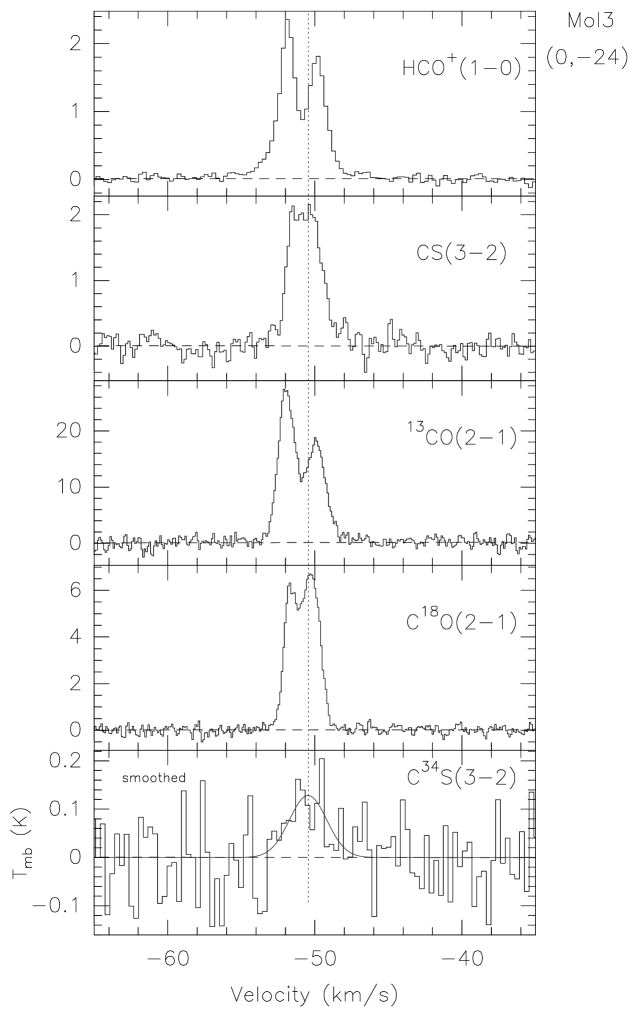
Figure 1: a Spectra towards the peak position in the maps for Mol 3. Source name, offset position, and molecules/transitions are indicated. The offset is relative to the maps’ central position, which is the sub-mm peak (Molinari et al. molinari00 (2000)). The main beam brightness temperature (T_mb) is plotted against V_lsr. The vertical dotted line indicates the V_lsr of the C³⁴S(3$-$2) line, obtained from a Gaussian fit; the horizontal dashed lines indicate the T_mb=0 K level in each spectrum.

Based on their IR properties and the H₂O maser occurrence frequency, we suggested that the Low sources are in an earlier evolutionary phase than the High sources (Palla et al. palla91 (1991)). We have then performed a series of observations with a twofold goal: to confirm that the High sources are indeed UC Hii regions, and – most importantly – to clarify the nature of the Low sources. This was accomplished by observations in many different tracers: H₂O masers (Medicina telescope), NH₃(1,1) and (2,2) lines (Effelsberg), continuum maps in the IR (ISO satellite), at centimeter (VLA), and (sub-) millimetre wavelengths (JCMT) (for a flowchart illustrating this process, see Molinari et al. molinari00 (2000), Fig. 1). The main results of these observations can be summarized as follows:

$\bullet$ High and Low sources have luminosities typical of high-mass stars, with the latter being only slightly less luminous than the former;

$\bullet$ H₂O masers are much more common towards High than Low sources (detection rates 26% and 9%, respectively);

$\bullet$ NH₃ emission is detected towards both samples (with a detection rate of 45% for Low and 80% for High sources), although the temperatures derived from the ratio of the (1,1) and (2,2) lines indicate that Low sources are slightly colder than High;

$\bullet$ Free-free emission is detected towards 43% of the High, but towards only 24% of the Low sources observed with high angular resolution with the VLA (at 2 and 6 cm);

$\bullet$ For 17 out of 30 (57%) of the Low sources mapped with the JCMT, the (sub-) millimeter continuum emission arises from a compact ($\sim$30″) region around the IRAS source; total core masses are typically 10$-$200 M_⊙;

$\bullet$ The continuum spectrum of the Low sources between 0.35 and 2 mm indicates temperatures of $\sim$30 K, significantly lower than those, measured towards “hot cores”: small ($\sim 0.1$ pc), dense ($\sim 10^{7}$ cm^-3), hot ($\gtrsim$100 K), and luminous (L$\gtrsim 10^{4}$ L_⊙) molecular condensations, which very likely host high-mass objects that are already on the main sequence, but that are still too young to have developed an UC Hii region;

The main conclusions one can draw are that High sources are UC Hii regions, and that Low sources are associated with massive stars (as suggested by their luminosities), but do not show any of the tracers typical of the molecular cores hiding a main sequence early type star (such as compact free-free emission, high kinetic temperature).

With the aim of establishing an evolutionary sequence for our sources, we have started a mapping survey with the NRAO 12-m at Kitt Peak. Two phenomena often associated with protostars (of all masses) are H₂O masers and molecular outflows. The association of CO outflows with UC Hii regions has been well established by Shepherd & Churchwell (shepherd (1996)). However, surveys show that H₂O masers can appear slightly before the development of a detectable Hii region (Codella et al. codella96 (1996), codella97 (1997)), and that they are also closely associated with CO outflows (Felli et al. felli (1992); see also Wouterloot et al. jgaw (1995), for a statistical analysis of the correlations between FIR, H₂O, and CO emission). From maps of the outflows, one can determine the dynamical timescale, which provides a lower limit to the protostellar age. Combining the presence or absence of H₂O maser- and radio continuum emission should provide a rough measure of the age of the source.

Interferometric (mm-continuum, and -lines) are needed to study the envelopes and (possible) disks of the embedded objects. Single-dish observations are important to study the physical and kinematical properties of the molecular cores, in which the candidate protostellar objects are embedded. A study of the kinematic properties is especially important: protostars derive the major part of their luminosity from accretion, and one therefore expects to see signatures of infall towards these sources (see e.g. Myers et al. myers (2000), and references therein). Although high-resolution interferometric observations are needed for a complete investigation, as a first step the resolution provided by a telescope like the IRAM 30-m will suffice to study the physical state of the sources, and to derive a rough estimate for the size and mass of the associated molecular material. Such observations are reported in the present paper.

In Sect. 3 the observations are described; the data are presented in Sect. 4. Individual sources are commented on in Sect. 5, and the results are summarized and compared with those of High sources in Sect. 6.

3 Observations

3.1 IRAM

Observations were carried out between October 10 – 12, 1997, with the IRAM 30-m telescope at Pico Veleta (Granada, Spain). We used three SIS receivers simultaneously, in combination with the 100 kHz and 1 MHz resolution filterbanks, and the autocorrelator, split into as many as five parts. The observed molecules and frequencies are listed in Table 1, where we also indicate the molecules that were observed simultaneously with the same receiver; this was achieved by tuning the receiver to a frequency intermediate between those of the two transitions.

Focus, calibration, and receiver alignment were checked by observations of Venus; the alignment was within 2″. During the observations of the program sources, pointing and calibration were checked by observations of well-known UC Hii regions and continuum sources; the rms pointing accuracy was found to be 3″, while line intensities were reproducible within 10%–20%. All line intensities in this paper are on a main beam brightness temperature (T_mb) scale.

Our sample of sources is listed in Table 2. Column 1 gives the source number from the list of Molinari et al. (molinari96 (1996)); columns 2 and 3 give the equatorial (B1950) coordinates of the central position of the maps ($\approx$ the position of the sub-mm peak as found by Molinari et al. molinari00 (2000)); columns 4 and 5 give the galactic coordinates of the IRAS source, the name of which is in column 6 ; column 7 lists the radial velocity of the NH₃(1,1) main line (from Molinari et al. molinari96 (1996)). In column 8 we give the kinematic distances (from Molinari et al. molinari00 (2000), molinari96 (1996)), while the luminosity, derived from the IRAS fluxes, and (when available) from (sub-)mm data, is given in column 9. In columns 10 to 12 we present information on the presence/absence of H₂O maser emission (from Palla et al. palla91 (1991)), radio continuum (Molinari et al. molinari96 (1996)), and a mm-detected compact core (Molinari et al. molinari00 (2000)).

We started by making small maps around the sub-mm peak position in (simultaneously) HCO⁺, ¹³CO, and CS. The initial grid size was 24″, after which we zoomed in on the peak position on a 12″ grid size. The maps were repeated several times, at least in the inner parts, in order to get a good signal-to-noise ratio. Total map extent was always $<$100″ in either direction. After having identified the peak position in this way, C¹⁸O, C³⁴S, CH₃C₂H, and CH₃CN were observed on a 3$\times$3 grid, with step size 12″, around the peak. The peak position itself was observed for up to 60 minutes in CH₃C₂H and CH₃CN. Observations were primarily done in total power mode, with an offset position 1800″ to the W; observations of CH₃C₂H and CH₃CN were done in wobbler mode, where the secondary mirror was offset by 240″.

3.2 KOSMA

In April 1999, 6 sources from Table 2 were searched for HCO⁺(4$-$3) emission ($\nu$=356734.253 MHz) with the 3-m KOSMA telescope at Gornergrat. A liquid He-cooled SIS receiver was used, and the AOS backend provided a resolution of 0.14 kms^-1. Single-pointing observations were made at the peak positions previously identified at IRAM. The KOSMA beam size was $\sim$70″$\times$78″; the beam efficiency was 0.75. Each position was observed for 15 to 30 minutes, resulting in an rms (T_mb) of 0.05$-$0.08 K. The spectra suffer from standing waves, and are therefore of rather poor quality.

4 Presentation of the data

In this section a general presentation of the available data is made, before discussing the individual sources in more detail in Sect. 5. Because of the large amount of data, a selection had to be made. In the following, we try to show a representative sample of the available observations; individual spectra and maps can be made available upon request.

4.1 Spectra at the peak positions

The spectra of HCO⁺, CS, ¹³CO, C¹⁸O and C³⁴S, taken at the peak position, are shown in Figs. 1a$-$k. The relevant parameters of these lines are collected in Table 3. In this table we give the following information: in column 1 the molecular transition; in column 2 the velocity resolution of the spectrum; the rms noise of the spectrum in column 3; in columns 4 and 5 the extreme velocities V_min, V_max where the line intensity drops below the 2$\sigma$ level; in columns 6, 7, and 8 the peak temperature, the velocity of the peak, and the FWHM line width, respectively. Because of the non-Gaussian nature of many of the line profiles, these values are read off from the spectra (as opposed to being determined from Gaussian fits); in columns 9 and 10 the values of the integral over the line, between V_min and V_max (column 9), and between the velocities where T_mb=0 K.

A comparison between the (IRAM) HCO⁺(1$-$0) and the (KOSMA) HCO⁺(4$-$3) emission is shown in Figs. 2a, b. The IRAM spectra were convolved to a 70″ beam.

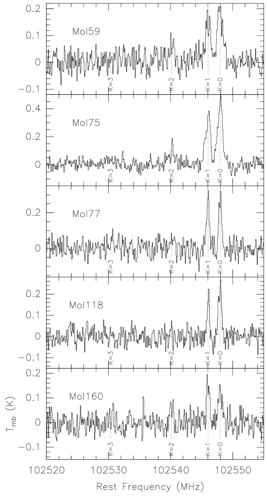
Figure 3: a Spectra of the CH₃C₂H(6$-$5) rotational transition towards the peak position. Only the higher-resolution (0.23 kms^-1) spectra are shown. The location of the first few K-components are indicated in the spectra.

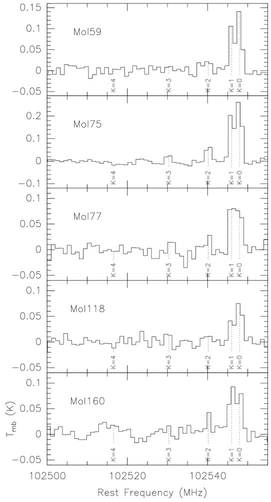
Figure 3: b As a, but for the low-resolution (2.92 kms^-1) spectra.

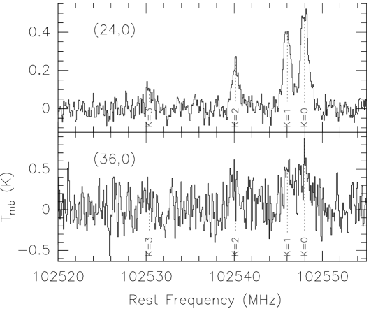
Figure 3: c As a, but for two positions towards Mol 98. The velocity resolution of the spectra is 0.23 kms^-1; the offset position at which they were taken are indicated in the panels.

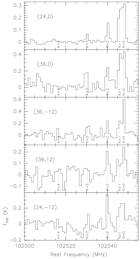
Figure 3: d As a, but for various positions towards Mol 98. The velocity resolution of the spectra is 2.92 kms^-1; the offset position at which they were taken are indicated in the panels.

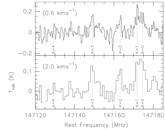
Figure 4:  Spectra of the CH₃CN(8$-$7) rotational transition towards the peak position (24″,0″) in Mol 98. The velocity resolution of the spectra is indicated in the panels. The location of the first few K-components are indicated in the spectra.

The spectra of the CH₃C₂H(6$-$5) and CH₃CN(8$-$7) detections are presented in Figs. 3a$-$d and Fig. 4, respectively. Gaussfit parameters of these lines can be found in Tables 4 and 5. When making the Gaussian fits, we fixed the velocity separation of the various K-components, and forced the widths of all K-components in a spectrum to have the same value. In none of the sources the other transitions of CH₃CN were detected, nor the CH₃OH(v_t=1) lines, which happen to lie close to the C³⁴S line.

Density-tracers, such as CS and the rare isotope C³⁴S, have been detected in all sources of our sample, implying that dense cores are indeed present. The C³⁴S lines vary in strength from a few tenths of a K, to more than 1 K; only in Mol 3 was it barely detected.

4.2 Distribution of the integrated emission

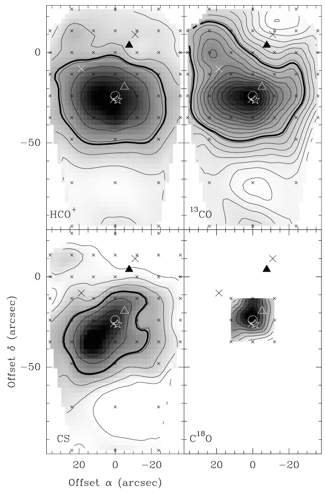
Figure 5: Maps towards all sources of the integrated emission in the lines of HCO⁺(1$-$0), ¹³CO(2$-$1), CS(3$-$2), and C¹⁸O(2$-$1). Where C³⁴S(3$-$2) was strong enough, a panel with a map of that molecule is shown as well. Thick contours indicate the 50% level in each map. The (0,0) position is the position of the sub-mm peak (Molinari et al. molinari00 (2000)). The small crosses mark the observed positions, the filled triangle indicates the IRAS point source position, and the circle marks the position where we made longer integrations at the frequency of the CH₃C₂H(6$-$5) and CH₃CN lines. a Data for Mol 3. The open triangle is the peak of the 850 $\mu$m emission, while the star indicates the position of the H₂O maser (Jenness et al. jenness (1995)). The big crosses indicate the positions of the peaks of the radio continuum emission (VLA D-array, 3.6 cm; Molinari et al. in preparation). For details, see Sect. 5. Contour values (low(step)high, in Kkms^-1) are: 0.5(1)6.5 (HCO⁺); 13(3)69 (¹³CO); 0.5(1)6.5 (CS); 9(1)17 (C¹⁸O).

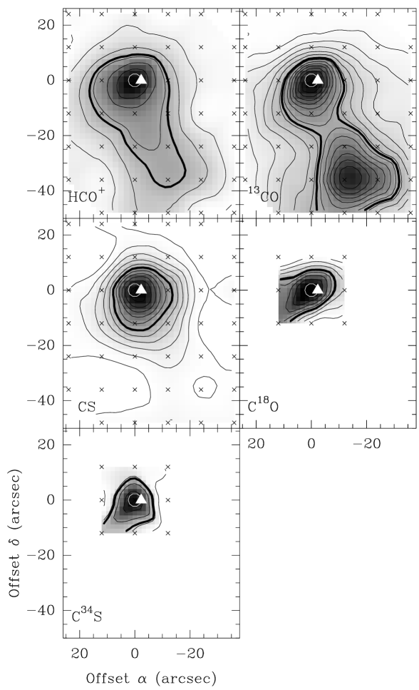
Figure 5: b Same as a, for Mol 8. Contour values (low(step)high, in Kkms^-1) are: 0.5(1)6.5 (HCO⁺); 4.5(4)60.5 (¹³CO); 0.5(1)11 (CS); 1(1)8 (C¹⁸O); 0.4(0.4)2 (C³⁴S).

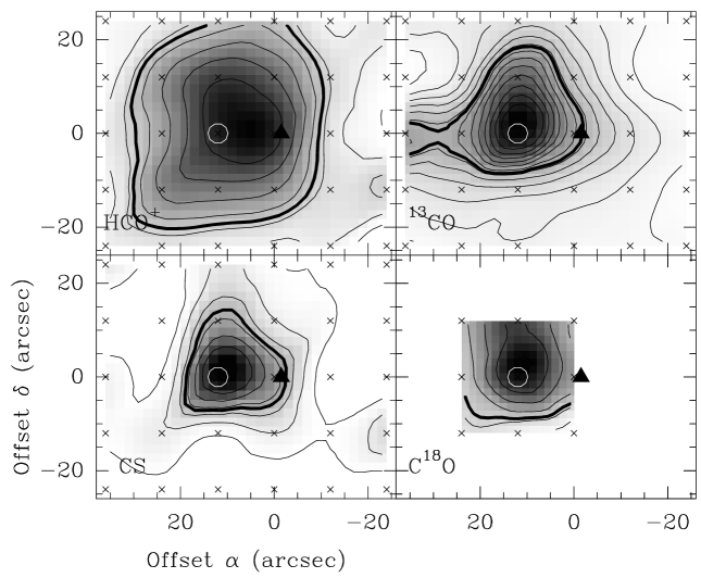
Figure 5: c Same as a, for Mol 59. Contour values (low(step)high, in Kkms^-1) are: 1(0.5)4.5 (HCO⁺); 6(4)62 (¹³CO); 1(1)7 (CS); 3(2)15 (C¹⁸O).

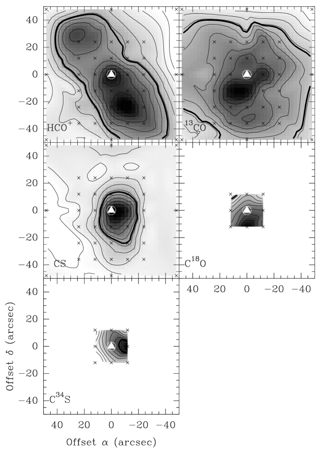
Figure 5: d Same as a, for Mol 75. Contour values (low(step)high, in Kkms^-1) are: 1(1)10 (HCO⁺); 15(6)81 (¹³CO); 1(2)19 (CS); 14(2)34 (C¹⁸O); 0.3(0.3)2.7 (C³⁴S).

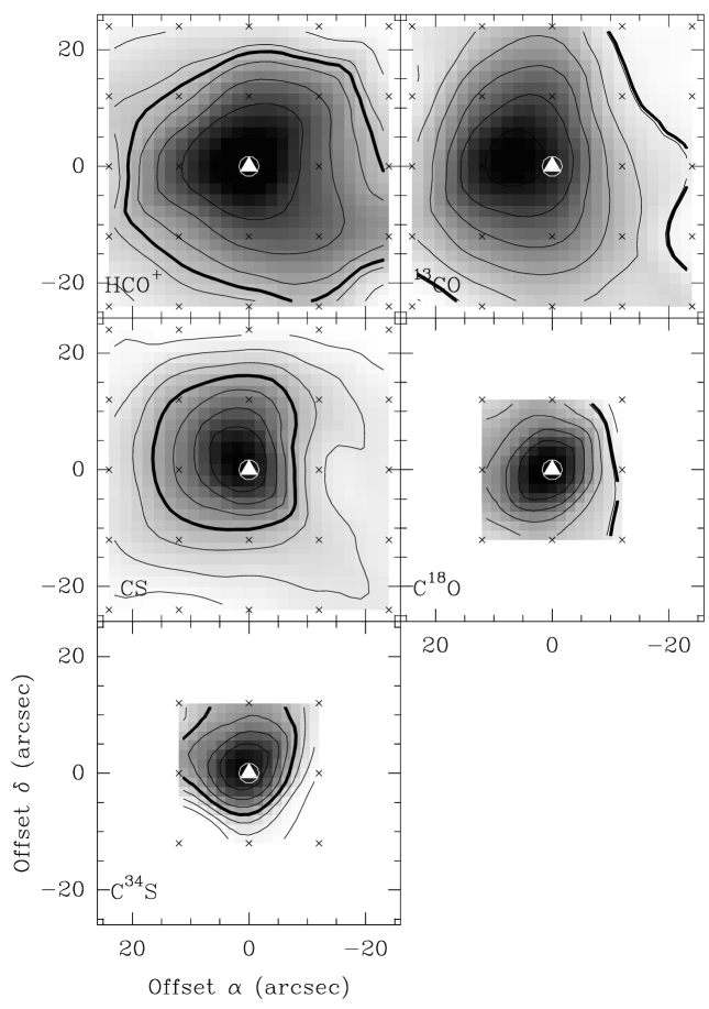
Figure 5: e Same as a, for Mol 77. Contour values (low(step)high, in Kkms^-1) are: 1(0.5)4 (HCO⁺); 18(4)42 (¹³CO); 1(1)8 (CS); 7(2)21 (C¹⁸O); 0.3(0.3)2.4 (C³⁴S).

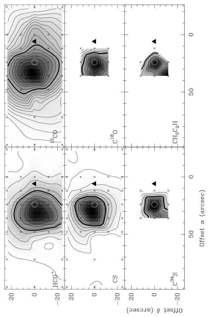
Figure 5: f Same as a, for Mol 98. Added here is a panel showing the distribution of the integrated emission over the K=0,1 components of CH₃C₂H(6$-$5). Contour values (low(step)high, in Kkms^-1) are: 1(2)17 (HCO⁺); 1(4)41(6)95 (¹³CO); 1(2)23 (CS); 3(3)35 (C¹⁸O); 0.5(0.5)4 (C³⁴S); 1(0.5)3.5 (CH₃C₂H).

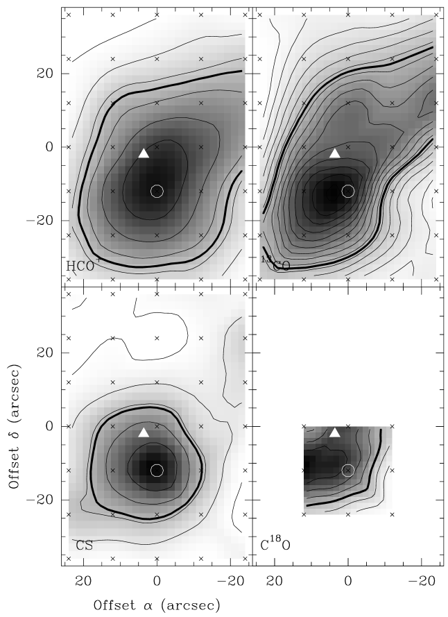
Figure 5: g Same as a, for Mol 117. Contour values (low(step)high, in Kkms^-1) are: 1(1)7 (HCO⁺); 5(4)70 (¹³CO); 0.5(1)5.5 (CS); 1(1)8 (C¹⁸O).

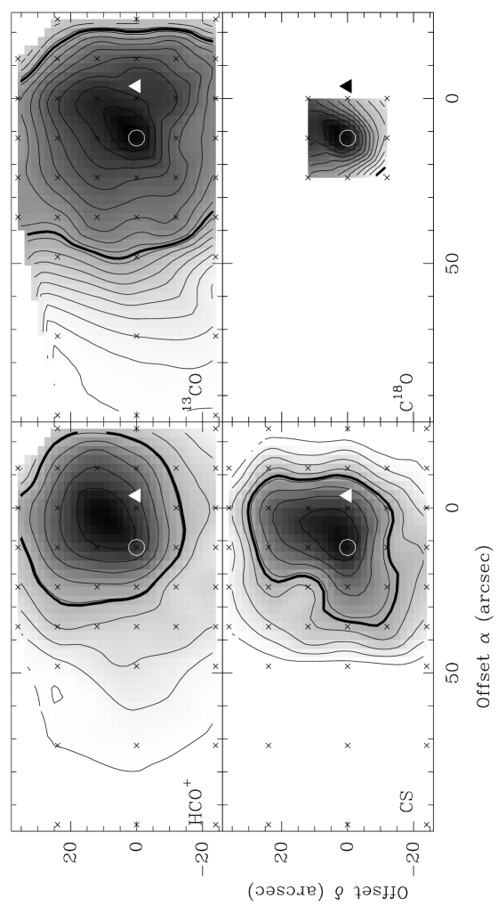
Figure 5: h Same as a, for Mol 118. Contour values (low(step)high, in Kkms^-1) are: 1(1)10 (HCO⁺); 1(4)71 (¹³CO); 0.5(1)8.5 (CS); 10(1)22 (C¹⁸O).

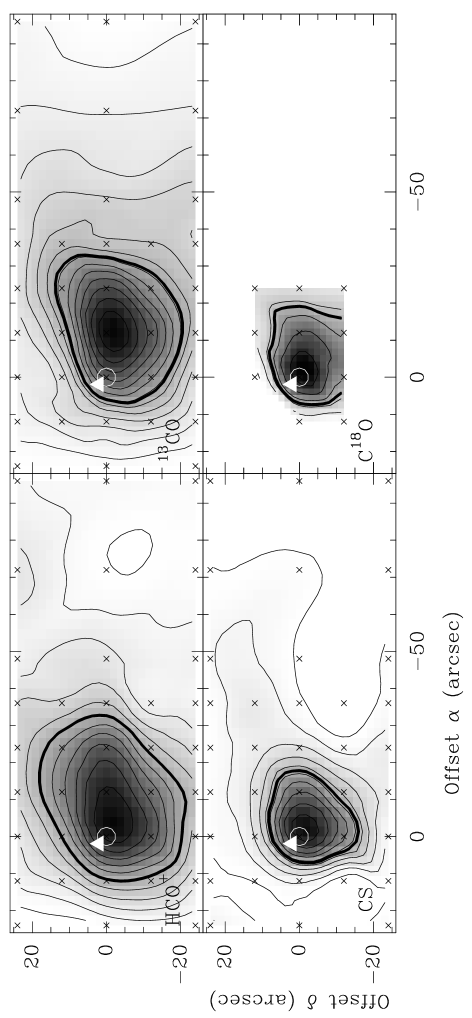
Figure 5: i Same as a, for Mol 136. Contour values (low(step)high, in Kkms^-1) are: 0.5(0.5)6 (HCO⁺); 1(4)57 (¹³CO); 0.5(1)10.5 (CS); 2(2)13 (C¹⁸O).

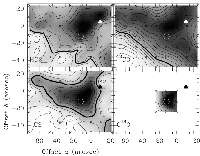
Figure 5: j Same as a, for Mol 155. Contour values (low(step)high, in Kkms^-1) are: 1.5(1)5.5 (HCO⁺); 8(4)72 (¹³CO); 0.5(1)6.5 (CS); 9(1)15 (C¹⁸O).

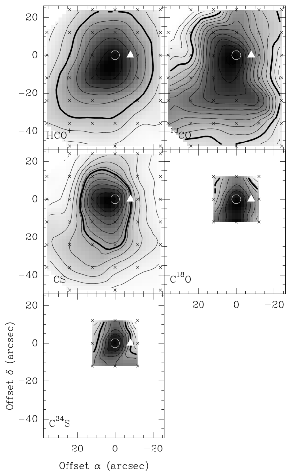
Figure 5: k Same as a, for Mol 160. Contour values (low(step)high, in Kkms^-1) are: 3(2)18 (HCO⁺); 31(6)110 (¹³CO); 0.5(2)22.5 (CS); 5(2)19 (C¹⁸O); 0.3(0.3)3 (C³⁴S).

The distributions of the integrated intensities of the emission of HCO⁺(1$-$0), ¹³CO(2$-$1), CS(3$-$2), C¹⁸O(2$-$1), C³⁴S(3$-$2) (where strong enough) and CH₃C₂H(6$-$5) (for Mol 98; the only source where it has been detected at more than one position) are shown in Figs. 5a$-$k. For easy reference we have shown in all maps the location of the IRAS source (not always coinciding with the map center), and the location of the peak position at which longer integrations were made. From these distributions we derived the (beam-corrected) source sizes, and a mass estimate of the molecular cores; the results are collected in Table 6. In this Table, column 1 gives the source name, column 2 the kinematic distance. In columns 3 to 6 we give the core size (in arcseconds and parsec), as determined from the transitions listed in the column headers. The sizes given here are those of the diameter of a circle with the same area as that enclosed by the FWHM contours in Figs. 5a$-$k. If the observed angular diameter is $\rm\theta_{obs}$, and the beam size at FWHP is $\rm\theta_{beam}$, then the beam-corrected size listed in the Table is $\rm\theta_{cor}=\sqrt{\theta_{obs}^{2}-\theta_{beam}^{2}}$. Finally, in column 7 we give a mass estimate of the core, as determined from the ¹³CO observations. We note that this mass represents all emission above the FWHM contour in Figs. 5a$-$k, regardless of whether all this emission is associated with the embedded YSO. For this latter information, and for the assumptions made in the mass estimate, we refer to Sect. 5. The mass estimates are lower limits, because only emission above the 50% level was used, and the FWHM contour is usually not closed inside the mapped area. The mass range is an order of magnitude, from 130 M_⊙ (Mol 118) to 2700 M_⊙ (Mol 3).

The FWHM contour of the ¹³CO emission extends beyond the limits of the maps in all but two of the observed sources. For the HCO⁺ emission we find the same, for most sources. Only the CS emission is well within the map boundaries, except for Mol 155, but even there the FWHM contour is almost closed inside the mapped region (Fig. 5j). Unfortunately the maps in C¹⁸O and C³⁴S are too small to allow a size determination.

Fig. 5 shows that the peak position of the higher-density tracers does not always coincide with that of the mm-continuum peak (= 0″,0″). However, for those sources for which new SCUBA observations (at 450 $\mu$m and/or 850 $\mu$m; Molinari et al., in preparation) are available, we find that the correspondence between molecular- and sub-mm-peak is good. The reason is that Molinari et al. (molinari00 (2000)) determined the location of the mm-peak from 5-point cross observations in most cases, rather than from mapping, which may have resulted in a not very accurate determination of the mm-peak in some cases. The IRAS source is usually within a few arcseconds from the mm-peak position, with the exception of Mols 3 (8.^′′7), 98 (5.^′′9), 155 (11.^′′9), and 160 (8″). Considering the sizes of the IRAS point source error ellipses (see e.g. Molinari et al. molinari00 (2000)), these deviations are not significant.

4.3 Line shapes

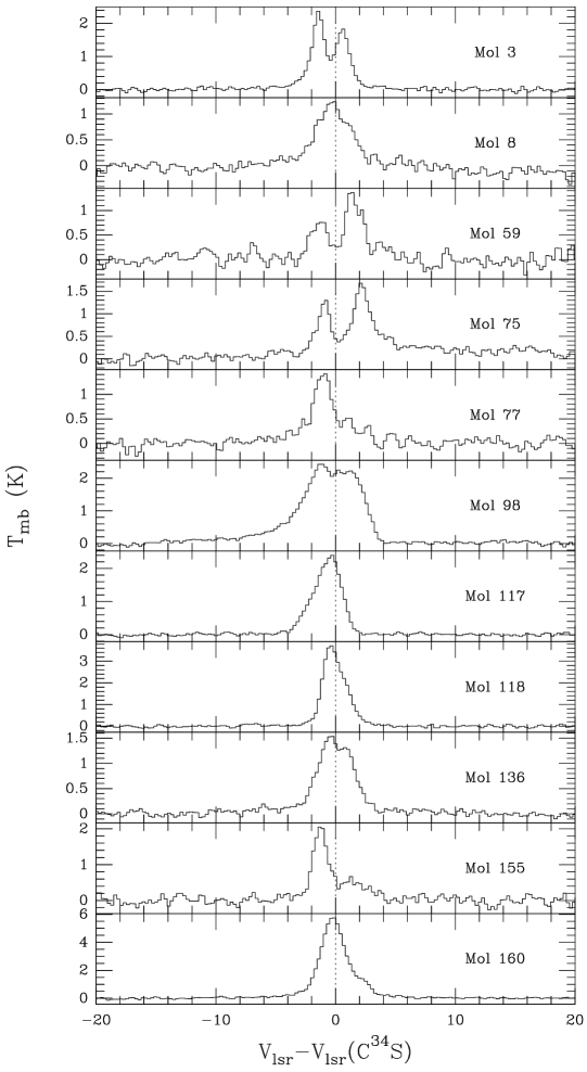
Figure 6: b As a, but for the HCO⁺(1$-$0) spectra

At many positions in the maps, but certainly at the peak positions, the signal-to-noise of the spectra is high enough for a detailed look at the line shapes. The rare isotopomer C³⁴S, with its low abundance and relatively high critical density, is a tracer of the denser regions of molecular clouds. Its line profiles can be fitted with a single Gaussian, with only a few exceptions: Mol 118 and Mol 160, where there are two components (see Sect. 5). In Mol 77 and 98, at low emission levels, there are deviations from a Gaussian on the blue side (perhaps due to outflowing gas). Because of this, the velocity of C³⁴S can be assumed to represent the velocity of the high-density gas, and can be used to identify asymmetries in the line profiles of the other transitions observed here. For this purpose, in Figs. 6a-d we show the spectra of ¹³CO(2$-$1), HCO⁺(1$-$0), CS(3$-$2), and C¹⁸O(2$-$1) aligned with the C³⁴S(3$-$2) velocity.

Fig. 6a shows that none of the ¹³CO profiles is a simple Gaussian, except perhaps for Mol 8, although broader emission is visible in the wings on both sides. Several of the profiles show dips, especially Mol 3, 59, and 77, while others (Mol 118, 155, 160) show shoulders. These deviations may be due to the superposition at that location of separate velocity components, or due to self-absorption. The latter can be produced either by an intervening colder cloud at the same velocity, or by a temperature gradient in the cloud itself. Profiles with stronger blue peaks can also be the signature of infalling gas (e.g. Myers et al. myers (2000)), although it is unlikely that such a phenomenon is visible in the present observations, considering the large distances of the sources in our sample, and the relatively large beam sizes involved.

The asymmetry of the profiles can be quantified by looking at the ratio of $\int Tdv$ on the blue- and red sides of the lines (where ‘blue’ and ‘red’ are relative to the C³⁴S velocity). The distribution of this ratio for each transition is shown in Fig. 7. The average ratio (indicated in each panel), is $>$1 for all tracers, indicating a clear blue asymmetry in the sample. The largest deviations from a Gaussian shape are found for the HCO⁺ profiles (Fig. 6b). By contrast, the CS spectra are all more or less symmetric with respect to the C³⁴S velocity: deviations from Gaussian profiles are seen in the CS spectra for Mol 3, 77, and 98, which are flat-topped, while there may be a dip in that for Mol 155. Mol 8, 59, 98, and 160 have ratios $\approx$1. The C¹⁸O profiles are also more Gaussian in shape than those of ¹³CO and HCO⁺, although less so than those of CS.

The interpretation of these numbers is not straightforward, because most spectra have multiple emission components (see sect. 5), some of which may not be associated with the embedded IRAS sources (about half of the objects under investigation are located in the inner Galaxy). Some general remarks can be made, however. The range in the ratios for the various tracers is an indication for their kinematical behaviour. For instance, the profiles of the tracers of the lower-density gas (like ¹³CO or C¹⁸O) show evidence of a kinematical behaviour different from that of the higher-density gas (as represented by the C³⁴S lines). On the other hand, the higher-density tracers (CS) tend to have narrower profiles, which are more symmetric with respect to the velocity of the high-density gas. The profiles of transitions like ¹³CO, which sample the more diffuse gas in which the high-density clumps are embedded, are shaped by larger-scale turbulence and by the superposition of various velocity components, that are not directly related to the molecular core in which the YSO is embedded. The HCO⁺ emission shows the largest average $\int Tdv$ blue/red ratio, as well as the largest range; this may be related to the fact that HCO⁺ is also produced in shocks, causing its kinematics to differ considerably from that of the C³⁴S gas.

The ratio of $\int Tdv$ CS/C³⁴S ranges between 4.7 (Mol 98) and 21.6 (Mol 117); the peak temperature ratio varies from 2.2 (Mol 77) to 15.4 (Mol 3). The ³²S/³⁴S-value for the local ISM $\approx$22 (Wilson & Rood wirood (1994)). The difference is likely due to CS being optically thick.

Note that if the Low objects are really representatives of a very early evolutionary stage of high-mass stars, they are expected to be associated with molecular outflows. These will contribute to the broadening of the line profiles discussed above, even though the presence of multiple emission components tends to obscure the visibility of line wings in the spectra.

4.4 Boltzmann plots

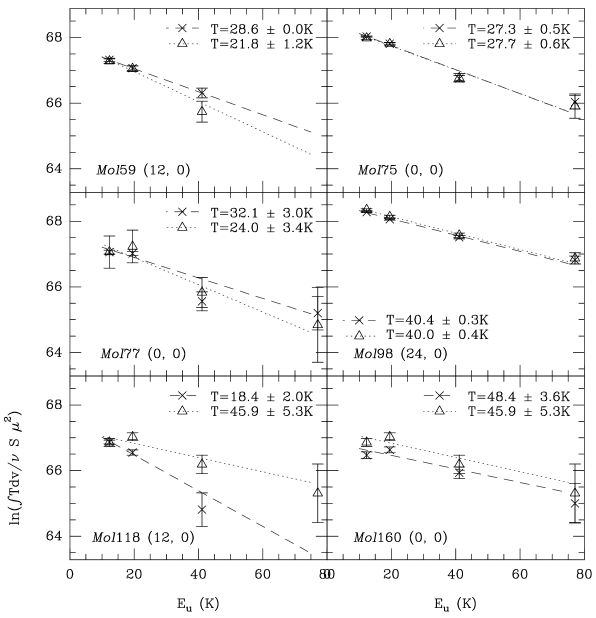
Figure 8: Boltzmann plots, constructed from the CH₃C₂H(6–5) observations. The results from the high- (0.23 kms^-1) and low-resolution (2.92 kms^-1) spectra are shown as crosses and triangles, respectively. The dashed and dotted lines are weighted least-squares fits through the data points. The sources are identified in the panels, where also the derived T_kin is given. Full results are presented in Table 7.

Fig. 8 shows the Boltzmann plots constructed from the CH₃C₂H(6–5) observations. From weighted least-squares fits to the data points, temperature and column densities can be derived (see e.g. Kuiper et al. kuiper (1984); Bergin et al bergin (1994)). The resulting rotational temperature T_rot, asumed to be equal to the gas kinetic temperature T_kin, and column densities, assuming optically thin emission, are collected in columns 4 and 6 of Table 7, respectively. The uncertainty in T_kin in column 5 is derived from that in the slope of the fit. An uncertainty for the column density N was obtained in two ways: by calculating an N_low and N_high with the extremes in T_kin, and taking the average difference between these two values and the N derived for T_kin (given in column 6); and by calculating the average difference in N as a result of the uncertainty in the slope of the fit. The uncertainties in N derived in these two ways were added in quadrature, and the resulting value is listed in column 7.

We list the parameters obtained from both the high- and the low-resolution spectra, for comparison. Only for Mol 118 is there a significant difference between the two. The derived T_kin are between 20 and 45 K, in agreement with the dust temperatures (Molinari et al. molinari00 (2000)). The low temperatures for these Low sources are in marked contrast with those found for members of the High group such as IRAS20126+4104 (Mol 119), where T${}_{\rm kin}\sim 200$ K (Cesaroni et al cesa97 (1997); from CH₃CN observations).

The CH₃CN(8–7) data for Mol 98 at (24″,0″) yield T${}_{\rm kin}\approx$666 K (425 K$-$1535 K) from the high-resolution spectrum, and 1073 K (577 K$-$7599 K) from the low-resolution spectrum. Though the uncertainties are very large, it does show that the temperature derived from CH₃CN is much larger than that, derived from CH₃C₂H, indicating that the emission of the former originates from deeper in the cloud, i.e. from closer to the embedded heating source (i.e. the YSO).

5 Comments on individual sources

In the following subsections we shall discuss the observed sources in some detail. If it helps our understanding of the molecular line data, we shall make use of as yet unpublished observations of ¹²CO(2–1) and C¹⁸O(2–1) [NRAO 12-m], 3.6-cm radio continuum [VLA D-array], and 450 $\mu$m and/or 850 $\mu$m [SCUBA]. We try to identify the velocity components of the molecular emission which are associated with the Molinari sources, and estimate the masses of these components from the ¹³CO data. The first step is to derive the column densities of the observed molecule, using the familiar equations (see e.g. Brand & Wouterloot bws151 (1998); Rohlfs & Wilson tools (1996)) with the appropriate constants for the molecule under consideration put in, and assuming the emission is optically thin. The excitation temperature T_ex is estimated from the NRAO CO spectra. To get the column density of H₂ we have used the relative abundance [H₂]/[¹³CO] = 5.0$\times 10^{5}$. Masses are estimated from the average H₂ column density, using all emission above the FWHM level of the integrated ¹³CO emission, and correcting the enclosed area for the beam of the observations. A correction for He ($\times 1.36$) has been applied as well. Mass estimates are lower limits, because not all emission is used, and the FWHM contour is not always closed within the area mapped with the 30-m. The results are collected in Table 8.

5.1 Mol~3

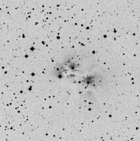
Figure 9: Optical image (Digital Sky Survey) of a 10′$\times$ 10′ region around Mol 3. N is up, E is left; the (0,0) position of the mapped region is indicated by the easternmost cross. The westernmost cross indicates the location of the 6-cm continuum peak detected by White & Gee white (1986) (GN0042.0$-$2; see text).

An optical image of a 10′$\times$10′ region around this object is shown in Fig. 9 (taken from the Digital Sky Survey: DSS). Clearly visible are several nebulous patches, that have been identified by Neckel & Staude (neckel84 (1984)), and which are known as GN0042.0$-$1 and GN0042.0$-$2 (Neckel & Vehrenberg neckel85 (1985)). In Fig. 9 the easternmost cross marks the position of the sub-mm peak (Molinari et al. molinari00 (2000)); the IRAS position is slightly to the NW of this, and almost coincides with the star which is located at the vertex of one of the nebulous patches. Neckel & Staude derive a photometric distance to this star (and to the star in the nebulosity to the SW) of 1.7 kpc, based on a B5 spectral type for both stars, and an assumed luminosity class V. White & Gee (white (1986)) observed both objects with the VLA D-array. GN0042.0$-$1 was not detected (at $>$0.3 mJy/beam), while GN0042.0$-$2 was detected at 6 cm. The westernmost cross in Fig. 9 indicates this radio continuum peak. The source has a peak flux density of 0.9 mJy/beam ($\int Fd\nu$=3.5 mJy); the spectral type derived from the radio data is B1-2, which is a large discrepancy with the Neckel & Staude optical data (B5). Hence, their photometric distance is uncertain, and we will use the kinematic distance.

GN0042.0$-$1, the collection of nebulosities nearest to Mol 3, was recently observed by Molinari et al. (in preparation) with the VLA D-array at 3.6 cm. They detected 3 faint radio sources, one of which (peak flux density $\approx$0.19 mJy/beam) is very close to the IRAS source. A second 3.6 cm source, with similar peak flux, lies at the same position as the H₂O maser and very close ($\sim$8″SE) to the 850 $\mu$m peak, both measured by Jenness et al. (jenness (1995)). This sub-mm peak lies $\sim$ $-$5″,$-$19″ from the sub-mm peak given in Molinari et al. (molinari00 (2000); taken as the 0,0 position of the present maps), who noted however that they missed the primary peak in their observations (a 5-point cross near the IRAS position only). Recent, unpublished SCUBA (850 $\mu$m) observations by Molinari et al. show that the true sub-mm peak coincides with the Jenness et al. 850 $\mu$m peak. In Fig. 5a it is seen that the CS peak is slightly offset to the SE with respect to the communal location of the other molecular peaks, the sub-mm peak, the H₂O maser, and one of the radio continuum sources.

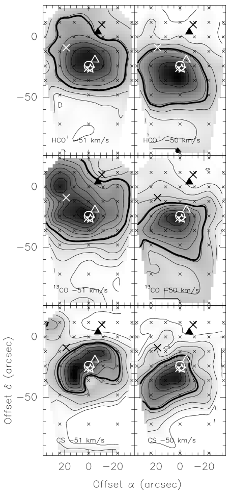
Figure 10:  Mol 3 data. Integrated emission of the red and blue emission (with respect to $-50.85$ kms^-1) for the indicated molecules. Red and blue integration limits are $-55,-48$ (HCO⁺), $-54,-48.5$ (¹³CO), and $-54,-48$ (CS). The symbols have the following meaning: filled triangle – IRAS source; open circle – molecular peak; open triangle – 850 $\mu$m peak; open star – H₂O maser position; big crosses – VLA-D array 3.6 cm peaks. Small crosses indicate the observed positions. Contour values are 0.3(0.5)3.9, 0.2(0.5)3.2 Kkms^-1 (HCO⁺ blue, red); 5.5(3)41.5, 2(3)31 Kkms^-1 (¹³CO blue, red); 0.2(0.4)3.2, 0.2(0.5)4.2 Kkms^-1 (CS blue, red); the thick contours indicate the FWHM level.

A look at Fig. 1a shows, that at the peak position in Mol 3 the ¹³CO, C¹⁸O, and HCO⁺ spectra are double-peaked, while the CS spectrum is flat-topped. The velocity of the (weak) C³⁴S line falls more or less in between the dip in the line profiles and the peak of the red component. Inspection of all profiles in the map, and of position-velocity plots of the molecular emission shows, that two components can be clearly seen over the whole mapped region; also the CS profiles are double-peaked away from the central position. In Fig. 10 we show the integrated areas over the blue- (at $-$50.85 kms^-1; left-hand panels) and the red side of the dip (right-hand panels). The sub-mm peak, the H₂O maser, and one of the 3.6 cm sources lie towards the peaks of the gas distribution for both components, although the correspondence with the blue peaks is slightly better (while the red component is more compact). In ¹³CO, blue component, a separate clump is visible, which may also be present in the HCO⁺ and CS maps.

5.2 Mol~8

The finding chart (at 8000 Å) published by Campbell et al. (campbell (1989)) shows that some very faint diffuse emission is associated with the IRAS source, which coincides with a star-like object. This source has been included in various studies. Ishii et al. (ishii (1998)) measured its NIR ($1.3-4.2\leavevmode\nobreak\ \mu$m) spectrum, and found the 3.1 $\mu$m absorption feature due to H₂O ice. This feature is found in environments protected from UV radiation, i.e. high-density molecular clouds, and is indeed often detected in deeply embedded YSOs (Ishii et al. ishii (1998)). Slysh et al. (slysh (1997)) found a strongly circularly polarized 2.7 Jy OH maser at 1665 MHz. No 6.7 GHz methanol maser was detected by MacLeod et al. (macleod (1998)), nor was this object detected by Harju et al. (harju (1998)) in their search for SiO maser emission.

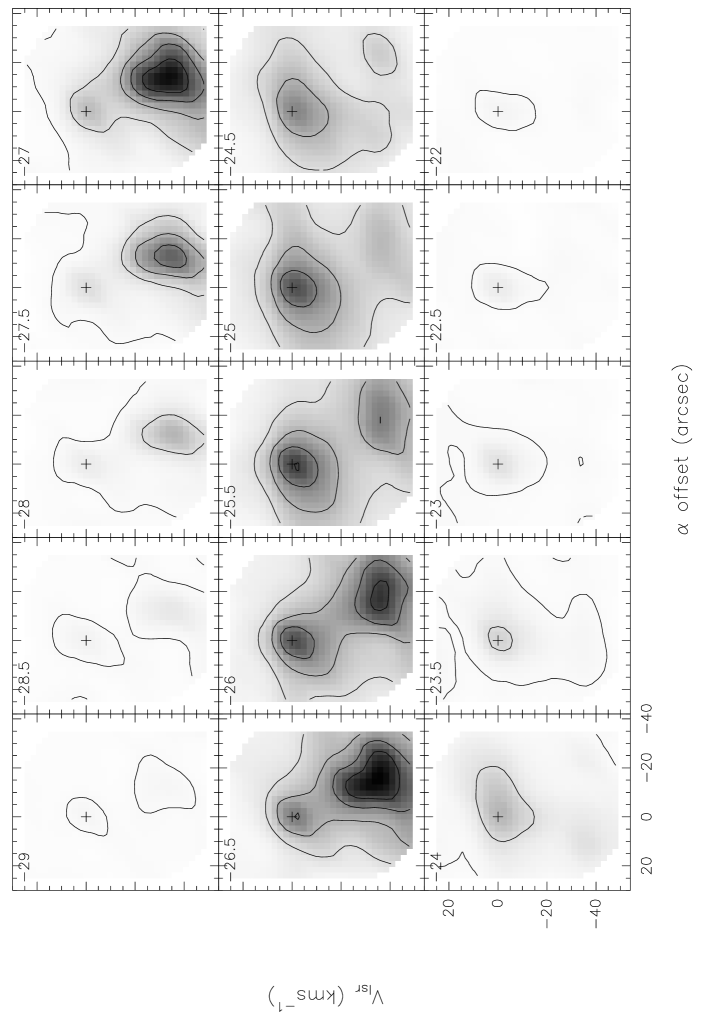
Figure 11: a Mol 8 data. Integrated emission of the ¹³CO line, shown in steps of 0.5 kms^-1. The cross indicates the position of the sub-mm peak ($\approx$ IRAS source position). Contours 0.5(4)17 Kkms^-1. The HCO⁺ and CS emission show the same behaviour, and are not shown

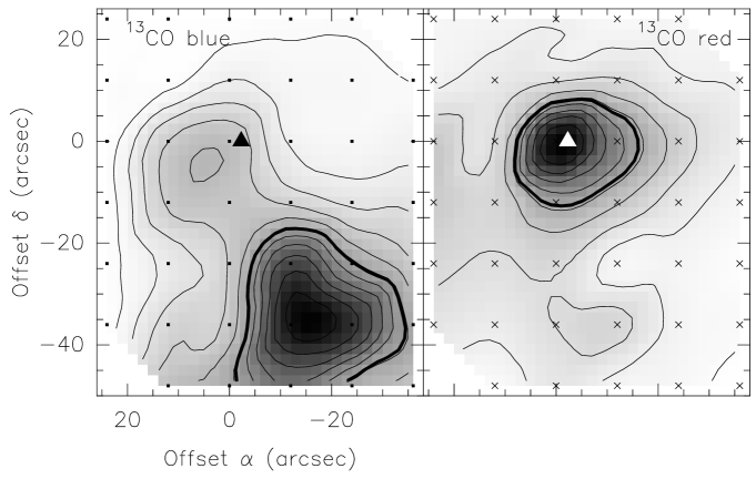
Figure 12: Mol 8 data. Emission under the ¹³CO lines, integrated over the blue and red components (separated by Gaussian fits). Contour values are 2(4)45 Kkms^-1 (blue) and 2(4)38 Kkms^-1 (red), respectively. The thick contours indicate the FWHM level. The triangle represents the IRAS position.

Although the spectra taken at the peak position (Fig. 1b) seem to show a single emission component, the channel maps in Fig. 11 clearly show the existence of two components, at $-$25.5 and $-$26.5 kms^-1 respectively. Although the velocity difference is small, the two components have a different spatial distribution and are therefore easily separated by Gaussian fitting to the line profiles. As an illustration we show in Fig. 12 the distributions of the areas under the blue and red components for ¹³CO. The redder (northern) component is associated with the embedded object.

Mol 8 is WB89 621 in the catalogue of Wouterloot & Brand (wb89 (1989)), who detected (with the IRAM 30-m) a strong CO(1$-$0) line at the IRAS position, and found evidence for wings. Wings are also visible in the present (¹³CO, HCO⁺, CS) spectra. Position-velocity plots show that wing emission occurs primarily in an area within 12″ from map center. The blue and red lobes are centered on the IRAS/sub-mm peak position; the closeness of the peaks of the lobes suggests that the bipolar flow is seen nearly pole-on.

5.3 Mol~59

The distance (5.7 kpc) to this object was based on V${}_{\rm lsr}[NH_{3}(1,1)]=93.7$ kms^-1. This line is however very weak (T${}_{\rm mb}=0.34\pm 0.09$ K), and the (2,2) line (0.23$\pm 0.10$ K) is found at V_lsr=97.7 kms^-1 (Molinari et al. molinari96 (1996)), casting some doubt on the validity of this distance calculation. The lines measured with the 30-m are however detected with reasonable signal-to-noise, and the emission is moreover clearly associated with Mol 59, as can be seen from Fig. 5c. The average velocity of $\approx$114.5 kms^-1, corresponds to d_kin=6.6 kpc (using the Brand & Blitz (brand (1993)) rotation curve).

This object lies in the galactic plane, $\sim$20° from the Galactic Center, and there is emission at various velocities. In the ¹³CO spectra we also found emission at 67 kms^-1 ($\sim$8 K) for instance. In the NRAO ¹²CO spectra, which have a larger velocity range, we find emission at practically all velocities between 0 and 170 kms^-1. In those spectra, emission is also found at $\sim$117-128 kms^-1; in the ¹³CO spectra (e.g. Fig. 1c) this is visible too, sometimes as a red shoulder to the line which has its peak at $\sim$115 kms^-1.

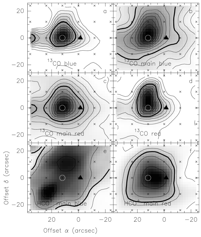
Figure 13: Mol 59 data. Emission in the ¹³CO (top 4 panels) and HCO⁺ (bottom 2 panels) lines, integrated over different velocity intervals: a: 105$-$111 kms^-1 [lowest contour 0.5, step 1 Kkms^-1]; b: 111$-$114.3 kms^-1 [5.5, 1.5 Kkms^-1]; c: 114.3$-$117 kms^-1 [1.5, 1.5 Kkms^-1]; d: 117$-$122 kms^-1 [0.5, 1 Kkms^-1]; e: 111$-$114.3 kms^-1 [0.5, 0.5 Kkms^-1]; f: 114.3$-$117 kms^-1 [0.5, 0.5 Kkms^-1]. Thick contours in each panel indicate the half-maximum level. The IRAS position is indicated by the triangle, the white circle is the position where longer integrations were made. Small crosses are the observed positions.

The spectra in Fig. 1c show a depression at 114.3 kms^-1, at least in HCO⁺, ¹³CO, and perhaps even in CS. The C³⁴S line, although weak, peaks more or less at the velocity of this depression, as the CH₃C₂H and C¹⁸O lines seem to do. All HCO⁺ and most ¹³CO spectra in the mapped region (30 spectra, covering an area of 60″$\times$48″) show this dip (the ¹³CO spectra at the edge of the map show asymmetries or shoulders), whereas CS has been detected at only a few positions near the peak at (12″,0″). This large area, and the relatively large beams involved in the observations, make self-absorption due to infalling gas an unlikely interpretation, also because there is little consistency between the relative strengths of the blue and red peaks in the profiles of the different tracers. The dip could be due to only a temperature gradient (without infall) in the cloud, or to an intervening colder cloud at the same velocity, but we prefer to interpret the spectra as being due to the superposition of several components, although this does not exclude the presence of self-absorption at the peak position. We integrated the emission over 5 velocity intervals, distinguishing between 5 components: $101-105(comp.\leavevmode\nobreak\ 1),105-111(comp.\leavevmode\nobreak\ 2),111-114.3(comp.\leavevmode\nobreak\ 3),114.3-117(comp.\leavevmode\nobreak\ 4)$, and $117-122(comp.\leavevmode\nobreak\ 5)$ kms^-1. The first component is present mostly in the E part of the map, and appears to have its maximum outside the mapped region. The distribution of the integrated ¹³CO emission from components (2) to (5) is shown in Fig. 13, together with that of components $(3)$ and $(4)$ for HCO⁺ (where the other components are much fainter or absent). Components $(3)$ and $(4)$ are dominating the spectra, and are referred to as the ‘main line blue’ and ‘main line red’, respectively. Component $(2)$ may be outflow emission connected to component $(3)$, while $(5)$ is most likely not outflowing gas, but emission from (a) separate component(s) (based on inspection of the 12-m ¹²CO spectrum). From Fig. 1c it is not evident which of the two main lines is associated with the sub-mm peak, but Fig. 13 suggests that it is the red component, which is more compact than the distribution of the blue line, and which has a maximum at the sub-mm peak in both ¹³CO and HCO⁺.

5.4 Mol~75

Ishii et al. (ishii (1998)) measured the NIR ($1.3-4.2\leavevmode\nobreak\ \mu$m) spectrum of this source, and found the 3.1 $\mu$m absorption feature due to H₂O ice. As for Mol 3, this is an indication of the presence of high-density material associated with this object. No 6.7 GHz methanol maser was detected by MacLeod et al. (macleod (1998)).

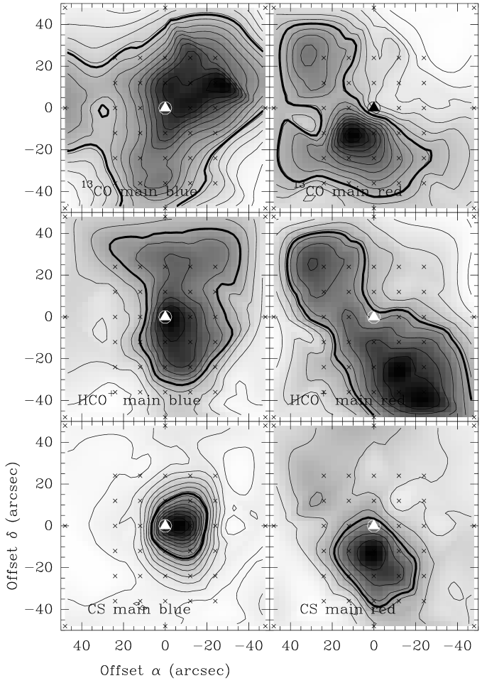
Figure 14: Mol 75 data. Emission in the ¹³CO (top 2 panels), HCO⁺ (middle 2 panels), and CS (bottom 2 panels) lines, integrated over the blue and red parts of the emission (see text). Thick contours in each panel indicate the half-maximum level. The IRAS position is indicated by the triangle, the white circle is the position where longer integrations were made. Small crosses are the observed positions. Contours: ¹³CO blue 8(2)37 Kkms^-1, red 4(2)36; HCO⁺ blue 0.2(0.2)2, red 0.2(0.8)7.4; CS blue 1(1)15, red 1(1)7.

Our observations show that the gas around the IRAS source is distributed over several clumps. This is particularly so in ¹³CO, where lines are found at V${}_{\rm lsr}\approx 41,49,53,56-58$ and $58-60$ kms^-1. The latter two components are also found in HCO⁺ and CS, suggesting that one or both of these are the associated components. We note that the NH₃(1,1) line is at 56.8 kms^-1, and that at the map’s peak position all lines (including CH₃C₂H) detected with the 30-m, except HCO⁺, have V${}_{\rm lsr}\approx 57$ kms^-1. The HCO⁺ line has a dominant component at $\sim$60 kms^-1, and the dip seen in Fig. 1d is at or close to the velocity where the other lines have their peak (except for CS, which peaks at the velocity of the blue component of the HCO⁺ emission). Note also that the KOSMA HCO⁺(4–3) spectrum seems to peak at the dip in the (1–0) spectrum (Fig. 2a), but Fig. 14 suggests the presence of two components.

We separated the two main components by integrating over the appropriate velocity intervals ($55-58.6-61.5,55-57.6-65$, and $54-58.2-62$ for ¹³CO, HCO⁺, and CS, respectively). The resulting distributions of the integrated emission are shown in Fig. 14. From this figure it is seen that the blue component peaks at or near the position of the IRAS source/850 $\mu$m peak, while the red component peaks south of that. Because the NH₃ and CH₃C₂H lines have the same velocity as the blue component, we assume that this defines the clump in which the FIR source is embedded.

We note that the HCO⁺ spectra in the central region of the map show a very broad red wing, up to V${}_{\rm lsr}\sim 80$ kms^-1 at (0″,0″) (i.e. more than 20 kms^-1 from the center of the red component; Fig. 1d). This broad emission is found in all the individual observations (ranging in number from 2 to 8) contributing to the average spectrum, and is therefore unlikely to be an artifact. This is strengthened by the fact that the wing is also present in the HCO⁺(4–3) spectrum (see Fig. 2). Some extended emision on the red side of the ¹³CO spectra is also present, although with a much smaller extent in velocity (up to 6 kms^-1 from the line center).

5.5 Mol~77

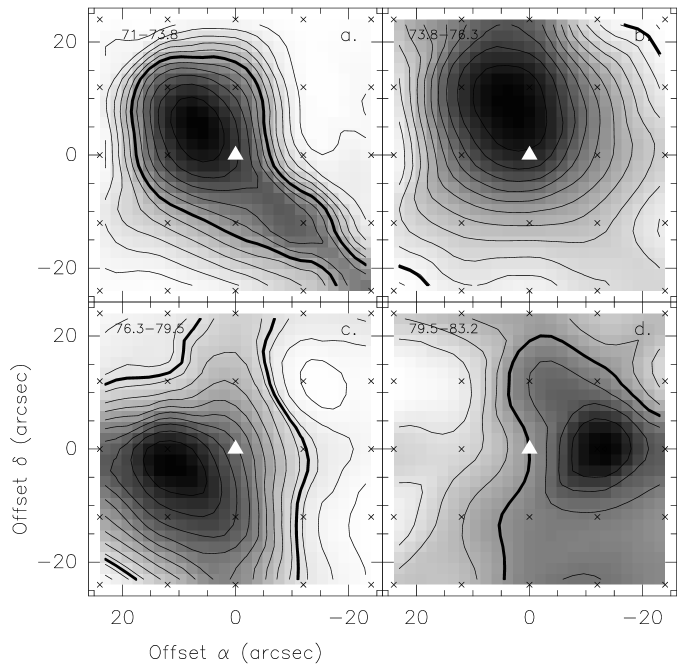
Figure 16: a. Distribution of $\int Tdv$ of the ¹³CO emission towards Mol 77, integrated over the velocity ranges indicated in the panels. In each panel an individual velocity component is isolated. Thick contours in each panel indicate the half-maximum level. The IRAS position is indicated by the triangle, and is identical to the position where longer integrations were made. Small crosses are the observed positions. Contours: 0.5(0.5)6 Kkms^-1 (panel a.); 10(1)22 (b.); 6(1)19 (c.); 0.5(0.5)4 (d.)

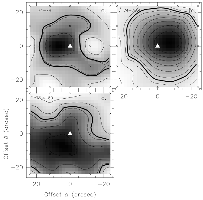
Figure 16: b. As a, but for HCO⁺. Contours: 0.2(0.2)0.8 Kkms^-1 (panel a.); 0.8(0.2)2.6 (b.); 0.2(0.2)1.2 (c.)

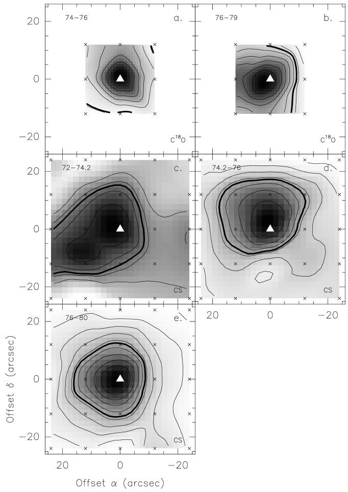
Figure 16: c. As a, but for C¹⁸O (panels a, b) and CS (panels c-e). Contours: 5(1)10 Kkms^-1 (panel a.); 3(1)11 (b.); 0.2(0.2)1 (c.); 0.2(0.4)3.4 (d.); 0.2(0.4)4 (e.)

The ¹³CO spectrum at (0″,0″) is double-peaked (Fig. 1e). All spectra of this molecule show either two peaks, or a shoulder (blue or red). The dip (or the start of the shoulder) is at the velocity of the C³⁴S line, which is also the velocity of the peak of the C¹⁸O and CH₃C₂H lines, and that of the NH₃(1,1) and (2,2) lines (Molinari et al. molinari96 (1996)). At all observed positions, the HCO⁺ spectrum shows only very weak emission on the red side of this dip. In Fig. 15 we compare the spectra of ¹³CO and HCO⁺ with the ¹²CO spectra we obtained with the NRAO 12-m (beam FWHP $\sim$29″). From this comparison it seems likely that the ¹³CO line profiles are the result of the superposition of two components, rather than being due to self-absorption. In the HCO⁺ spectra, the bluer component clearly is the dominant one. The ¹²CO spectra show broad emission at velocities $>$80 kms^-1, some of which is also seen in ¹³CO (see Fig. 16a), and is probably the result of additional emission components. On the blue side however (V${}_{\rm lsr}\lesssim 74$ kms^-1), the ¹²CO spectra are much steeper. At these velocities some emission is also present in the spectra of the molecules observed at IRAM (see Fig. 1e, and Fig. 16), and may be outflow emission associated with the component on the blue side of the dip; an eventual red component of this outflow is obscured by the emission of the other components redward of the dip.

To isolate the various components, we have integrated the line profiles over appropriately chosen velocity intervals; the results are shown in Fig. 16. From the dominance of the 75 kms^-1 component of HCO⁺, and the fact that it peaks at or very near the IRAS source and sub-mm peak, we conclude that the emission in the interval $\sim 74-76$ kms^-1 is likely to represent the associated component. However, also the emission between 76 and 80 kms^-1 peaks at that location, most clearly seen in the distribution for the density tracers C¹⁸O and CS (Fig. 16c), as does the emission between 71 and 74 kms^-1.

5.6 Mol~98

Towards this region we found an H₂O maser (Palla et al. palla91 (1991)), while a 6.7 GHz methanol maser was detected by MacLeod et al. (macleod (1998)). As they mention, methanol masers are unique indicators of massive star-forming regions, because unlike water- and hydroxyl masers, methanol masers have not been found towards stars of spectral type later than B2. These latter authors also detected circularly polarized 1665 MHz OH maser emission. Molinari et al. (1998a ) found no 2 and 6-cm radio continuum emission associated with this IRAS source. However, in recent VLA-D observations at 3.6-cm (Molinari et al., in preparation) continuum emission with a peak flux density $\sim$1 mJy/beam was detected at $\sim$(+10″,+14″) from the present map center. Recent SCUBA observations (Molinari et al., in preparation) at 450 $\mu$m show a sub-mm peak at $\sim$(+30″,+3″) from the present map center. We note that this is quite different from the offset of the sub-mm peak as given in Molinari et al. (molinari00 (2000)) ($-$10″,$-$10″ from the IRAS position, i.e. $-$4″,$-$10″ from the map center), which was however only based on a 5-point cross observation, and hence less trustworthy.

The present molecular observations show a quite compact core, even in ¹³CO, with a peak $\sim$25″ E of the IRAS source (Fig. 5f). The sum of all ¹³CO spectra of this source shows two absorption dips, at V${}_{\rm lsr}\sim 62$ kms^-1 and $\sim 70$ kms^-1, indicating that here the offset position ($\Delta\alpha,\Delta\delta=-1800$″,0″ from the center of the map) was not far enough from the molecular cloud in which the object is embedded. We have tried to correct for this by summing all ¹³CO spectra with narrow (V${}_{\rm lsr}\lesssim 60$ kms^-1) emission, fitting Gaussians to the dips (which have a strength of $\sim 1-1.5$ K), and adding those components to all ¹³CO spectra in the map. Unfortunately this does not correct for any absorption that might be present in the main line, but inspection of the spectra taken at positions without ¹³CO emission ($\Delta\alpha$= 96″) indicates that any such absorption will be $\lesssim$2.4 K ($\sim 2\sigma_{\rm rms}$ in the individual spectra at those positions).

The channel maps for this source indicate that there is only one emission component associated with the object (the ¹²CO spectra in the NRAO 12-m map, that covers an area of about 300″$\times$300″, show many emission components, but near Mol 98 the dominating one is that between $\sim 50-60$ kms^-1); the non-Gaussian profiles seen in Fig. 1f (flat top or shoulder) may be caused by saturation or self-absorption.

The spectra in Fig. 1f show non-Gaussian wings to all profiles, even that of C³⁴S. In Fig. 17 we show the distribution of the integrated emission over the line wings. Note that HCO⁺ has a relatively strong blue wing, which extends up to 15 kms^-1 from the velocity of the bulk of the molecular material. The outflow is bipolar in all 3 lines shown, and has the center of the line connecting the lobes at offset $\approx$(30″,5″), which puts it at the location of the 450 $\mu$m peak.

5.7 Mol~117

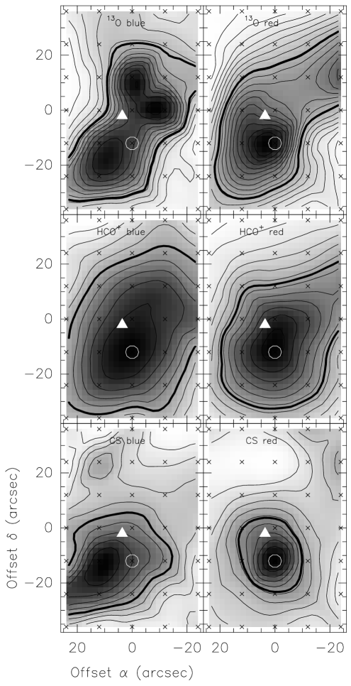
Figure 18: Mol 117 data. Emission in the ¹³CO (top 2 panels), HCO⁺ (middle 2 panels), and CS (bottom 2 panels) lines, integrated over the blue and red parts of the emission (see text). Thick contours in each panel indicate the half-maximum level. The IRAS position is indicated by the triangle, the white circle is the position where longer integrations were made. Small crosses are the observed positions. Contours: ¹³CO blue 3.5(1.5)23 Kkms^-1, red 4.5(2.5)49.5; HCO⁺ blue 0.2(0.2)2, red 0.2(0.4)4.8; CS blue 0.2(0.2)2, red 0.2(0.4)3.8.

On the DSS some faint diffuse emission is visible at the location of this object. Rather weak NH₃(1,1) emission was detected (Molinari et al. molinari96 (1996)) at V${}_{\rm lsr}\approx-36.4$ kms^-1, which is also the velocity at which HCO⁺(4–3) (see Fig. 2) is found. No 6.7 GHz methanol maser was detected by MacLeod et al. (macleod (1998)). The molecules observed at IRAM have their peak emission at V${}_{\rm lsr}\approx-35.7$ kms^-1 (Fig. 1g and Table 3). Our C¹⁸O(2–1) NRAO 12-m data show (at position 0″,0″, and with a 29″ beam) a double-peaked profile, with components at $-$37.9 and $-$35.9 kms^-1, and a dip at V${}_{\rm lsr}\approx-37$ kms^-1; the redder component therefore coincides with the velocities of the peak emission found at IRAM, while the NH₃ velocity lies closer to the dip in the NRAO C¹⁸O(2–1) spectrum. However, also the IRAM spectra show double-peaked profiles, as illustrated by the ¹³CO line at ($-$12″,0″) in Fig. 1g. In fact, at most positions we find that the line profiles have shoulders or double peaks, with the dip always at the same velocity. We therefore analyze the data in terms of the superposition of two emission components. The components are separated by integrating between $-$40 and $-$36.9 kms^-1 (blue) and $-$36.9 and $-$33 kms^-1 (red) for ¹³CO and HCO⁺, and $-$39.5 and $-$36.3 kms^-1 (blue) and $-$36.3 and $-$33 kms^-1 (red) for CS. The distributions of the integrated emission are shown in Fig. 18. Because the red peak seems to be the dominant one, we assume this is the associated component.

5.8 Mol~118

This is the object with the smallest kinematical distance (1.6 kpc) in the sample. The (0,0) position of the maps, and the IRAS source (at offset $-$3.^′′7,0″) are located in a dark cloud, which is surrounded by diffuse emission. No 6.7 GHz methanol maser was detected by MacLeod et al. (macleod (1998)).

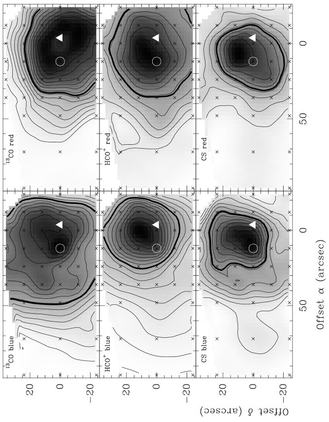
Figure 19: Mol 118 data. Emission in the ¹³CO (top 2 panels), HCO⁺ (middle 2 panels), and CS (bottom 2 panels) lines, integrated over the blue and red parts of the emission (see text). Thick contours in each panel indicate the half-maximum level. The IRAS position is indicated by the triangle, the white circle is the position where longer integrations were made. Small crosses are the observed positions. Contours: ¹³CO blue 2(3)45 Kkms^-1, red 1(1)15; HCO⁺ blue 0.2(0.4)6.8, red 0.2(0.2)2; CS blue 0.2(0.4)4.6, red 0.2(0.4)3.4.

The spectra shown in Fig. 1h are non-Gaussian, and as evidenced by the C³⁴S spectrum, and the superimposed ¹³CO and C¹⁸O spectra at offset (12″, 12″), this is due to the presence of two velocity components. In addition, emission in the wings of the profiles is visible, which may be due to outflow, or to additional components. These wings are also visible in the NRAO CO(2–1) spectra. We separate the two main (‘blue’ and ‘red’) components by integrating over the following velocity intervals: 6.5–8.5–9.4 kms^-1 (¹³CO); 6.5–8.4–9.4 kms^-1 (HCO⁺); 6.8–8.2–9.2 kms^-1 (CS). These integration limits omit the wing emission. The distribution of the emission in each component is shown in Fig. 19. The NH₃ velocity is 7.8 kms^-1, that of CH₃C₂H is 7.9, and thus coinciding with the (more intense) blue component, which we will take as the associated one.

5.9 Mol~136

Inspection of the data reveal that there is only one emission component detected towards this source. The line profiles are non-Gaussian, being skewed towards the blue (see Fig. 1i). This is also seen in the ¹²CO(1–0) line profile (Wouterloot & Brand wb89 (1989); source WB89 93). Low-level emission is also seen extending over a few kms^-1 from the central line velocity; the distribution of the integrated emission in these wings is shown in Fig. 20. The blue emission peaks near the IRAS source position (which is also the peak of the sub-mm emission), while the red component has its maximum more to the West.

Although Molinari et al. (1998a ) did not detect associated radio continuum emission (VLA, 2 and 6-cm), deeper observations at 3.6-cm with the VLA D-array by Molinari et al. (in preparation), reveal diffuse emission (peak flux density $\sim$6.2 mJy/beam) just NE of the IRAS source.

5.10 Mol~155

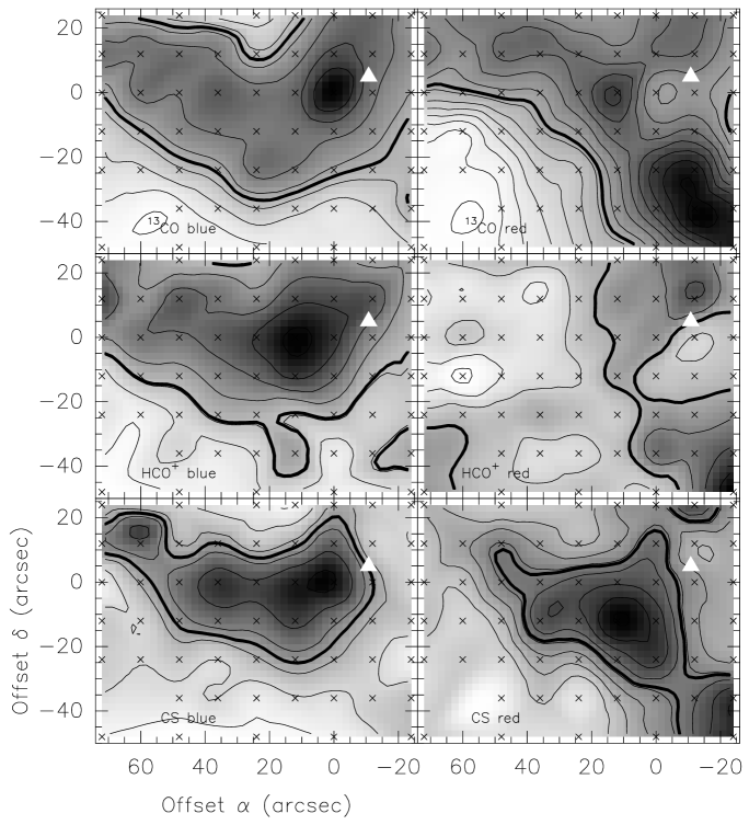
Figure 21: Mol 155 data. Emission in the ¹³CO (top 2 panels), HCO⁺ (middle 2 panels), and CS (bottom 2 panels) lines, integrated over the blue and red parts of the emission (see text). Thick contours in each panel indicate the half-maximum level. The IRAS position is indicated by the triangle. Small crosses are the observed positions. Contours: ¹³CO blue 5(5)45 Kkms^-1, red 3(3)44; HCO⁺ blue 0.5(0.5)4, red 0.2(0.4)3; CS blue 0.2(0.8)4.4, red 0.2(0.4)3.4.

The emission of especially ¹³CO and HCO⁺ is quite extended in this source (see Fig. 5j). The line profiles are similar to those in Mol 77 (cf. Figs. 1e and j): The profiles of ¹³CO and HCO⁺ show a dip or a shoulder everywhere, while for the latter molecule the blue component is much stronger than the red one at every observed position. The dip or shoulder is at V${}_{\rm lsr}\sim-51.1,-50.7$ and $-51.0$ kms^-1 for ¹³CO, HCO⁺,and CS, respectively. The velocity of the NH₃(1,1) line is at $-$51.5 kms^-1, thus in the velocity range of the blue component. We separate the two emission components by integrating blue- and redwards of the dip. The resulting distributions of the integrated emission are shown in Fig. 21. The dominance of the HCO⁺ blue component is clearly visible there. We note that towards this source observations of SiO(2–1) (Harju et al. harju (1998)) have yielded no detections.

5.11 Mol~160

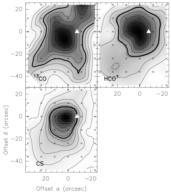
Figure 22: Mol 160 data. Area under the main component (subtracting components using Gaussian fits), for the molecules marked in the panels. The triangle indicates the IRAS position. Contour values are 7(6)61 Kkms^-1 (¹³CO); 1(2)14 Kkms^-1 (HCO⁺); 1(2)19 Kkms^-1 (CS). The thick contours mark the FWHM values.

This source has been observed and discussed extensively by Molinari et al. (1998b ), who concluded that this is a very good candidate massive Class 0 object. Inspection of the line profiles at the peak position (Fig. 1k; especially C¹⁸O) strongly suggests the presence of two velocity components. Individual ¹³CO spectra indicate that there might be more than two components; we also note that the dip, or shoulder, in these spectra is not always at the same velocity. This may be an indication of the presence of a velocity gradient in the ¹³CO emission, and separating the contribution of the various components by integrating over fixed velocity intervals is hazardous. We have therefore performed Gaussian fits to the profiles of ¹³CO, HCO⁺, and CS (even though for the latter two we do not see a shift in the position of the dip (if at all) with position). Based on the V_lsr of the NH₃(1,1) and CH₃C₂H(6–5) lines ($-50.0$ and $-50.45$ kms^-1 respectively), we identify the main emission component. After subtraction of the other Gaussian components, we integrated the spectra; the resulting distributions of the emission are shown in Fig. 22. The emission peaks lie close to the 3.4-mm continuum peak found with OVRO by Molinari et al. (1998b ).

Fig. 23 shows a series of Right Ascension versus V_lsr plots for the ¹³CO line, at the Declination offsets labeled in each panel. Especially at positive Declination offsets the distribution of the emission is suggestive of a velocity gradient, with velocity increasing (becoming redder) from E to W. The gradient is of the order of 1.4 kms^-1pc^-1. The HCO⁺ data for the main component indicate a gradient of $\sim$0.8 kms^-1pc^-1; no clear velocity gradient is present in the CS data.

The line profiles in Fig. 1k show some low-level emission in the wings. For HCO⁺ and CS we show the integrated wing emission in Fig. 24. As was found on a much smaller scale in our OVRO observations of HCO⁺ and SiO (Molinari et al. 1998b ), the blue and red lobes almost overlap, and we are seeing the outflow nearly pole-on.

Finally we note that, although Molinari et al. (1998a ) found no radio continuum emission (at 2 and 6-cm) towards this object, there is an 11-cm radio continuum source (F3R 3484; integrated flux density 0.16 Jy, peak flux density 130 mJy) at this location (Fürst et al. fuerst (1990)). Deep VLA-D array observations at 3.6-cm (Molinari et al., in preparation) reveal a double-lobed emission structure. The extent of the lobes (at a level of $\sim$5% of the peak value) is $\sim$93″$\times$127″ for the W lobe ($\int Fd\nu\approx$60 mJy), and $\sim$50″ for the E lobe $\int Fd\nu\approx$17 mJy). The 3.4-mm continuum source (Molinari et al. 1998b ) lies at the sharp E edge of the larger, westernmost radio lobe, at $\sim 21$″ to the NE from its peak. The general location of the radio lobes coincides with the diffuse emission seen in the 15$\mu$m ISOCAM map (see Molinari et al. 1998b ), although the extent of the radio continuum emission is larger. It is unclear whether this radio emission is associated with the embedded object.

6 Discussion and conclusions

The most direct result of this work is that all of the observed sources are clearly associated with well-defined molecular clumps. It must be stressed that such clumps are seen in various molecular tracers and are hence real physical entities. The main goal of our observations was to obtain a picture of the molecular environment associated with Low sources and look for any evidence supporting the hypothesis that Low sources are the precursors of High sources. In this scenario, the former correspond to YSOs still accreting mass from the surrounding environment, whereas the latter are ZAMS early type stars still deeply embedded in their natal cores. The most direct way to verify this is to make high-angular resolution observations of the Low objects to study their structure and physical parameters, and indeed we are already performing this type of investigation on a limited number of objects selected on the basis of the present study. However, it is also possible to draw some tentative conclusions by comparing our sample with a sample of High sources studied by Cesaroni et al. (cesa99 (1999)) with the same telescope and in the same lines. For this purpose, we have collected in Table 9 all the parameters derived from both studies: for each quantity we give the minimum, maximum, and mean values. We note that sources Sh-2 233 and NGC 2024 from the Cesaroni et al. (cesa99 (1999)) sample have not been considered here, as they satisfy neither the requirements of the High-, nor of the Low sources.

In Table 9, $\Theta$ is the angular diameter of the clumps after deconvolution of the beam, $D$ is the corresponding linear diameter, T_mb(K) and T_b(K) are the main beam and intrinsic (after correcting for the beam filling factor) brightness temperatures, FWZI the line full width at zero intensity, FWHM the line full width at half maximum, M_vir the virial mass, and M_CD the mass obtained by integrating the line emission over the line profile and over the whole emitting region. For the latter estimate we have assumed LTE at 30 K and abundances of $1.1\times 10^{-6}$, $10^{-9}$, $10^{-8}$, $4.5\times 10^{-10}$ respectively for ¹³CO, HCO⁺, CS, and C³⁴S (Irvine et al. irvine (1987)). Note that the ¹³CO abundance is what was used by Cesaroni et al. (cesa99 (1999)), and is slightly smaller (by a factor of 1.8) than what we used in Sect. 5. In only four Low sources (Mol 8, 77, 98, and 160) the C³⁴S(3–2) emission was strong enough to be mapped; sizes, masses, and intrinsic brightness temperature derived from this molecule, reported in Table 9 are derived from these four objects only, and may not be representative.

Inspection of Table 9 reveals a few interesting differences between the two samples in spite of the similar bolometric luminosities. Relative to the clumps associated with High sources, those around the Low sources are more massive (2–4 times; except for C³⁴S), larger ($\sim$3 times), less bright (1–3 times), have smaller line widths ($\ga$1.5 times). The Low sources also appear to be less dynamically stable than the High sources since they typically have a smaller ratio $\rm M_{vir}/M_{CD}$, which is a measure of the balance between gravitation and turbulence: the smaller it is, the weaker is the support against collapse. The results are therefore consistent with Low sources representing an evolutionary phase prior to that of High sources. In fact, the larger diameters of the Low clumps suggest that they should still undergo substantial contraction, as indicated by the lower densities. Moreover, the lower brightness temperatures may be considered an indication of lower temperatures and/or optical depths, both expected in an early phase of the evolution. Finally, the broader lines in the High sample might be related to the existence of a larger number of molecular outflows and hence of YSOs already formed: such outflows could support the surrounding clump from collapse by injecting high velocity gas, thus accounting for the higher ratio $\rm M_{vir}/M_{CD}$.

We note that the clump mass as reported in Table 8 increases with the L_fir of the IRAS source (see Fig. 25a; a least-squares fit to mass versus luminosity gives a slope of $\sim 1.17\pm 0.22$ and a corr. coeff. of $\sim$0.57). Then, assuming that each clump contains a single protostellar object, we can obtain an estimate of the mass of the central object from the known value of L_fir. Using the models of Palla & Stahler (palsta (1992)) for an accretion rate of $10^{-4}$ M_⊙ /year, we compute the mass of a protostar that produces a luminosity, L_proto, equal to the observed L_fir. Note that L_proto includes a component from accretion and one due to gravitational contraction. For the range of luminosities considered here, the latter term dominates. The resulting protostellar masses are plotted against clump masses in Fig. 25b. The highest mass that the models of Palla & Stahler (palsta (1992)) can give is $\sim$17 M_⊙, hence the two lower limits for two of the objects (Mol 3 and 8). The lowest protostellar mass is for Mol 118 and amounts to 7.4 M_⊙. From Fig. 25b we see that there is a weak dependence on clump mass. A fit to the data points shows that $\rm M_{proto}\propto M_{clump}^{0.30\pm 0.07}$. Note that the slope of this relation is similar to that found by Larson (larson (1982)) in his study of young stars and molecular clouds, who found that the maximum mass of stars is related to the mass of the cloud as $\rm M_{star}\propto M_{cloud}^{0.43}$.

In conclusion, we believe that our results lend support to the evolutionary scenario previously proposed by us (Palla et al. palla91 (1991); Molinari et al. molinari96 (1996); Molinari et al. 1998a ), according to which the majority of Low sources will eventually evolve into High sources.

Table 1: Observed transitions

Molecule	Frequency	Vres1	HPBW	Notes
	(MHz)	(kms-1)	(″)
IRAM 30-m
HCO+(1$-$0)	89188.518	0.26	27	a
13CH3CN(5$-$4)	89331.297	3.36	27	a,b
CH3C2H(6$-$5)	102547.984	0.22	23	b
C${}^{34}{\rm S}$(3$-$2)	144617.147	0.16	17	c
CH3OH(Vt=1)	145103.230	2.07	17	c
CS(3$-$2)	146969.049	0.16	16	d
CH3CN(8$-$7)	147174.592	2.04	16	b,d
C${}^{18}{\rm O}$(2$-$1)	219560.328	0.11	11
13CO(2$-$1)	220398.686	0.11	11	e
CH3CN(12$-$11)	220747.268	1.36	11	b,e
KOSMA 3-m
HCO+(4$-$3)	356734.253	0.14	74
1 Highest velocity resolution available
a,c,d,e Transitions measured in same receiver
b Frequency of the K=0 transition

Table 2: Observed Sources

(1)	(2)	(3)	(4)	(5)	(6)	(7)	(8)	(9)	(10)	(11)	(12)
Mol	$\alpha$(1950)♠	$\delta$(1950)♠	$\it{l}$	$\it{b}$	IRAS	Vlsr(NH3)	dkin	Lfir	H2O	Radio1	mm2
#	(h m s)	(° ′ ″)	(°)	(°)		(kms-1)	(kpc)	(104 L⊙)
♣3	00 42 06.3	+55 30 50	122.015	$-$7.072	00420+5530	$-$51.2	7.7	5.15	Y	N3	Npp
8	05 13 46.0	+39 19 10	168.061	+0.821	05137+3919	$-$25.4	10.8	3.935	Y	N3	Y
59	18 27 49.7	$-$10 09 19	21.561	$-$0.030	18278$-$1009	+93.7	†6.6	1.465,6	Y	N	Y
♣75	18 51 06.4	+01 46 40	34.821	+0.351	18511+0146	+56.8	3.9	1.305	N	U	Y
77	18 52 46.2	+03 01 13	36.115	+0.554	18527+0301	+76.0	5.3	0.905	N	N	Y
98	19 09 13.0	+08 41 27	43.035	$-$0.447	19092+0841	+58.0	4.5	0.925	Y	U3	Y
♣117	20 09 54.3	+36 40 37	74.161	+1.644	20099+3640	$-$36.4	8.7	2.515	N	Y	Y
♣118	20 10 38.3	+35 45 42	73.479	+1.016	20106+3545	+7.8	1.6	0.18	N	N	Npp
136	21 30 47.1	+50 49 01	94.262	$-$0.411	21307+5049	$-$46.7	6.2	1.165	Y	U3	Y
♣155	23 14 03.4	+61 21 17	111.871	+0.820	23140+6121	$-$51.5	5.2	1.065	N4	Y	Y
♣160	23 38 31.2	+60 53 43	114.531	$-$0.543	23385+6053	$-$50.0	4.9	1.605	Y	N	Y
♠ map center (sub-mm peak Molinari et al. molinari00 (2000))
♣ peak position also observed in HCO+(4$-$3); see Sect. 3
† Derived from the present data; see Sect. 5
1 U = unassociated radio source is within 3′ radius
2 Compact mm-emission; Npp = Detected, but missed primary peak; see Molinari et al. (molinari00 (2000))
3 Recently detected with the VLA-D array at 3.6-cm (see Molinari et al. molinari00 (2000)); detected signal is compatible with the
${}^{\ }$ non-detections at 2 and 6-cm reported in Molinari et al. (1998a )
4 Maser discovered by Valdettaro et al. (u2 (2000))
5 Luminosity from Molinari et al. (molinari00 (2000))
6 Corrected for revised distance

Table 3: Line parameters at peak position

Line	Vres	rms	Vmin	Vmax	Tmb	Vlsr	$\Delta v$	$\int$Tmbdv1	$\int$Tmbdv2
	(kms-1)	(K)	(kms-1)	(kms-1)	(K)	(kms-1)	(kms-1)	(Kkms-1)	(Kkms-1)
Mol 3 (0″,$-$24″)
HCO+(1$-$0)	0.26	0.045	$-$53.8	$-$48.3	2.4	$-$51.9	1.3	6.2	6.6
							3.2
13CO(2$-$1)	0.11	0.78	$-$53.2	$-$48.4	27.0	$-$52.0	1.5	67.3	68.8
							3.13
CS(3$-$2)	0.16	0.12	$-$53.2	$-$48.5	2.1	$-$50.8	2.7	5.7	5.8
C18O(2$-$1)	0.11	0.16	$-$52.8	$-$49.0	6.7	$-$50.3	2.7	16.6	16.9
C34S(3$-$2)	0.16	0.073
smoothed:	0.65	0.039	$-$52.0	$-$49.4	0.1	$-$50.4	2.6	0.3	0.4
Mol 8 (0″,0″)
HCO+(1$-$0)	0.26	0.082	$-$30.7	$-$21.5	1.3	$-$25.3	3.4	5.3	6.4
13CO(2$-$1)	0.11	0.25	$-$29.6	$-$20.3	16.6	$-$25.4	2.8	56.6	59.4
CS(3$-$2)	0.16	0.16	$-$27.8	$-$22.7	4.1	$-$25.1	2.1	10.3	10.5
C18O(2$-$1)	0.11	0.14	$-$27.3	$-$22.6	3.5	$-$25.3	2.1	7.7	7.9
C34S(3$-$2)	0.16	0.079	$-$26.3	$-$23.9	1.2	$-$25.1	1.3	1.7	2.0
Mol 59 (12″,0″)
HCO+(1$-$0)	0.26	0.11	111.8	118.9	1.4	115.5	1.8	4.1	4.2
							4.23
13CO(2$-$1)	0.11	0.49	107.2	120.1	9.1	115.1	5.5	58.3	61.3
CS(3$-$2)	0.16	0.32	112.3	115.8	2.4	114.8	2.9	5.4	6.8
C18O(2$-$1)	0.11	0.25	111.0	117.1	4.9	113.4	2.0	13.3	15.8
C34S(3$-$2)	0.16	0.12	113.6	115.1	0.4	113.9	1.9	0.5	0.8
Mol 75 (0″,0″)
HCO+(1$-$0)	0.26	0.069	54.7	69.1	1.6	59.6	1.8	7.4	9.8
							2.93
13CO(2$-$1)	0.11	0.55	50.5	61.3	11.5	57.0	4.4	59.2	65.3
CS(3$-$2)	0.16	0.20	53.6	61.2	5.0	56.8	2.9	17.7	17.8
C18O(2$-$1)	0.11	0.17	53.0	60.4	8.1	57.3	3.3	27.9	28.3
C34S(3$-$2)	0.16	0.094	56.2	59.3	0.7	57.0	1.9	1.4	1.6
Mol 77 (0″,0″)
HCO+(1$-$0)	0.26	0.090	72.1	79.1	1.4	75.2	1.8	4.0	4.3
13CO(2$-$1)	0.11	0.35	71.9	82.1	10.1	75.1	4.2	42.5	42.9
CS(3$-$2)	0.16	0.25	72.8	78.0	2.6	75.5	2.9	7.4	7.8
C18O(2$-$1)	0.11	0.22	73.8	78.3	8.5	75.7	2.4	20.8	21.1
C34S(3$-$2)	0.16	0.073	74.1	77.5	1.0	76.4	1.6	1.9	2.4
1 Integral taken between Vmin and Vmax
2 Integral taken between velocities where Tmb=0 K
3 In line profiles with a ‘dip’ which is $<$ 0.5Tpeak, the $\Delta v$ on the second line is the FWHM taken over
${}^{\ }$ the whole line

Table 3: (continued)

Line	Vres	rms	Vmin	Vmax	Tmb	Vlsr	$\Delta v$	$\int$Tmbdv1	$\int$Tmbdv2
	(kms-1)	(K)	(kms-1)	(kms-1)	(K)	(kms-1)	(kms-1)	(Kkms-1)	(Kkms-1)
Mol 98 (24″,0″)
HCO+(1$-$0)	0.26	0.041	45.1	61.4	2.4	56.4	5.7	14.8	15.0
13CO(2$-$1)	0.11	0.22	53.0	63.2	17.7	57.0	4.0	74.6	75.1
CS(3$-$2)	0.16	0.096	52.2	63.8	3.1	56.9	6.1	18.9	20.2
C18O(2$-$1)	0.11	0.13	53.7	62.3	9.0	58.3	3.6	33.7	33.9
C34S(3$-$2)	0.16	0.070	54.0	60.5	1.0	57.7	4.1	4.0	4.3
Mol 117 (0″,$-$12″)
HCO+(1$-$0)	0.26	0.034	$-$40.1	$-$33.5	2.4	$-$35.8	2.6	6.7	6.8
13CO(2$-$1)	0.11	0.14	$-$39.7	$-$33.3	25.3	$-$35.6	2.6	66.8	66.9
CS(3$-$2)	0.16	0.085	$-$38.1	$-$34.1	2.7	$-$35.7	1.8	5.1	5.4
C18O(2$-$1)	0.11	0.12	$-$38.3	$-$34.2	3.3	$-$35.8	1.8	6.6	6.7
C34S(3$-$2)	0.16	0.057	$-$36.0	$-$34.9	0.2	$-$35.5	1.0	0.24	0.25
Mol 118 (12″,0″)
HCO+(1$-$0)	0.26	0.048	5.2	11.2	3.7	7.7	2.4	8.6	8.7
13CO(2$-$1)	0.11	0.39	5.4	10.7	28.0	7.6	2.5	67.7	68.4
CS(3$-$2)	0.16	0.13	6.2	10.0	4.0	7.7	1.9	7.7	7.9
C18O(2$-$1)	0.11	0.19	6.2	9.6	12.4	7.7	1.7	21.2	21.5
C34S(3$-$2)	0.16	0.058	6.9	9.1	0.4	7.8	1.8	0.57	0.56
Mol 136 (0″,0″)
HCO+(1$-$0)	0.26	0.041	$-$52.8	$-$43.0	1.5	$-$46.7	3.4	5.8	6.4
13CO(2$-$1)	0.11	0.54	$-$49.4	$-$44.1	15.7	$-$46.8	2.3	40.3	41.8
CS(3$-$2)	0.16	0.098	$-$49.6	$-$43.7	3.0	$-$46.8	3.2	9.3	10.1
C18O(2$-$1)	0.11	0.11	$-$49.1	$-$43.4	6.3	$-$46.3	1.8	12.7	12.7
C34S(3$-$2)	0.16	0.054	$-$47.9	$-$44.9	0.5	$-$46.2	1.9	1.0	1.1
Mol 155 (12″,$-$12″)
HCO+(1$-$0)	0.26	0.11	$-$53.6	$-$47.6	2.0	$-$52.0	1.3	4.6	4.9
13CO(2$-$1)	0.11	0.47	$-$53.6	$-$47.2	20.9	$-$51.9	3.1	61.5	62.2
CS(3$-$2)	0.16	0.21	$-$52.8	$-$49.2	2.8	$-$51.6	2.1	6.2	6.6
C18O(2$-$1)	0.11	0.14	$-$53.0	$-$49.3	8.3	$-$51.3	1.7	15.3	15.5
C34S(3$-$2)	0.16	0.075	$-$51.6	$-$50.1	0.3	$-$51.4	1.5	0.38	0.61
Mol 160 (0″,0″)
HCO+(1$-$0)	0.26	0.044	$-$56.4	$-$44.2	5.8	$-$50.3	2.3	17.5	17.6
13CO(2$-$1)	0.11	0.32	$-$54.8	$-$44.8	27.0	$-$50.2	3.7	107.2	107.7
							4.03
CS(3$-$2)	0.16	0.12	$-$55.1	$-$45.2	6.0	$-$50.0	2.9	21.2	22.2
C18O(2$-$1)	0.11	0.12	$-$52.3	$-$46.4	5.6	$-$50.1	2.5	18.5	18.8
C34S(3$-$2)	0.16	0.065	$-$52.1	$-$47.0	1.1	$-$50.1	2.0	2.6	3.0

Table 4: Gaussfit parameters of CH₃C₂H(6$-$5) lines

					$\int$Tmbdv (Kkms-1)
Mol	offset	Vres	Vlsr	$\Delta v$	K=0	1	2	3
#	(″)	(kms-1)	(kms-1)	(kms-1)
59	12,0	0.23	+113.9$\pm$0.1	2.98$\pm$0.09	0.644$\pm$0.035	0.490$\pm$0.033	0.208$\pm$0.032
		2.92	+114.0$\pm$0.2	4.02$\pm$0.16	0.619$\pm$0.041	0.479$\pm$0.037	0.118$\pm$0.036
75	0,0	0.23	+57.28$\pm$0.03	2.78$\pm$0.04	1.311$\pm$0.031	1.019$\pm$0.030	0.325$\pm$0.028	0.133$\pm$0.028
		2.92	+57.18$\pm$0.11	3.62$\pm$0.24	1.253$\pm$0.044	1.025$\pm$0.043	0.332$\pm$0.042	0.118$\pm$0.041
77	0,0	0.23	+76.04$\pm$0.04	1.52$\pm$0.05	0.496$\pm$0.030	0.464$\pm$0.030	0.098$\pm$0.027	0.058$\pm$0.028
		2.92	+76.04$\pm$0.05	2.36$\pm$0.58	0.499$\pm$0.226	0.574$\pm$0.266	0.130$\pm$0.056	0.041$\pm$0.033
98	24,0	0.23	+57.79$\pm$0.03	3.06$\pm$0.04	1.681$\pm$0.040	1.319$\pm$0.036	0.691$\pm$0.035	0.294$\pm$0.035
		2.92	+57.68$\pm$0.07	4.33$\pm$0.14	1.801$\pm$0.054	1.428$\pm$0.055	0.735$\pm$0.054	0.310$\pm$0.051
	36,0	0.23	+57.48$\pm$0.21	3.89$\pm$0.23	2.112$\pm$0.256	1.922$\pm$0.252	1.227$\pm$0.247	0.563$\pm$0.242
		2.92	+57.43$\pm$0.21	4.75$\pm$0.26	2.431$\pm$0.208	2.015$\pm$0.208	1.303$\pm$0.205	0.875$\pm$0.200
	36,$-$12	2.92	+56.83$\pm$0.41	3.77$\pm$0.26	2.445$\pm$0.346	1.002$\pm$0.307	0.954$\pm$0.308	0.723$\pm$0.339
	36,12	2.92	+56.43$\pm$0.49	4.96$\pm$0.48	1.278$\pm$0.267	0.497$\pm$0.250	1.071$\pm$0.260	0.337$\pm$0.250
	24,$-$12	2.92	+56.32$\pm$0.61	4.45$\pm$0.47	1.252$\pm$0.425	1.196$\pm$0.428	1.638$\pm$0.398
118	12,0	0.23	+7.92$\pm$0.04	1.55$\pm$0.06	0.410$\pm$0.027	0.291$\pm$0.023	0.046$\pm$0.022
		2.92	+8.16$\pm$0.28	3.96$\pm$0.56	0.389$\pm$0.045	0.213$\pm$0.041	0.067$\pm$0.040	0.074$\pm$0.040
160	0,0	0.23	$-$50.45$\pm$0.06	1.85$\pm$0.08	0.277$\pm$0.028	0.314$\pm$0.027	0.142$\pm$0.025	0.048$\pm$0.026
		2.92	$-$50.48$\pm$0.25	4.17$\pm$0.41	0.410$\pm$0.050	0.468$\pm$0.054	0.185$\pm$0.050	0.065$\pm$0.046

Table 5: Gaussfit parameters of CH₃CN(8$-$7) lines

					$\int$Tmbdv (Kkms-1)
Mol	offset	Vres	Vlsr	$\Delta v$	K=0	1	2	3
#	(″)	(kms-1)	(kms-1)	(kms-1)
98	24,0	0.64	+58.31$\pm$0.28	4.85$\pm$0.36	0.766$\pm$0.114	0.882$\pm$0.117	0.511$\pm$0.109	0.670$\pm$0.112
		2.04	+58.12$\pm$0.40	5.65$\pm$0.51	0.931$\pm$0.151	0.771$\pm$0.151	0.585$\pm$0.135	0.738$\pm$0.141

Table 6: Deconvolved source equivalent diameter (arcsec, pc) in different lines, and mass¹

Mol	d	HCO+(1$-$0)	13CO(2$-$1)	CS(3$-$2)	C18O(2$-$1)2	Mass1
#	(kpc)	(″, pc)	(″, pc)	(″, pc)	(″, pc)	(103 M⊙)
3	7.72	46.2, 1.73	$\gtrsim$59.3, $\gtrsim$2.22	39.3, 1.47	n.d.	2.8
8	10.80	22.7, 1.19	$\gtrsim$37.0, $\gtrsim$1.94	17.4, 0.91	n.d.	1.6
59	6.57	$\gtrsim$35.0, $\gtrsim$1.11	$>$24.7, $>$0.79	13.3, 0.42	n.d.	0.25
75	3.86	$\gtrsim$70.4, $\gtrsim$1.32	$>$93.4, $>$1.75	28.4, 0.53	n.d.	1.3
77	5.26	$\gtrsim$34.2, $\gtrsim$0.87	$>$51.7, $>$1.32	21.0, 0.54	n.d.	0.34
98	4.48	$\gtrsim$26.9, $\gtrsim$0.58	39.4, 0.86	21.3, 0.46	n.d.	0.42
117	8.66	$\gtrsim$40.6, $\gtrsim$1.70	$\gtrsim$46.2, $\gtrsim$1.94	25.3, 1.06	n.d.	1.7
118	1.64	$\sim$43.5, $\sim$0.35	$>$66.3, $>$0.53	40.2, 0.32	n.d.	0.13
136	6.22	30.0, 0.90	34.1, 1.03	17.4, 0.52	$>$20.9, $>$0.63	0.37
155	5.20	$>$80.7, $>$2.03	$>$83.9, $>$2.12	$\gtrsim$51.4, $\gtrsim$1.30	n.d.	2.2
160	4.90	45.7, 1.09	$>$65.0, $>$1.54	29.6, 0.70	n.d.	2.0
1 Lower limit for the total molecular mass (including correction for He), estimated from
${}^{\ }$ 13CO emission above the FWHM level. For details of mass estimates, see Sect. 5
2 n.d. = not determinable: most of half-power contour outside mapped region

Table 7: Temperature and column densities, derived from the Boltzmann plots of CH₃C₂H(6–5) (see Fig. 8)

Mol	$\Delta\alpha,\Delta\delta$	res1	Tk	$\delta$Tk	N	$\delta$N
#	(″, ″)	kms-1	K	K	1014 cm-2	1013 cm-2
59	12,0	0.23	28.6	0.0	0.353	0.002
		2.92	21.8	1.2	0.269	0.254
75	0,0	0.23	27.3	0.5	0.692	0.207
		2.92	27.7	0.6	0.686	0.252
77	0,0	0.23	32.1	3.0	0.334	0.507
		2.92	24.0	3.4	0.267	0.761
98	24,0	0.23	40.4	0.3	1.351	0.139
		2.92	40.0	0.4	1.424	0.202
118	12,0	0.23	18.4	2.0	0.151	0.284
		2.92	45.9	5.3	0.446	0.814
160	0,0	0.23	48.4	3.6	0.326	0.387
		2.92	45.9	5.3	0.446	0.814
1 Resolution of the spectrum

Table 8: Adopted T_ex and estimated masses of clumps associated with the IRAS sources

Mol	Tex	Mass1
#	(K)	(M⊙)	Associated velocity component
3	35	2140	blue (V${}_{\rm lsr}<-50.85$)
		534	red (V${}_{\rm lsr}>-50.85$)
8	25	238	red (V${}_{\rm lsr}\approx-25.5$)
59	15	65	red (114.3$<$ V${}_{\rm lsr}<117.0$)
75	25	504	blue (55.0 $<$ V${}_{\rm lsr}<58.6$)
77	25	187	blue (73.8 $<$ V${}_{\rm lsr}<76.3$)
98	35	424	(V${}_{\rm lsr}\approx 57.0$)
117	40	1124	red ($-36.9<$ V${}_{\rm lsr}<-33.0$)
118	35	93	blue (6.5 $<$ V${}_{\rm lsr}<8.5$)
136	30	370	(V${}_{\rm lsr}\approx-46.8$)
155	30	968	blue (V${}_{\rm lsr}<-51.1$)
160	35	621	main (V${}_{\rm lsr}\approx-50.2$)
1 Lower limit, derived from the average H2 column
density, estimated from the 13CO emission above
the FWHM level, and the beam-corrected area of the
emission.

Table 9: Comparison between properties of the Low sources observed in this study with those of the High sources observed by Cesaroni et al. (1999). The pair of numbers indicates the minimum and maximum values of the corresponding quantity, while the number below each pair is the mean value

	Low	High
$d$(kpc)	1.6–10.8	0.7–3.5
	5.9	1.5
Log$[L(L_{\odot})]$	3.3–4.7	2.6–4.5
CS(3–2)
$\Theta(\arcsec)$	13–51	18–38
	28	29
D(pc)	0.32–1.46	0.13–0.31
	0.75	0.22
$\rm T_{mb}$(K)	2.1–6.0	3.2–12.9
	3.4	9.4
$\rm T_{b}$(K)	2.5–8.2	3.9–18.0
	5.4	13.5
FWZI(km/s)	3.5–11.6	18–52
	5.9	33
FWHM(km/s)	1.8–6.1	2.4–4.4
	2.9	3.4
$\rm M_{vir}(M_{\odot})$	121–1797	95–479
	629	276
$\rm M_{CD}(M_{\odot})$	7.6–165	3.1–55
	92.3	31.5
$\rm M_{CD}^{\ast}(M_{\odot})$	16–1167	12–177
	405	81
$\rm M_{vir}/M_{CD}$	2.6–24.6	4.8–30.6
	9.0	13.6
$\rm M_{vir}/M_{CD}^{\ast}$	0.4–7.6	2.3–8.0
	2.5	4.8
C34S(3–2)
$\Theta(\arcsec)^{\clubsuit}$	8–17	14–34
	13	23
D(pc)♣	0.22–0.9	0.12–0.36
	0.44	0.21
$\rm T_{mb}$(K)	0.1–1.2	0.5–2.5
	0.6	1.4
$\rm T_{b}$(K)♣	1.3–2.4	1.2–3.2
	1.8	2.4
FWHM(km/s)	1.0–4.1	2.2–4.2
	2.0	3.1
$\rm M_{vir}(M_{\odot})^{\clubsuit}$	59–160	87–370
	202	227
$\rm M_{CD}(M_{\odot})^{\clubsuit}$	86–229	41–354
	143	170
$\rm M_{vir}/M_{CD}^{\clubsuit}$	0.7–3.5	0.38–5.0
	1.5	2.1
∗ mass obtained after correcting for line optical depth:
$\tau_{\rm CS}/[1-exp(-\tau_{\rm CS})]$, with $\tau_{\rm CS}$ from T(CS)/T(C34S)
and $\tau_{\rm C^{34}S}=\tau_{\rm CS}$ / f, f=[CS]/[C34S] = 22
♣ Values for Low based on Mol 8, 77, 98, 160 only

Table 9: continued

13CO(2–1)
$\Theta(\arcsec)$	25–93	30–95
	55	72
D(pc)	0.51–2.21	0.17–0.83
	1.5	0.47
$\rm T_{mb}$(K)	9.1–28.0	14.8–38.2
	19.0	26.6
FWZI(km/s)	4.8–12.9	7.6–14.4
	8.3	11.2
FWHM(km/s)	1.5–5.5	2.8–4.4
	3.3	3.5
$\rm M_{vir}(M_{\odot})$	348–3557	160–1591
	1702	628
HCO+(1–0)
$\Theta(\arcsec)$	23–81	26–41
	43	35
D(pc)	0.34–2.03	0.12–0.63
	1.17	0.30
$\rm T_{mb}$(K)	1.3–5.8	1.5–13.2
	2.4	7.4
FWZI(km/s)	5.5–16.3	34.0–108.3
	9.1	57.4
FWHM(km/s)	1.3–5.7	1.3–4.5
	2.5	3.2
$\rm M_{vir}(M_{\odot})$	212–1979	22–1335
	757	440
$\rm M_{CD}(M_{\odot})$	97–1838	32–360
	922	223
$\rm M_{vir}/M_{CD}$	0.2–2.7	0.66–5.8
	1.1	2.3

Figure 1: b As a, for Mol 8

Figure 1: c As a, for Mol 59

Figure 1: d As a, for Mol 75

Figure 1: e As a, for Mol 77

Figure 1: f As a, for Mol 98

Figure 1: g As a, for Mol 117. The ¹³CO(2$-$1) spectrum at (12″,0″) is also shown (drawn), for comparison.

Figure 1: h As a, for Mol 118. The ¹³CO(2$-$1) and C¹⁸O(2$-$1) spectra at (12″,12″) are also shown (drawn), for comparison. The dotted line with the red-shifted velocity, with respect to the V_lsr of the C³⁴S line, indicates the second component present in these observations (see Sect. 5).

Figure 1: i As a, for Mol 136

Figure 1: j As a, for Mol 155. The ¹³CO(2$-$1) spectrum at (12″,0″) is also shown (drawn), for comparison.

Figure 1: k As a, for Mol 160. The dotted line with the red-shifted velocity, with respect to the V_lsr of the C³⁴S line, indicates the second component present in these observations (see Sect. 5).

Figure 2: a Comparison of the IRAM HCO⁺(1$-$0) [histogram] spectra with the KOSMA HCO⁺(4$-$3) [drawn] spectra, at the indicated positions, for Mol 3, 75, and 117. The dotted vertical lines indicate the V_lsr of the C³⁴S(3$-$2) emission (from Gaussian fits); the dashed horizontal lines indicate the 0 K level. The IRAM spectra were convolved to a 70″ beam; the KOSMA spectra were smoothed to a resolution of 0.4 kms^-1, and multiplied by 7 (Mol 3), and 5 (Mol 117) to make comparison easier.

Figure 2: b As a, for Mol 118, 155, and 160. The KOSMA spectra were multiplied by 9 (Mol 118), 2 (Mol 155), and 10 (Mol 160), to make comparison easier.

Figure 6: a Spectra of the ¹³CO(2$-$1) emission towards the peak position in each source (as indicated in Fig. 1). The velocity is indicated with respect to that of the C³⁴S(3$-2$) line, taken to respresent the velocity of the bulk of the high-density gas.

Figure 6: c As a, but for the CS(3$-$2) spectra

Figure 6: d As a, but for the C¹⁸O(2$-$1) spectra

Figure 7: Distribution of the ratio of $\int Tdv$ over the blue and red (with respect to the C³⁴S velocity) parts of the spectra at the peak positions, for the indicated tracers. For each molecule, the average ratio is indicated, as are the source numbers of the extreme values.

Figure 15: Mol 77 data. Comparison of line profiles of ¹²CO (dashed), ¹³CO (drawn), and HCO⁺ (histogram), in the central part of the cloud. The vertical scale is temperature, but scaled such as to make all lines clearly visible. The NRAO 12-m ¹²CO spectra were actually taken on a 29″ grid, rather than 24″. The beam of the ¹²CO observations ($\sim$29″) is comparable to that of the IRAM 30-m HCO⁺ ($\sim$27″); the ¹³CO observations were made with a $\sim$11″ beam. These plots suggest that the dip/shoulder in the IRAM spectra is probably due to the superposition in velocity of 2 components.

Figure 17: Mol 98 data. Emission in the wings of the profiles of ¹³CO (a.), HCO⁺ (b.), and CS (c.). Drawn and dashed contours refer to blue and red wings, respectively. Integrated velocity interval and contour values (blue, red: range, low(step)max) are: 52–54: 1(1)4, 60–65: 1(1)14 Kkms^-1 (a.); 45–54: 0.5(0.5)3, 60–64: 0.5(0.5)1 Kkms^-1 (b.); 48–54: 0.5(0.5)2.5, 61–65: 0.5(0.5)2.5 Kkms^-1 (c.)

Figure 20: Mol 136 data. Emission in the wings of the profiles of ¹³CO (a.), HCO⁺ (b.), and CS (c.). Drawn and dashed contours refer to blue and red wings, respectively. Integrated velocity interval for the blue emission is $-$51 to $-$48; for the red emission it’s $-$44.5 to $-$41 ($-$42 for CS). Contour values (low(step)max) are: 1(1)5 Kkms^-1 (a.); 0.2(0.2)1 Kkms^-1 (b., blue), 0.2(0.2)0.8 Kkms^-1 (b., red); 0.2(0.3)1.1 Kkms^-1 (c., blue), and 0.2(0.2)1 Kkms^-1 (c., red). The triangle indicates the position of the IRAS source.

Figure 23: Mol 160 data. Right ascension - velocity plots of the ¹³CO line at the declination offsets marked in each panel. Contour values are 1, 2(3)27 K.

Figure 24: Mol 160 data. Emission in the wings of the profiles of HCO⁺ and CS. Drawn and dashed contours refer to blue and red wings, respectively. Integrated velocity interval for the blue emission is $-$53 to $-$52 (HCO⁺), $-$53 to $-$51.5 (CS); for the red emission it’s $-$48.5 to $-$47 (HCO⁺), $-$49 to $-$47.5 (CS). Contour values (low(step)max) are: 0.2(0.2)1 Kkms^-1 (HCO⁺); 0.5(0.5)3 Kkms^-1 (CS). The triangle indicates the position of the IRAS source.

Figure 25: a. Relation between clump mass (data from Table 8) and luminosity (data from Table 2). The least-squares (bisector) fit is shown as the dashed line, which has a slope of 1.17 $\pm$ 0.22; b. Mass of the embedded protostellar object, as function of clump mass. The dashed line is the least-squares (bisector) fit to the data, and has a slope of 0.30 $\pm$ 0.07.