The Anisotropy of the Ultra-High Energy Cosmic Rays

Abstract

Ultra-high energy cosmic rays (UHECRs) may originate from the decay of massive relic particles in the dark halo of the Galaxy, or they may be produced in nearby galaxies, for example by supermassive black holes in their nuclei. The anisotropy in the arrival directions is studied in four dark halo models (cusped, isothermal, triaxial and tilted) and in four galaxy samples (galaxies intrinsically brighter than Centaurus A within $50$ and $100$ Mpc, and galaxies intrinsically brighter than M32 within $50$ and $100$ Mpc).

In decaying dark matter models, the amplitude of the anisotropy is controlled by the size of the Galactic halo, while the phase is controlled by the shape. As seen in the northern hemisphere, the amplitude is $\sim 0.5$ for cusped haloes, but falls to $\sim 0.3$ for isothermal haloes with realistic core radii. The phase points in the direction of the Galactic Centre, with deviations of $\sim 30^{\circ}$ possible for triaxial and tilted haloes. The effect of the halo of M31 is too weak to provide conclusive evidence for the decaying dark matter origin of UHECRs. In extragalactic models, samples of galaxies brighter than Centaurus A produce substantial anisotropies ($\sim 1.8$), much larger than the limits set by the available data. If all galaxies brighter than M32 contribute, then the anisotropy is more modest ($\lesssim 0.5$) and is directed toward mass concentrations in the supergalactic plane, like the Virgo cluster.

Predictions are made for the south station (Malargüe) of the Pierre Auger Observatory. If the UHECRs have a Galactic origin, then the phase points towards the Galactic Centre. If they have an extragalactic origin, then it points in the rough direction of the Fornax cluster. This provides a robust discriminant between the two theories and requires $\sim 350-500$ events at South Auger.

PACS classification codes: 96.40, 98.70.S, 95.35, 98.35

1 Introduction

Cosmic ray particles with energy in excess of $\sim 4\times 10^{19}{\;{\rm eV}}$ have been detected by a number of independent experiments over the last few decades [review (1)]. These include the Haverah Park [hp (2)], Fly’s Eye [fe1 (3)] and Akeno Giant Air Shower Array (AGASA) [agasa1 (4)] experiments, which together have recorded over a hundred such ultra-high energy cosmic rays (UHECRs). It has long been recognised that the existence of these UHECRs poses an awkward problem [gzk (5)]. At such high energies, the typical range of protons decreases rapidly because of interactions with the cosmic microwave background photons, becoming as low as $\sim 20$ Mpc at the highest observed energy of $\sim 3\times 10^{20}$ eV [sempr (6)]. It is even smaller for nuclei [er (7)]. There is evidence for a change in composition towards protons at the highest energies from the elongation rate of the showers observed by Fly’s Eye [fe1 (3)] and its successor HiRES [hires (8)] as well as AGASA (when appropriately reanalysed) [dawson (9)]. If the UHECRs are nucleons and their sources are distributed homogeneously throughout the universe, this should create a “GZK cutoff” in the energy spectrum at $E_{\rm GZK}\sim 4\times 10^{19}{\;{\rm eV}}$ [sempr (6)]. This can be evaded if the UHECRs are neutral particles, e.g. neutrinos or photons. However, neutrinos which interact only weakly have too small a cross-section to initiate the observed airshowers [nu (10)]. Photon-initiated showers would have different characteristics than those observed; in particular, the highest energy Fly’s Eye event was probably a nucleon [fe1 (3, 12)]. A recent analysis of horizontal showers in the Haverah Park data sets a bound of 55% on the photon component (and a bound of 30 % on the iron nuclei content) of post-GZK UHECRs [ahvwz00 (13)]. So, if cosmic rays with energies $E>E_{\rm GZK}$ are protons, as we assume on the basis of the above evidence [fe1 (3, 9, 12)], then they they must originate within the Local Supercluster.

There has been a plethora of suggestions as to the possible origin of UHECRs, which may be divided into ‘top-down’ and ‘bottom-up’ models. In the former class, the extreme energies are provided by the decay of relic topological defects or super-massive particles. In the latter class, the extreme energies are provided by the acceleration of particles in astrophysiscal sites such as gamma-ray bursts and active galaxies. In this paper, we investigate the observational signatures of one ‘top-down’ and one ‘bottom-up’ model in some detail.

One ‘top-down’ possibility is that the UHECRs may originate from the decay of super-massive relic particles which may constitute (a fraction of) the dark matter in galactic haloes [bkv97 (14, 15)]. Such particles must have a mass $\gtrsim 10^{11}$ GeV to account for the highest energy events, with a lifetime exceeding the age of the universe. A well-motivated particle physics candidate with both the required mass and metastability, proposed before the definitive Fly’s Eye event [fe1 (3)], is the “crypton” — the analogue of a hadron in the hidden sector of supersymmetry breaking in string theories [crypton (16)]. It has been recently noted that such particles can be readily produced with a cosmologically interesting abundance in the time-varying gravitational field at the end of inflation [gravprod (17)]. A key test of this model is the expected small anisotropy caused by the offset of the Sun from the centre of the Galaxy [dt98 (18)]. It has been claimed that the expected anisotropy is already higher than that observed at lower energies $\sim(1-5)\times 10^{18}{\;{\rm eV}}$ [bsw99 (19)]. However, this is beside the point, as such measurements do not constrain the new ‘flat’ spectrum component of cosmic rays which extends beyond the GZK cutoff [mtw99 (20)]. It has also been claimed that the absence of any excess signature in the direction of the halo of the nearby Andromeda galaxy is an “insuperable” problem for this model [bsw99 (19)]. This claim has already been contested on the grounds that any excess signal would not be detectable in the present sample of $\sim 0.5$ events per $10^{\circ}\times 10^{\circ}$ solid angle [mtw99 (20)]. A number of authors [dt98 (18)-bm98 (21)] have calculated the expected anisotropy assuming either an isothermal halo profile or the “universal” density profile suggested for cold dark matter dominated halos [nfw96 (22)]. However, very little is known for certain about the shape, profile and extent of the dark halo of the Galaxy, and so it is important to examine more general halo models.

One ‘bottom-up’ possibility is that the UHECRs originate in nearby extragalactic sources. Estimates of the intergalactic magnetic field (IGMF) are typically of ${\cal O}(10^{-9})$ Gauss [igmf (23)], which is insufficient to deflect such energetic protons by more than a few degrees. Hence, the UHECRs should point back in the direction of the sources. Nevertheless, searches for sources within $\sim 3^{\circ}$ of observed events have not had any success [es95 (24)]. The UHECRs (particularly in the Haverah Park sample [hp (2)]) show a correlation with the supergalactic plane [supergal (25)], but this is not seen in the Fly’s Eye [fe2 (26)] or AGASA [agasa2 (27)] data. The latter dataset has the largest number of events and a detailed analysis finds the arrival directions are consistent with isotropy, but with some evidence of clustering on an angular scale of $\sim 2.5^{\circ}$ close to the supergalactic plane [agasa2 (27)]. Various possibilities have been suggested for altering the IGMF to enable an origin in nearby radio galaxies or active galactic nuclei, e.g., M87 or Centaurus A [rubbish (28)], but these have difficulties [d00 (29)]. For UHECRs to originate in nearby extragalactic sources, they must come from a population that is larger than the nearest active galactic nuclei or radio galaxies. It is believed that all big galaxies harbour supermassive ($\sim 10^{6}-10^{9}\,{\rm M}_{\odot}$) black holes and have passed through an active phase in the past, even if they are quiescent today [rees (30)]. Processes are known that permit efficient energy extraction from supermassive black holes [bz (31)], and so one possibility is that nearby galactic nuclei are the arena of production of UHECRs [extra (32)], even though detailed pathways are lacking. Studies have already shown that if the sources of UHECRs trace the density field of nearby galaxies, then the observed flux can possibly be recovered, at least for hard injection spectra [olinto (33)]. Although the energetics of the production of the particles may be problematic, this is nonetheless an interesting model to contrast with the decaying dark matter hypothesis. It also gives rise to an anisotropy signal in the arrival directions of UHECRs, as the nearby rich clusters (like Virgo and Fornax) make a disproportionately large contribution. We must keep in mind however that the expected anisotropy may be diluted by a factor of up to $\sim 2$ by the concomitant isotropic background from even further sources. In practice, given that this dilution is sensitive to the assumed injection spectrum of the sources (e.g., it would be negligible for an $E^{-3}$ spectrum [extramt (34)]), we do not explicitly take this into account.

In this paper, we always neglect the effects of magnetic fields on UHECR trajectories. This is justifiable if the sources lie in the Galaxy’s halo, as studies suggest that the influence of the Galactic magnetic field on trajectories is small if the energies are greater than $4\times 10^{19}$ eV [ptuskin (35)]. It is a more controversial assumption if the sources are extragalactic. If an inhomogenous energy density distribution which follows the Lyman-$\alpha$ forest distribution is assumed [bbo (36)], then the estimates of the IGMF can be as large as ${\cal O}(10^{-8})$ Gauss. It also possible that the IGMF has a small filling factor and is structured on large scales of up to tens of Mpcs [rkb (37)]. Hence, it is sometimes claimed that a plausible upper limit to the IGMF could be as high as ${\cal O}(10^{-6})$ Gauss, in which case considerable deflection of incoming charged UHECRs is a real possibility [mt (38)]. However, there are also strong arguments against such high values for the IGMF [wax (39)]. In particular, it is hard to see how such a field can be generated dynamically over tens of Mpcs, as the eddy turnaround time is larger than a Hubble time. Note that our choice of $4\times 10^{19}$ eV as the threshold is a reasonable compromise, i.e., it is high enough to minimize magnetic deflection without losing too much flux. In principle, a lower energy cut may appear attractive for analysing the halo source model, since the propagation distance is less than $\sim 100$ kpc. However, to fit the spectrum still requires the new ‘flat’ component of cosmic rays (from dark matter decays in this case) to remain subdominant below the $E^{-2.8}$ power-law extension from lower energies until $\sim 4\times 10^{19}$ eV [bs98 (15, 40)]. Moreover, this cut enables easy comparison with earlier studies of the expected anisotropy [hayashida (41, 42)].

The motivation for the paper is that the prospects for detection of any anisotropy signal in the UHECRs in the next few years are good. The southern station of the Pierre Auger Observatory [auger (43)] is already under construction at Malargüe, Argentina and will be complete by 2004. The array consists of 1600 water-Cerenkov detectors distributed in a grid covering about 3000 square kilometers. The northern station is planned for Utah and will then enable continuous, full-sky coverage. Estimates have already been made of the number of events that Auger will detect after five years of operation [ps (44)]. It is reckoned that there will be $\sim 2200$ above $4\times 10^{19}$ eV, $\sim 250$ above $10^{20}$ eV and $\sim 35$ above the highest energy Fly’s Eye event ($3.2\times 10^{20}$ eV). Another experiment that will have a considerable impact is the Extreme Universe Space Observatory [euso (45)]. This is scheduled for flight on the International Space Station starting in mid 2007. It will detect flourescent light produced when UHECRs interact with the Earth’s atmosphere. Given the richness of forthcoming experimental opportunities, it is interesting to examine possible tests. Can we use the anisotropy signal to distinguish between a local origin in the halo of the Galaxy and a more distant origin in nearby galaxies? If the UHECRs originate in the Galaxy’s halo, what can be learnt about its structure? If the UHECRs emanate from nearby astrophysical sources, what can be learnt about their distribution?

The paper is organised as follows. Section 2 discusses the theoretical framework for analysis of the anisotropy signal. Section 3 introduces four halo models, while Section 4 constructs four samples of nearby galaxies. The prospects for distinguishing between the galactic and extragalactic origins of UHECRs with the existing Haverah Park and AGASA experiments and especially the southern station of the Auger Observatory are examined. Section 5 sums up our conclusions.

2 The Anisotropy Signal

2.1 The Detector Response

The emissivity of UHECR per unit volume is proportional to the number density of sources $n({\bf r})$. The incoming flux of UHECR per unit solid angle $F$ as a function of right ascension $\alpha$ and declination $\delta$ is

$$F(\alpha,\delta)\propto\int_{0}^{{s_{\rm max}}(\alpha,\delta)}ds\,n({\bf R_{\odot}}+{\bf s}(\alpha,\delta)),$$ (1)

where ${\bf s}$ is the heliocentric position vector. Here, ${s_{\rm max}}$ marks the extent of the distribution of sources, which may depend on direction.

The measured flux of UHECR is the incoming flux modulated by the response of the detector $h(\delta)$, which is the relative efficiency of the detection of events with direction. It depends only on the declination and not on the right ascension, because, if the detector is run with reasonable efficiency, there will be almost uniform exposure in right ascension after a year or so. The response as a function of declination depends partly on the attenuation of showers in the atmosphere, partly on the sensitivity of the detector as a function of zenith angle.

For the scintillator arrays of AGASA and the water-Cerenkov detectors used at Haverah Park, the declination distribution $h(\delta)$ of the observed events is reproduced in Figure 1 of Uchihori et al. [uchihori (42)]. Our procedure is to fit third-degree polynomials (conveniently bounded by step functions) to these experimental curves. For AGASA, this gives

$$h_{\rm AG}(\delta)=0.323616+0.0361515\,\delta-5.04019\times 10^{-4}\,\delta^{2}+5.53941\times 10^{-7}\,\delta^{3},$$ (2)

valid for $-8.0^{\circ}<\delta<87.5^{\circ}$. For Haverah Park, this gives

$$h_{\rm HP}(\delta)=0.108234+0.0320955\,\delta-1.881358\times 10^{-4}\,\delta^{2}-1.948817\times 10^{-6}\,\delta^{3},$$ (3)

valid for $\delta>-3.3^{\circ}$. These expressions are normalised to a maximum value of unity.

In the absence of measurements from South Auger, we explore two possibilities. First, following Medina Tanco & Watson [mtw99 (20)], we use the declination distribution found at Haverah Park ($54^{\circ}$ N), mirrored and shifted to the latitude of the South Auger site at Malargüe, Argentina ($35^{\circ}$ S). The motivation for this is that the peak of the response function usually coincides with the geographic latitude (at least when there is not continuous exposure at the Poles). So, we use:

$$h_{1}(\delta)=h_{\rm HP}(19^{\circ}-\delta).$$ (4)

Second, following Sommers [ps (44)], we use the analytic expression valid for a detector at a single site with continuous operation and constant exposure in right ascension. Suppose the detector is at latitude $\lambda$ and that it is fully efficient for particles arriving with zenith angles $\theta$ less than some maximum value $\theta_{\rm m}$, which is taken as $60^{\circ}$. This gives us:

$$h_{2}(\delta)\propto\ \cos\lambda\cos\delta\sin\alpha_{\rm m}+\alpha_{\rm m}\sin\lambda\sin\delta,$$ (5)

where $\alpha_{\rm m}$ is the local hour angle at which the zenith angle becomes equal to $\theta_{\rm m}$. It is given by

$$\alpha_{m}=\left\{\begin{array}[]{ll}\ 0&\mbox{if $\xi>1$}\\ \ \pi&\mbox{if $\xi<-1$}\\ {\rm acos}(\xi)&\mbox{otherwise}\end{array}\right.$$ (9)

and

$$\xi\equiv\frac{\cos\theta_{\rm m}-\sin\lambda\sin\delta}{\cos\lambda\cos\delta}.$$ (10)

Note that the two declination distributions $h_{1}(\delta)$ and $h_{2}(\delta)$ are quite different. The maximum of $h_{2}(\delta)$ is (generally) in the direction of the Pole, whereas the maximum of $h_{1}(\delta)$ is in the direction of the geographic latitude of the South Auger site. Often, but not always, our results do not depend too much on the details of the response function.

\psfrag{r}{$\xi$}\psfrag{p}{$P(\xi)$}\includegraphics[width=184.9429pt,height=170.71652pt]{./final_fig1a.eps}	\psfrag{r}{$\vartheta$}\psfrag{p}{$P(\vartheta)$}\psfrag{m}{$\scriptstyle-\pi$}\psfrag{n}{$\scriptstyle-\pi/2$}\psfrag{s}{$\scriptstyle\pi$}\psfrag{q}{$\scriptstyle\pi/2$}\includegraphics[width=184.9429pt,height=170.71652pt]{./final_fig1b.eps}
(a)	(b)

Figure 1: Plots of the prob bility distributions $P(\xi)$, where $\xi={\cal S}/{\cal R}$, (left panel) and $P(\vartheta)$ (right panel) as given by eqns (15) and (16) respectively. The curves are labelled with the relevant value of $k_{0}={\textstyle\frac{1}{4}}{\cal R}^{2}N$. Directly measurable quantities are only involved through this quantity.

Experiment	Amplitude	Phase	$N$	$\sigma_{\cal S}^{+}$	$\sigma_{\cal S}^{-}$	$\sigma_{\cal S}$	$\sigma_{\vartheta}$
	${\cal R}$	$\psi$		($95\%$)	($95\%$)	($95\%$)	($95\%$)
AGASA	$0.262$	$298.5^{\circ}$	$57$	$\infty$	$0.209$	$0.242$	$145^{\circ}$
Haverah Park	$0.583$	$173.6^{\circ}$	$27$	$0.622$	$0.452$	$0.491$	$95^{\circ}$
Auger I	$0.262$	$298.5^{\circ}$	$1000$	$0.09$	$0.09$	$0.09$	$19.6^{\circ}$
Auger II	$0.583$	$173.6^{\circ}$	$1000$	$0.09$	$0.09$	$0.09$	$6.5^{\circ}$

Table 1: Summary of the experimental data for AGASA and Haverah Park, together with two projections for Auger. The first projection assumes that the amplitude and phase are the same as that seen by AGASA, the second the same as that seen by Haverah Park; in both cases the number of events is increased to 1000. The amplitude ${\cal R}$ and phase $\psi$ are calculated from the number $N$ of UHECRs, together with the $95\%$ confidence limits. (For AGASA, the $95\%$ confidence limit $\sigma_{\cal S}^{+}$ is not strictly speaking well-defined, as the integration from ${\cal R}$ to $\infty$ gives a probability of only $0.449$)

.

Experiment	$P(>{\cal R})$	$P(0\!<\!{\cal S}\!<\!\sigma_{\cal S})$	$P(0\!<\!{\cal S}\!<\!\sigma_{\cal S})$
		$(68\%)$	$(95\%)$
AGASA	$0.377$	$0.403$	$0.578$
Haverah Park	$0.101$	$0.242$	$0.494$
Auger I & II	$<10^{-3}$	$<10^{-3}$	$<10^{-3}$

Table 2: Tests for isotropy on the AGASA and Haverah Park datasets, as well as the projected Auger datasets. The first column gives the probability that an isotropic distribution could give an amplitude greater than that observed ${\cal R}$. The second two columns give the probability that the data comes from a model with theoretical amplitude ${\cal S}$ between isotropy and the $68\%$ or $95\%$ symmetric confidence interval. For Auger I & II, the probabilities are $<10^{-3}$, enabling isotropy to be securely ruled out.

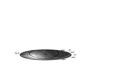
(a) (b) (c) (d)

Figure 2: Contour plots of the UHECR flux in equatorial coordinates for our four dark halo models, namely (a) cusped, (b) isothermal, (c) triaxial and (d) tilted. These are Hamer-Aitoff projections. The Galactic plane is marked in each figure. The effect of the halo of M31 is visible in the upper right of each plot.

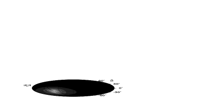
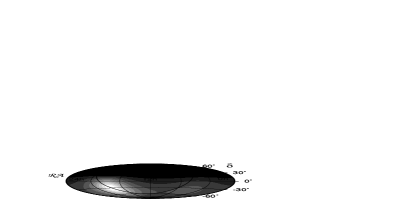
(a) (b) (c) (d)

Figure 3: As Figure 2, but now the UHECR flux has been convolved with the response in declination for the southern site of the Auger Observatory.

2.2 Harmonic Analysis

The strength and direction of the anisotropy in the arrival directions of the UHECRs can be quantified by harmonic analysis, as originally suggested by Linsley [l75 (46)]. The number of events is proportional to $N$, where:

$$N=\int d\delta\int d\alpha\,\cos\delta\,h(\delta)F(\alpha,\delta).$$ (11)

Let us define

$$a = {2\over N}\int d\delta\int d\alpha\,\cos\delta\cos\alpha\,h(\delta)F(\alpha,\delta),$$

$$b = {2\over N}\int d\delta\int d\alpha\,\cos\delta\sin\alpha\,h(\delta)F(\alpha,\delta),$$ (12)

so that the amplitude ${\cal R}$ and phase $\psi$ of the first harmonic is

$${\cal R}=(a^{2}+b^{2})^{1/2},\qquad\psi={\rm atan}\Biggl{(}{b\over a}\Biggr{)}.$$ (13)

Once we have a set of experimental UHECRs with amplitude ${\cal R}$ and phase $\psi$, the probability $P({\cal S},\vartheta)$ that this data came from a population characterized with an amplitude in $({\cal S},{\cal S}+d{\cal S})$ and phase $(\vartheta,\vartheta+d\vartheta)$ is given by [l75 (46)]

$$P({\cal S},\vartheta)=\frac{\sqrt{N}}{2\pi^{3/2}I_{0}(k_{0}/2)}\exp\Biggl{[}-{N\over 4}\Bigl{(}{\cal S}^{2}+{\textstyle\frac{1}{2}}{\cal R}^{2}-2{\cal R}{\cal S}\cos(\vartheta-\psi)\Bigr{)}\Biggr{]},$$ (14)

where $k_{0}={\textstyle\frac{1}{4}}{N{\cal R}^{2}}$ and $I_{0}$ denotes the zeroth order Bessel function of the first kind. Defining $\xi={\cal S}/{\cal R}$, then the differential probability distributions $P(\xi)$ and $P(\vartheta)$ are obtained by straightforward integration as

$$P(\xi) = {2k_{0}^{1/2}\over\pi^{1/2}I_{0}(k_{0}/2)}\exp\Bigl{[}-{k_{0}\over 2}(1+2\xi^{2})\Bigr{]}I_{0}\Bigl{(}{2k_{0}\xi}\Bigr{)},$$ (15)

$$P(\vartheta) = {1\over 2\pi I_{0}(k_{0}/2)}\Bigl{[}1\pm{\rm erf}\left[\pm k_{0}^{1/2}\cos(\vartheta-\psi)\right]\Bigr{]}\exp\Bigl{[}k_{0}(\cos^{2}(\vartheta-\psi)-{\textstyle\frac{1}{2}})\Bigr{]}.$$ (16)

Figure 1 shows these probability distributions. For large numbers of events, these distributions tend towards normal. It is not obvious that the assumption of normal distributions is appropriate for the AGASA and Haverah Park datasets, as the number of events is rather modest. In this paper, we always calculate the dispersions about the expected value corresponding to a given confidence limit by solving the integral equation over the distribution. For example, the dispersion $\sigma_{\vartheta}$ corresponding to the $95\%$ confidence limit is given by

$$\int_{\langle\vartheta\rangle-\sigma_{\vartheta}}^{\langle\vartheta\rangle+\sigma_{\vartheta}}P(\vartheta)d\vartheta=0.95.$$ (17)

The symmetric dispersion on the amplitude $\sigma_{\cal S}$ can be defined in the same way. However, the confidence limits on the amplitude ${\cal S}$ are asymmetric about the average values. So, sometimes it is useful to use asymmetric dispersions $\sigma_{\cal S}^{+}$ and $\sigma_{\cal S}^{-}$ corresponding to $95\%$ confidence limits defined via

$$\int_{\langle\xi\rangle}^{\langle\xi\rangle+\sigma_{\xi}^{+}}P(\xi)d\xi=0.475,$$ (18)

and

$$\int_{\langle\xi\rangle-\sigma_{\xi}^{-}}^{\langle\xi\rangle}P(\xi)d\xi=0.475.$$ (19)

Unless stated to the contrary, we use the asymmetric definitions of confidence limits for the amplitude. This distinction can be important at small $k_{0}$.

2.3 The Data

Table 1 summarises the available experimental data. The Haverah Park shower array detected 27 UHECRs with energies above $4\times 10^{19}$ eV and zenith angle less than $45^{\circ}$ [stanev (47)]. For the AGASA experiment, we use the data on the 57 UHECRs detected before May 2000 [agasa2 (27)]. Table 1 records the amplitude ${\cal R}$ and phase $\psi$ as determined from the two datasets. The $95\%$ confidence limits on the amplitude and phase are given, from which it is already evident that the presently available data are too sparse to claim a secure detection of any anisotropy. This is in accord with AGASA’s own analysis of the 47 events they observed before August 1998, in which they assert that there is no evidence for significant large-scale anisotropy on the celestial sphere.

Sommers [ps (44)] has estimated that the likely size of the dataset after 5 years of operation of the Auger Observatory is $\sim 2200$ events. This though is the combined total from both North and South Auger Observatories. In this paper, we are interested in the prospects over the next few years and so we restrict our analysis to South Auger. To give a feel for what it may achieve should there be a real anisotropy in the UHECR sky, we present two further examples in Table 1. In the first (henceforth Auger I), we assume that its amplitude and phase are the same as that indicated by AGASA, but that the number of events detected over $\sim 4\times 10^{19}$ eV is $1000$. In the second (Auger II), we assume the amplitude and phase are the same as that indicated by Haverah Park (which uses water-Cerenkov detectors of the same depth as Auger) and the number of post-GZK events is $1000$. In both cases, the size of even the $95\%$ confidence limits is reduced to typically $\sim 10^{\circ}$ in phase and $\sim 30\%$ in amplitude.

Table 2 gives the details of further tests for isotropy. We list the probability that an amplitude higher than that measured ${\cal R}$ can arise from an underlying isotropic distribution. This is given by the formula [l75 (46)]

$$P(>{\cal R})=\exp(-k_{0}).$$ (20)

We also give the probability that the data comes from a model with an amplitude ${\cal S}$ between 0 (isotropic) and the symmetric dispersion $\sigma_{\cal S}$ corresponding to the $68\%$ and $95\%$ confidence limits. This table underlines that the present AGASA and Haverah Park datasets are inadequate for the unambiguous identification of any anisotropy signal, if it exists. For example, an amplitude equal to or exceeding that reported by AGASA can come from an isotropic distribution with a probability exceeding a third, which is hardly negligible. The final two rows of Table 2 show the impact that South Auger will make. The small numbers for the probabilities demonstrate that genuine anisotropy signals with the same amplitude and phase as indicated by AGASA and Haverah Park will be convincingly detected.

(a) Isothermal (Extent of 250 kpc)

Field Size	$\Phi_{\rm M31}/\Phi_{\rm MW}$	$\Phi_{\rm M31}/\Phi_{\rm MW}$
	(Approx, eq. 26)	(Exact, eq. 27)
$2^{\circ}\times 2^{\circ}$	39.7	2.5
$10^{\circ}\times 10^{\circ}$	1.6	0.6
$15^{\circ}\times 15^{\circ}$	0.7	0.4

(b) Isothermal (Extent of 100 kpc)

Field Size	$\Phi_{\rm M31}/\Phi_{\rm MW}$	$\Phi_{\rm M31}/\Phi_{\rm MW}$
	(Approx, eq. 26)	(Exact, eq. 27)
$2^{\circ}\times 2^{\circ}$	16.4	2.6
$10^{\circ}\times 10^{\circ}$	0.7	0.5
$15^{\circ}\times 15^{\circ}$	0.3	0.3

(c) Cusped (Extent of 250 kpc)

Field Size	$\Phi_{\rm M31}/\Phi_{\rm MW}$	$\Phi_{\rm M31}/\Phi_{\rm MW}$
	(Approx, eq. 26)	(Exact, eq. 27)
$2^{\circ}\times 2^{\circ}$	18.1	3.0
$10^{\circ}\times 10^{\circ}$	0.7	0.4
$15^{\circ}\times 15^{\circ}$	0.3	0.2

(d) Cusped (Extent of 100 kpc)

Field Size	$\Phi_{\rm M31}/\Phi_{\rm MW}$	$\Phi_{\rm M31}/\Phi_{\rm MW}$
	(Approx, eq. 26)	(Exact, eq. 27)
$2^{\circ}\times 2^{\circ}$	11.8	3.0
$10^{\circ}\times 10^{\circ}$	0.5	0.4
$15^{\circ}\times 15^{\circ}$	0.2	0.2

Table 3: Ratio between incoming UHECR flux from the M31 halo to that from the Galaxy for fields of view of various sizes centered on M31. The second column shows the dangers of the point mass approximation, which overestimates the importance of the effect, while the third column gives the exact result. In tables (a) and (b), both galaxies are modelled with isothermal haloes, but with an extent 250 kpc and 100 kpc respectively. Tables (c) and (d) are the same but for the use of the cusped halo models, rather than isothermals.

3 The Dark Halo of the Galaxy

3.1 Models

There is little definite evidence on the structure of the Galaxy’s dark matter halo. The HI gas rotation curve of the Milky Way cannot be traced much beyond $\sim 20$ kpc. It is the kinematics of the distant satellite galaxies that provide the best evidence on the total mass and the extent of the Galaxy. The most recent estimate [mark (48)] finds a total mass $\sim 2\times 10^{12}$M_⊙ and an extent of $\gtrsim 200$ kpc. Such a large extent is in accord with earlier studies of the Milky Way and external spiral galaxies [zaritsky (49)].

N-body computer simulations of structure formation in hierarchical merging cosmogonies have provided evidence for a cusped density profile for dark haloes [nfw96 (22)]

$$n({\bf r})\propto\frac{1}{(r+r_{\epsilon})(r+r_{\rm s})^{2}},$$ (21)

where ${\bf r}$ is the position with respect to the Galactic Centre and $r=|{\bf r}|$ is the spherical polar radius. Here, $r_{\rm s}$ is the scale radius, which is typically $\sim 10$ kpc for the Galaxy, while $r_{\epsilon}$ is set by the resolution limit of the simulations, nowadays $\sim 0.5$ kpc. These models (hereafter NFW) have been much in vogue over the last few years. For example, they have already been used in calculations of the flux of UHECRs and the strength of the anisotropy signal [bsw99 (19, 20)]. The cusped density distribution of the NFW profile necessarily implies that the inner regions are dominated by dark matter and gives a substantial anisotropy signal. However, there are three reasons why the NFW is certainly incorrect for the Galaxy [york (50)]; first, the mass density implied by the luminous disk and bar is already sufficient to account for the rotation curve in the inner Galaxy without any contribution from dark matter [ortwin (51)]; second, numerical simulations of barred galaxies shows that copious amounts of dark matter in the inner parts slow down and rapidly dissolve bars through dynamical friction [victor (52)]; and third, the microlensing optical depth to the red clump stars already shows that almost all the density in the inner Galaxy must be in the form of compact objects capable of causing microlensing and so cannot be particle dark matter [jjb (53)].

It is more likely that the Galaxy’s dark halo has an isothermal distribution with a large core radius. Unlike the NFW profile, this at least satisfies one of the few pieces of secure evidence — namely that luminous matter dominates the central regions, whereas dark matter dominates the outer parts. As a prototype of this model, we take the cored isothermal-like sphere [nwe (54)]

$$n({\bf r})\propto\frac{3r_{\rm c}^{2}+r^{2}}{(r_{\rm c}^{2}+r^{2})^{2}}.$$ (22)

Here, $r_{\rm c}$ is the core radius, which is chosen to be $\sim 10$ kpc. This parameter is not constrained at all by the observations, but its precise value does not have a big effect on the anisotropy of the UHECRs. The model is the spherical limit of a more general family of triaxial density distributions [wyn (55)]

$$n({\bf r})\propto\frac{Ax^{2}\!+\!By^{2}\!+\!Cz^{2}\!+\!D}{(r_{\rm c}^{2}\!+\!x^{2}\!+\!y^{2}p^{-2}\!+\!z^{2}q^{-2})^{2}},$$ (23)

where ${\bf r}=(x,y,z)$ and the constants $A,B,C$ and $D$ are

$$A=(p^{-2}\!+\!q^{-2}\!-\!1),\quad B=p^{-2}(1\!-\!p^{-2}\!+\!q^{-2}),\quad C=q^{-2}(1\!+\!p^{-2}\!-\!q^{-2}),\quad D=r_{\rm c}^{2}(1\!+\!p^{-2}\!+\!q^{-2}).$$ (24)

Here, $p$ and $q$ are axis ratios of the potential. When $p=1$, the halo is oblate, whilst when $p=q$, the halo is prolate. The shape of the Galaxy’s dark halo is uncertain. The flaring of the outer HI gas disk does provide direct evidence on the vertical force at the midplane from the halo, which is greater for flattened models. Analyses of this effect have been used to determine the shape of the halo [OM (56)], but they are hampered by the unknown contribution to pressure support from magnetic fields and cosmic rays at large distances from the Sun. There is also evidence on the shape of the halo from stellar kinematics [rpvdm (57)], although this is beset with modelling uncertainties as to the orientation of the velocity ellipsoid. Such evidence as there is suggests a flattened dark halo with an ellipticity less than E7. However, even though evidence on the shape of the dark halo is sparse, it is natural to expect halos built from merging and accretion to possess flattened, generically triaxial, shapes rather than spherical ones [warren (58)]. For the sake of definiteness, we take $p=0.9$ and $q=0.75$, which means that the density contours have semi-axes in the ratio $1:0.788:0.428$. This is a highly flattened model with an ellipticity  of roughly E6. At first glance, a triaxial halo may seem to afford a great deal of freedom as to the location of the Sun. This is of course not the case! The Sun must be located close to one of the principal axes, as otherwise there would be gross differences between the Galaxy as viewed at positive and negative longitudes. Both local and global dynamical evidence favour the location of the Sun as close to (within $10^{\circ}$ of) the major axis of the Galactic disk [kt (59)].

There is one other effect that may be common. It has been emphasised [james (60)] that the outer parts of the dark halo may be misaligned with the disk. This is one possible cause of the phenomenon of warping of the neutral gas disk, an effect that is known to be present in the outer Milky Way. A family of tilted halo models has density

$$n({R^{\prime}},{z^{\prime}})\propto\frac{r_{\rm c}^{2}(2\!+\!q^{-2})\!+\!q^{-2}{R^{\prime}}^{2}\!+\!{z^{\prime}}^{2}q^{-2}(2\!-\!q^{-2})}{(r_{\rm c}^{2}\!+\!{R^{\prime}}^{2}\!+\!{z^{\prime}}^{2}q^{-2})^{2}},$$ (25)

where ${R^{\prime}}^{2}={x^{\prime}}^{2}+{y^{\prime}}^{2}$. The coordinates (${x^{\prime}},{y^{\prime}},{z^{\prime}}$) are related to ($x,y,z$) by a rotation through an angle $\theta$ about the $x$-axis, on which the Sun lies. The motivation for this is that the Sun lies nearly on the line of nodes of the warp. We take $\theta=30^{\circ}$, an extreme value, as we are interested in the qualitative effects of tilted haloes.

There are two astrophysical parameters we will need to calculate signatures of the UHECRs, assuming they arise from the decay of heavy relics in the halo. The first is ${\bf R_{\odot}}$, the distance from the Sun to the Galactic Centre, which is taken as $(8.5,0,0)$ [kerr (61)]. The second is ${r_{\rm max}}$, the extent of the halo, which is taken as $\sim 250$ kpc in accord with the most recent estimates [mark (48, 49)]. The halo extent is poorly known and results depending sensitively on this parameter must be viewed with some caution.

\psfrag{r}{${\cal S}$}\psfrag{p}{$\vartheta$}\includegraphics[width=199.16928pt,height=199.16928pt]{./final_fig4a.eps}	\psfrag{r}{${\cal S}$}\psfrag{p}{$\vartheta$}\includegraphics[width=199.16928pt,height=199.16928pt]{./final_fig4b.eps}
(a)	(b)
\psfrag{r}{${\cal S}$}\psfrag{p}{$\vartheta$}\includegraphics[width=199.16928pt,height=199.16928pt]{./final_fig4c.eps}	\psfrag{r}{${\cal S}$}\psfrag{p}{$\vartheta$}\includegraphics[width=199.16928pt,height=199.16928pt]{./final_fig4d.eps}
(c)	(d)

Figure 4: Plots of the amplitude against the phase for the four models (cusped, isothermal, triaxial and tilted). Also shown are the $95\%$ confidence limits for (a) the AGASA and (b) the Haverah Park experiments. The lower panels show the expected impact of South Auger. Marked are the $95\%$ confidence limits assuming the amplitude and phase of (c) the AGASA and (d) the Haverah park experiments, but with 1000 events.

3.2 Results

Figure 2 shows what our four halo models look like in the cosmic ray sky. These are contours of the incoming UHECR flux in equatorial coordinates. Figure 3 shows the contours convolved with the response function $h_{1}(\delta)$ for South Auger. (The figure for $h_{2}(\delta)$ is very similar). If the UHECRs do originate in dark haloes, then the halo of the nearby Andromeda galaxy (M31) may give a tell-tale signature. M31 is the only other large galaxy in the Local Group, and it is roughly as massive as the Galaxy [ewggv (62)]. The halo of M31 is modelled as an isothermal sphere centered 770 kpc away and with an extent of $250$ kpc. In Figures 2 and 3, the hotspot at $\alpha_{0}\approx 00^{\rm h}43^{\rm m},\delta_{0}\approx 41^{\circ}$ (referred to the J2000.0 epoch) is caused by M31. It has already been claimed that the absence of a hotspot in the data rules out the decaying dark matter origin of UHECRs [bsw99 (19)], though this has been contested by others [mtw99 (20)].

The issue is worth considering in more detail. The ratio of the mass of M31 to that of the Galaxy used previously [bsw99 (19, 20)] is two to one. There is little dynamical evidence for such a ratio. The asymptotic rotation curve of M31 is just $\sim 10\%$ higher than that of the Galaxy. The most reliable estimate for the mass of the M31 halo based on the motions of satellite galaxies, planetary nebulae and globular clusters is $\sim 1\times 10^{12}\,{\rm M}_{\odot}$, though there is at least a factor of two uncertainty in this value due to the small sizes of the tracer datasets [ewggv (62)]. On balance, it is probably more accurate to assume that M31 is roughly as massive as the Galaxy. Now, to compute the ratio of the total flux received from M31 to that received from the Milky Way $\Phi_{\rm M31}/\Phi_{\rm MW}$, the following expression has sometimes been used [mtw99 (20)]:

$$\frac{\Phi_{\rm M31}}{\Phi_{\rm MW}}\sim\frac{\xi}{D^{2}}\times\frac{\int_{V_{\rm M31}}n_{\rm M31}\,dV}{\int_{V_{\delta\Omega}}n_{\rm MW}/r^{2}\,dV}.$$ (26)

Here, $\xi$ is the ratio between the masses of the two haloes, $D\sim 770$ kpc, $V_{\rm M31}$ is the volume of the halo of M31 and $V_{\delta\Omega}$ is the volume defined by the cone of solid angle $\delta\Omega$ pointing towards M31. There are two drawbacks to this formula. First, it assumes that M31 is point-like so that $n_{\rm M31}/r^{2}$ is taken as constant and equal to its value at the center of M31. Second, it assumes that the entire halo of M31 fits into the angular window. Accordingly, we prefer to use the exact expression

$$\frac{\Phi_{\rm M31}}{\Phi_{\rm MW}}\sim\frac{\int_{\alpha_{0}-\Delta\alpha/2}^{\alpha_{0}+\Delta\alpha/2}\,d\alpha\int_{\delta_{0}-\Delta\delta/2}^{\delta_{0}+\Delta\delta/2}\cos\delta\,d\delta\int_{s_{-}}^{s_{+}}n_{\rm M31}\,ds}{\int_{\alpha_{0}-\Delta\alpha/2}^{\alpha_{0}+\Delta\alpha/2}\,d\alpha\int_{\delta_{0}-\Delta\delta/2}^{\delta_{0}+\Delta\delta/2}\cos\delta\,d\delta\int_{0}^{s_{\rm max}}n_{\rm MW}\,ds}.$$ (27)

Here, the flux ratio is measured in an angular window $\Delta\alpha\times\Delta\delta$ centered on the right ascension $\alpha_{0}$ and declination $\delta_{0}$ of M31. The quantities $s_{\pm}$ are computed by finding the intersection of the line of sight towards with a sphere of radius $250$ kpc, while $s_{\rm max}$ is the usual limit of the Galaxy halo. Both the Galaxy and M31 are modelled with identical cored isothermal haloes. Table 3 gives the results for the flux ratio computed using the approximate formula (26) and the exact one (27). Results are presented when both the Galaxy and M31 are modelled with isothermal and cusped haloes of extents of 250 kpc and 100 kpc. We see that the effects of an extended dark halo are not always well-represented by the point-like approximation. However, formula (26) is still valuable, as it gives an upper limit to M31’s contribution. Given that the expected spread caused by the deflection of a $4\times 10^{19}$ eV proton originating from Andromeda is of the order of a few degrees, a field of view of $10^{\circ}\times 10^{\circ}$ is probably the most appropriate one to look for the enhancement effect of the M31 halo [mtw99 (20)]. On such scales, no substantial enhancement effect is expected and the dominant source of UHECRs remains the Galaxy.We therefore agree with the assessment of Medina Tanco & Watson [mtw99 (20)] – and disagree with Benson et al. [bsw99 (19)] – as regards the visibility of M31 in the UHECR sky.

(a) AGASA

Model	Amplitude	Phase	$P(\sigma_{\cal S},\sigma_{\vartheta})$	$P(\sigma_{\cal S})$	$P(\sigma_{\vartheta})$
	${\cal S}$	$\vartheta$	$(95\%)$	$(95\%)$	$(95\%)$
Cusped	0.497	265.8	0.328	0.330	0.944
Isothermal	0.385	265.8	0.563	0.572	0.944
Triaxial	0.251	295.0	0.865	0.898	0.950
Tilted	0.346	267.8	0.651	0.665	0.945

(b) Haverah Park

Model	Amplitude	Phase	$P(\sigma_{\cal S},\sigma_{\vartheta})$	$P(\sigma_{\cal S})$	$P(\sigma_{\vartheta})$
	${\cal S}$	$\vartheta$	$(95\%)$	$(95\%)$	$(95\%)$
Cusped	0.446	265.8	0.530	0.977	0.543
Isothermal	0.350	265.8	0.515	0.951	0.542
Triaxial	0.224	301.2	0.172	0.887	0.180
Tilted	0.314	268.2	0.480	0.937	0.513

Table 4: For each of the models, the theoretical values of the amplitude and the phase are calculated using the response functions for (a) AGASA and (b) Haverah Park. We also give the probabilities that the experimental amplitude and phase come from within the $95\%$ confidence limits of the model.

(a) Auger I

Model	$P(\sigma_{\cal S},\sigma_{\vartheta})$	$P(\sigma_{\cal S})$	$P(\sigma_{\vartheta})$
	($95\%$)	($95\%$)	($95\%$)
Cusped	$<10^{-3}$	$<10^{-3}$	$0.095$
Isothermal	$0.014$	0.202	0.095
Triaxial	0.886	0.950	0.932
Tilted	0.059	0.509	0.133

(b) Auger II

Model	$P(\sigma_{\cal S},\sigma_{\vartheta})$	$P(\sigma_{\cal S})$	$P(\sigma_{\vartheta})$
	($95\%$)	($95\%$)	($95\%$)
Cusped	$<10^{-3}$	$0.156$	$<10^{-3}$
Isothermal	$<10^{-3}$	$0.001$	$<10^{-3}$

(c) Predictions for South Auger

Model	Amplitude	Phase	Amplitude	Phase
	$(h_{1})$	$(h_{1})$	$(h_{2})$	$(h_{2})$
Cusped	0.883	265.8	0.806	265.8
Isothermal	0.558	265.8	0.508	265.8
Triaxial	0.551	257.9	0.508	255.9
Tilted	0.512	265.0	0.457	264.6

Table 5: For each of the models, this gives an idea of what we will learn from the southern station of the Auger Observatory. Table (a) assumes the amplitude and phase of the AGASA experiment, table (b) the amplitude and phase from Haverah Park; in both cases, 1000 events are analysed as typical of the number of UHECRs recorded by South Auger. In Table (b), only the results for the isothermal and cusped models are recorded; for the other models, all the probabilities are less than $10^{-3}$. Table (c) presents the predictions for our halo models using the two possible response functions $h_{1}(\delta)$ and $h_{2}(\delta)$.

Table 4 examines the four halo models (cusped, isothermal, triaxial and tilted). For the moment, we assume the canonical values of the halo parameters given in Section 3.1. For each model, we compute the theoretical amplitude ${\cal S}$ and phase $\vartheta$ in the first two columns. Then, the next columns give the probability that the experimental data came from a particular model with ${\cal S}$ in $({\cal S}-\sigma_{\cal S},{\cal S}+\sigma_{\cal S})$ and $\vartheta$ in $(\vartheta-\sigma_{\vartheta},\vartheta+\sigma_{\vartheta})$. This is found by computing the integral

$$P(\sigma_{S},\sigma_{\vartheta})=\int_{{\cal S}-\sigma_{\cal S}^{-}}^{{\cal S}+\sigma_{\cal S}^{+}}\int_{\vartheta-\sigma_{\vartheta}}^{\vartheta+\sigma_{\vartheta}}{P({\cal S},\vartheta)d{\cal S}d\vartheta}.$$ (28)

The final two columns give the equivalent results for the one-dimensional distributions of amplitude and phase.

For both AGASA and Haverah Park response functions, the amplitude is greatest for the cusped NFW model. This makes good sense, as this model has the largest central density. We have argued above that the Galaxy almost certainly does not have such a cusped density distribution for its dark halo, and so a better guide to the expected amplitude is provided by the other three halo models. Isothermal-like models with a core radius $\sim 10$ kpc have an anisotropy of amplitude ${\cal S}\lesssim 0.4$ as measured by the AGASA and Haverah Park experiments. For all four models, the phase points roughly towards the Galactic Centre at $\alpha\approx 17^{\rm h}45^{\rm m},\delta\approx-29^{\circ}$. The largest deviation from this direction of $35^{\circ}$ occurs for the triaxial halo. Notice that the probabilities listed in the final three columns are all far from insignificant. The data are compatible with any of the models. The present dataset is insufficient to discriminate between possible dark matter halo densities.

In Table 5 (a), which corresponds to Auger I, we see the improvement in discrimination. The amplitude and phase is the same as that seen by AGASA (see Table 1) and happens to lie close to the prediction of the triaxial model. Hence, Table 5 (a) shows that all the probabilities are very small, except that of the triaxial model. In other words, there is now successful discrimination between halo models. All the probabilities in Table 5 (b), which corresponds to Auger II, are very small. The phase, assumed to be that of Haverah Park, does not lie close to any of the halo models which are accordingly ruled out. In Table 5 (c), we give the expected amplitude and phase for our four halo models and convolved with the two different response functions $h_{1}(\delta)$ and $h_{2}(\delta)$ proposed for South Auger. These results are shown pictorially in Figure 4. The panels show the datasets from AGASA, Haverah Park, Auger I and II, together with $95\%$ confidence limits.

The anisotropy of all four halo models has a larger amplitude (${\cal S}\gtrsim 0.5$) at the South Auger detector ($35^{\circ}$ S) than at AGASA ($36^{\circ}$ N) or Haverah Park ($54^{\circ}$ N). For the spherical models, the phase marks the direction of the Galactic Centre. A signature of triaxiality is that the phase has different angular offsets from the Galactic Centre direction at different detector locations.

Figure 5 investigates the amplitude ${\cal S}$ and phase $\vartheta$ seen by South Auger as a function of the model parameters for the four halo models. Panels (a) and (b) show the effects of varying the scale radius $r_{\rm s}$ of the cusped NFW halo and the core radius $r_{\rm c}$ of the isothermal halo. These parameters affect only the amplitude of the harmonic and not the phase, which is always in the direction of the Galactic Centre. Note that there is no simple way of measuring the core radius of a dark halo from astrophysical data. Usually, the core radius is inferred by least-square fitting to the galaxy rotation curve, but this is an uncertain procedure as a single rotation curve must be decomposed into separate contributions from the bulge, disk and halo. If UHECRs are indeed produced by decaying dark matter, these plots raise the exciting possibility that halo core radius may become directly accessible to measurement. During the first 5 years of operation of South Auger, the core radius could be measured if $r_{\rm c}\lesssim 10$ kpc. Panel (c) shows the effect of varying the shape of the triaxial halo. The oblate models ($p=1$) show largest deviation in phase ($\sim 15^{\circ}$) from the spherical model ($p=q=1$). By comparison, stretching or flattening the halo does not change the value of the amplitude ${\cal S}$ by much. In panel (d), the tilt angle is varied. This can give large deviations in phase ($\sim 25^{\circ}$) and significant changes in amplitude. Overall, Figure 5 suggests the shape of the halo controls the phase $\vartheta$, whereas the scale of the halo controls the amplitude ${\cal S}$.

Figure 6 shows the the number of events ${\cal N}_{\cal S}$ required for a convincing $5\sigma$ detection of the anisotropy signal for the four halo models at South Auger. An approximate method is to use

$${\cal N}_{\cal S}\approx{2n_{\sigma}^{2}\over{\cal S}^{2}}.$$ (29)

This gives the number of events required for a signal-to-noise ratio of $n_{\sigma}$ standard deviations in amplitude. This assumes that the probability density $P({\cal S})$ is a normal distribution about ${\cal S}={\cal R}$ with dispersion equal to $\sqrt{2/{\cal N}_{\cal S}}$. This is not the case, especially when the number of events is small or the amplitude is small (i.e., $k_{0}$ is small). In an exact calculation, the signal-to-noise is computed from its definition

$$n_{\sigma}\equiv\frac{\langle{\cal S}\rangle}{\sqrt{\sigma_{\cal S}^{2}}},$$ (30)

where

$$\langle{\cal S}\rangle\equiv\int_{0}^{\infty}d{\cal S}\,{\cal S}P({\cal S}),\qquad\qquad\sigma_{\cal S}^{2}\equiv\left\{\int_{0}^{\infty}d\,{\cal S}{\cal S}^{2}P({\cal S})\right\}-\langle{\cal S}\rangle^{2}.$$

If we fix $n_{\sigma}=5$, as is required for a convincing detection, then eq. (30) is an implicit equation for ${\cal N}_{\cal S}$, which can be solved iteratively. Figure 6 (a) and (b) show the number of events for a $5\sigma$ detection calculated using the exact expression (full curves) and the normal approximation (dashed curves), from which it is evident that the approximation tends to underestimate the required number of events. Nonetheless, given the ease with which the normal approximation can be computed, it is reassuring to see that it is never seriously in error. Roughly 40 events may be needed if the Galaxy’s halo has a cusped NFW profile with a small scale length $r_{\rm s}<2$ kpc. More likely, if the halo is an isothermal sphere with large core radii ($r_{\rm c}\sim 10-20$ kpc), then typically 150-500 events may be required. Thus, within 5 years of operation, South Auger will be able to rule some halo models out.

Panels (c) and (d) show that shape parameters like triaxiality and tilt do not have a substantial influence on the number of required events for a convincing measurement of the amplitude. For these models, it is more interesting to ask how many events $N_{\varphi}$ are needed for the error bars on the phase to be reduced to $\pm\beta$. Using the normal approximation, this gives

$${\cal N}_{\varphi}\approx{2n_{\sigma}^{2}\over{\cal S}^{2}}{1\over\sin^{2}\beta}.$$ (31)

For example, for the $3\sigma$ error bars on the phase measured at South Auger to be reduced to $\pm 10^{\circ}$ requires $\sim 2000$ events. This is the number needed to begin to distinguish between different triaxial or tilted models and is possible after $\gtrsim 10$ years of operation. A less ambitious target is to ask for the $3\sigma$ error bars to be $\pm 20^{\circ}$, which requires $\sim 500$ events. This is ample to verify that the phase points in the rough direction of the Galactic Centre and thus implicate the decaying dark matter models as the correct mechanism for UHECR production.

\psfrag{r}{${\cal S}$}\psfrag{p}{$\vartheta$}\psfrag{b}{$\scriptstyle r_{\rm s}=100\,{\rm kpc}$}\psfrag{s}{$\scriptstyle r_{\rm s}=1\,{\rm kpc}$}\includegraphics[width=184.9429pt,height=170.71652pt]{./final_fig5a.eps}	\psfrag{r}{${\cal S}$}\psfrag{p}{$\vartheta$}\psfrag{b}{$\scriptstyle r_{\rm c}=100\,{\rm kpc}$}\psfrag{s}{$\scriptstyle r_{\rm c}=1\,{\rm kpc}$}\includegraphics[width=184.9429pt,height=170.71652pt]{./final_fig5b.eps}
(a)	(b)
\psfrag{r}{${\cal S}$}\psfrag{p}{$\vartheta$}\psfrag{h}{$\scriptstyle p=q$}\psfrag{l}{$\scriptstyle p=1$}\includegraphics[width=184.9429pt,height=170.71652pt]{./final_fig5c.eps}	\psfrag{r}{${\cal S}$}\psfrag{p}{$\vartheta$}\psfrag{a}{$\scriptstyle\theta=40^{\circ}$}\psfrag{b}{$\scriptstyle\theta=-40^{\circ}$}\includegraphics[width=184.9429pt,height=170.71652pt]{./final_fig5d.eps}
(c)	(d)

Figure 5: Amplitude-phase plots showing how the anisotropy signal measured by South Auger varies with the parameters in the (a) cusped, (b) isothermal, (c) triaxial and (d) tilted halo models. The legend in (c) and (d) corresponds to the flattening in the potential $q$.

\psfrag{r}{$r_{\rm s}$}\psfrag{p}{$\!\!\!\!\!\!\!\!{\cal N}_{\cal S}$}\includegraphics[width=184.9429pt,height=170.71652pt]{./final_fig6a.eps}	\psfrag{r}{$r_{\rm c}$}\psfrag{p}{$\!\!\!\!\!\!\!\!{\cal N}_{\cal S}$}\includegraphics[width=184.9429pt,height=170.71652pt]{./final_fig6b.eps}
(a)	(b)
\psfrag{r}{$p$}\psfrag{p}{$\!\!\!\!\!\!\!\!{\cal N}_{\cal S}$}\includegraphics[width=184.9429pt,height=170.71652pt]{./final_fig6c.eps}	\psfrag{r}{$\theta$}\psfrag{p}{$\!\!\!\!\!\!\!\!{\cal N}_{\cal S}$}\includegraphics[width=184.9429pt,height=170.71652pt]{./final_fig6d.eps}
(c)	(d)

Figure 6: Number of events required for 5$\sigma$ detection of an anisotropy by South Auger for the (a) cusped, (b) isothermal, (c) triaxial and (d) tilted halo models. The full and dashed curves in (a) and (b) refer to the exact result and the normal approximation respectively. The legend in (c) and (d) corresponds to the flattening in the potential $q$.

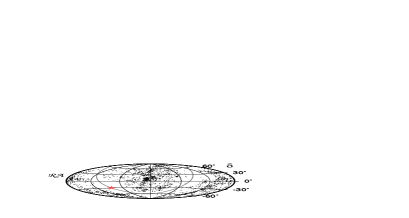
(a)	(b)
(c)	(d)

Figure 7: Hammer-Aitoff projections in equatorial coordinates-s of the four samples of galaxies, namely (a) Sample I, (b) Sample II, (c) Sample III and (d) Sample IV. These plots record the positions of the galaxies, not the flux of incoming UHECRs. The Galactic Center is marked with a star.

4 Nearby Extragalactic Sources

4.1 Models

There are two serious impediments to the proposal that extragalactic sources supply the UHECRs. First, most of the UHECRs do not point back towards any obvious astrophysical sources, such as the active or interacting galaxies within $\sim 50$ Mpc. For example, the possible source of the highest energy Fly’s Eye event was examined in [es95 (24)] and the best candidate amongst nearby sources was the starburst galaxy M82, some $37^{\circ}$ away. Second, the possibilities for acceleration of cosmic rays to such extreme energies in any extragalactic object seem to be intrinsically limited [egsource (63)]. Despite the obstacles, the idea that UHECRs originate in extragalactic sources is still worth examining. At energies exceeding $E\sim 4\times 10^{19}$ eV, the UHECRs in the Haverah Park dataset exhibit a correlation with the direction of the supergalactic plane [stanev (47)], though this is not seen in the AGASA experiment [hayashida (41)]. However, two of the AGASA clusters (C1 and C2) do lie close to the supergalactic plane and do have tentative identifications with nearby galaxies.

Let us suppose that supermassive black holes in galactic nuclei produce UHECRs. There is increasing evidence that many, perhaps all, galaxies contain central black holes, even if their nuclei display only low levels of activity today. Very convincing candidates are provided by the nearby galaxy NGC 4258, where maser emission has traced out the gas cloud motions around a central black hole of $\sim 3.6\times 10^{7}\,{\rm M}_{\odot}$, as well as the Galaxy, where the proper motions of stars very close to the center strongly suggest a black hole of mass $\sim 2\times 10^{6}\,{\rm M}_{\odot}$ [rees2 (64)]. Stellar kinematics can now be obtained at high spatial resolution (down to $1^{\prime\prime}$) with the new generation of spectrographs, enabling the nuclear regions of nearby galaxies to be probed. This has strengthened the evidence for supermassive black holes in a number of nearby galaxies, such as M31, M32 and M87 [richstone (65)]. The case of M32 is particularly interesting. Although it is only a low luminosity galaxy, there is strong evidence for a supermassive black hole of $\sim 2\times 10^{6}\,{\rm M}_{\odot}$ [m32 (66)]. Only its relative closeness enables the black hole to be identified.

The Third Reference Catalogue of Bright Galaxies (RC3) is reasonably complete for nearby galaxies [devauc (67)]. It aims to include all galaxies with total B-band magnitudes $B_{\rm T}$ brighter than $\sim 15.5$ and with a redshift less than $15000$ kms^-1. We use it to construct the following datasets. Samples I and II contain all galaxies in the RC3 intrinsically brighter than M32 (NGC 221) and closer than 50 Mpc and 100 Mpc respectively. M32 is the smallest galaxy for which there is good evidence for a central black hole, so it is a reasonable supposition that all galaxies larger than M32 contain black holes, even if quiescent. Samples III and IV contains all galaxies in the RC3 intrinsically brighter than Centaurus A (NGC 5128) and closer than 50 Mpc and 100 Mpc respectively. Centaurus A is the nearest active galaxy, so these Samples contain only the brightest and largest of the nearby galaxies.

The motivation behind these choices is to answer the following questions. What is the expected anisotropy signal if only big, bright galaxies supply the UHECRs, or if all nearby galaxies contribute equally? Is it only galaxies within 50 Mpc that dominate the signal?

(a) AGASA

Model	Amplitude	Phase	$P(\sigma_{\cal S},\sigma_{\vartheta})$	$P(\sigma_{\cal S})$	$P(\sigma_{\vartheta})$
	${\cal S}$	$\vartheta$	$(95\%)$	$(95\%)$	$(95\%)$
Sample I	0.309	$111.1^{\circ}$	0.343	0.755	0.523
Sample II	0.307	$110.9^{\circ}$	0.346	0.759	0.524
Sample III	1.902	$10.7^{\circ}$	$<10^{-3}$	$<10^{-3}$	0.910
Sample IV	1.862	$10.9^{\circ}$	$<10^{-3}$	$<10^{-3}$	0.910

(b) Haverah Park

Model	Amplitude	Phase	$P(\sigma_{\cal S},\sigma_{\vartheta})$	$P(\sigma_{\cal S})$	$P(\sigma_{\vartheta})$
	${\cal S}$	$\vartheta$	$(95\%)$	$(95\%)$	$(95\%)$
Sample I	0.353	$110.8^{\circ}$	0.783	0.952	0.828
Sample II	0.352	$110.7^{\circ}$	0.782	0.952	0.828
Sample III	1.922	$10.8^{\circ}$	$<10^{-3}$	$<10^{-3}$	0.072
Sample IV	1.887	$10.9^{\circ}$	$<10^{-3}$	$<10^{-3}$	0.072

Table 6: For each of the four samples, the theoretical values of the amplitude and the phase are calculated using the response functions for (a) AGASA and (b) Haverah Park. We also give the probabilities that the experimental amplitude and phase come from within the $95\%$ confidence limits of the model.

(a) Auger I

Model	$P(\sigma_{\cal S},\sigma_{\vartheta})$	$P(\sigma_{\cal S})$	$P(\sigma_{\vartheta})$
	($95\%$)	($95\%$)	($95\%$)
Sample I	$<10^{-3}$	$0.801$	$<10^{-3}$
Sample II	$<10^{-3}$	$0.811$	$<10^{-3}$

(b) Auger II

Model	$P(\sigma_{\cal S},\sigma_{\vartheta})$	$P(\sigma_{\cal S})$	$P(\sigma_{\vartheta})$
	($95\%$)	($95\%$)	($95\%$)
Sample I	$<10^{-3}$	$0.001$	$<10^{-3}$
Sample II	$<10^{-3}$	$0.001$	$<10^{-3}$

(c) Predictions for South Auger

Model	Amplitude	Phase	Amplitude	Phase
	$(h_{1})$	$(h_{1})$	$(h_{2})$	$(h_{2})$
Sample I	0.471	$49.4^{\circ}$	1.187	$22.4^{\circ}$
Sample II	0.469	$48.7^{\circ}$	1.178	$22.3^{\circ}$
Sample III	0.568	$123.2^{\circ}$	1.395	$85.5^{\circ}$
Sample IV	0.411	$116.0^{\circ}$	1.268	$83.9^{\circ}$

Table 7: For each of the Samples, this shows the impact of the South Auger Observatory. Table (a) assumes the amplitude and phase of the AGASA experiment, table (b) the amplitude and phase from Haverah Park; in both cases, 1000 events are analysed. In Tables (a) and (b), lines are omitted if all the probabilities vanish. Table (c) presents the predictions for our four Samples using the two possible response functions $h_{1}(\delta)$ and $h_{2}(\delta)$.

\psfrag{r}{${\cal S}$}\psfrag{p}{$\vartheta$}\includegraphics[width=199.16928pt,height=199.16928pt]{./final_fig8a.eps}	\psfrag{r}{${\cal S}$}\psfrag{p}{$\vartheta$}\includegraphics[width=199.16928pt,height=199.16928pt]{./final_fig8b.eps}
(a)	(b)
\psfrag{r}{${\cal S}$}\psfrag{p}{$\vartheta$}\includegraphics[width=199.16928pt,height=199.16928pt]{./final_fig8c.eps}	\psfrag{r}{${\cal S}$}\psfrag{p}{$\vartheta$}\includegraphics[width=199.16928pt,height=199.16928pt]{./final_fig8d.eps}
(c)	(d)

Figure 8: Plots of the amplitude against the phase for the four Samples of galaxies. Also shown are the $95\%$ confidence limits for (a) the AGASA and (b) the Haverah Park experiments. The lower panels show the expected impact of South Auger. Marked are the $95\%$ confidence limits assuming the amplitude and phase of (c) the AGASA and (d) the Haverah Park experiments, but with 1000 events.

4.2 Results

To take into account the declinations of the galaxies, we use the discrete analogue-s of equations (11) and  (2.2):

$$N=\sum_{i}h(\delta_{i}){1\over r_{i}^{2}},$$ (32)

$$a=\frac{2}{N}\sum_{i}h(\delta_{i}){\cos\alpha_{i}\over r_{i}^{2}},\qquad b=\frac{2}{N}\sum_{i}h(\delta_{i}){\sin\alpha_{i}\over r_{i}^{2}},$$ (33)

where the index $i$ runs along all the galaxies in the Sample and $h(\delta)$ is the response function of each experiment.

Figure 7 shows the distribution of galaxies in the four Samples. The supergalactic plane is clearly visible, as is the Zone of Avoidance within $\sim 15^{\circ}$ of the Galactic plane. Some of the prominent local features are also readily apparent. The Virgo cluster is centered at $\alpha\approx 12^{\rm h}30^{\rm m},\delta\approx 10^{\circ}$, while the Fornax cluster is at $\alpha\approx 3^{\rm h},\delta\approx-40^{\circ}$. The densest part of the Local Supercluster and the Hydra-Centaurus supercluster are prominent at $\alpha\approx 12^{\rm h}-1^{\rm h},\delta\approx-40^{\circ}$, while the Perseus-Pisces cluster stretches from $\alpha\approx 1^{\rm h}-3^{\rm h},\delta\approx 40^{\circ}$. Of course, any optically selected survey is strongly affected by extinction at low Galactic latitudes. We could avoid this bias by using a different catalogue such as the IRAS galaxies. This though merely substitutes one bias for another, as early-type galaxies are under-represented in the IRAS survey, whereas late-type dusty disk galaxies are over-represented. How serious is the bias caused by low latitude extinction on our calculations? Let us note that the Dwingeloo Obscured Galaxy Survey conducted a shallow search in the entire Northern Zone of Avoidance for nearby and/or massive galaxies and this yielded just 5 candidates [dwingeloo (68)]. They estimated that there are $\sim 100$ galaxies missing within $\sim 50$ Mpc. The distance factors in eqs. (32,33) mean that the nearest galaxies have the largest weight. Hence, this suggests that low latitude obscuration will not have a deleterious effect on our results. Only if there are large numbers of missing galaxies within 10 Mpc is our calculation likely to be in error, and this circumstance does not seem to be the case, as judged by the available evidence.

Table 6 shows the signal expected for AGASA and Haverah Park. For all four Samples, the size of the amplitude is significant, so that detection of the anisotropy is not enough to implicate decaying dark matter haloes. Samples I and II, which contain almost all the nearby galaxies, do yield an anisotropic signal of the same order of magnitude as seen by AGASA and Haverah Park. In fact, the direction of the signal is well within the $95\%$ confidence limits for the Haverah Park dataset. The probabilities that the AGASA and Haverah Park datasets are drawn from within the $95\%$ confidence limits of the model are moderate ($0.264$) and high ($0.858$) respectively. The phase of the anisotropy is robust against changes in the cut-off radius, suggesting that it is the very closest galaxies (within $\sim 20$ Mpc) that are contributing most of the signal. The direction of the signal shows that it is is dominated by nearby structures in the supergalactic plane, especially the Virgo cluster. Of all our models, Samples III and IV, which contain the nearby bright galaxies within 50 and 100 Mpc respectively, give the largest amplitude for the anisotropy signal. They are clearly disfavored by the existing AGASA and Haverah Park datasets. Table 6 shows there is vanishingly small probability that either dataset is drawn from within the $95\%$ confidence limits of the model. The observed distribution of UHECRs seems to be more isotropic than expected if they emanate just from the nearby bright galaxies.

Table 7 shows the potential effects of the Auger Observatory. Again, Auger I has the same amplitude and phase as recorded by AGASA, while Auger II is the same as that recorded by Haverah Park, with the number of events increased to 1000. Of course, if UHECRs originate in nearby galaxies, then the Northern hemisphere signal will be different from the Southern hemisphere. We are simply resizing the experimental box to match Auger’s sensitivity as an illustration of its ability to discriminate. Tables 7 (a) and (b) are composed mainly of zeros. The large number of events now enables all four Samples to be ruled out, as the signals do not coincide with those measured by AGASA and Haverah Park. Figure 8 shows these results pictorially, together with the $95\%$ confidence limits.

The signal seen by South Auger is recorded in Table 7 (c). The amplitude is greater than that seen by the Northern Hemisphere detectors, and the phase points in a different direction. For Samples I and II, we obtain results that depend on the assumed detector response so it is difficult to make definite predictions. The number of events for a $5\sigma$ detection in the amplitude is $\sim 120$ (for the $h_{1}$ response) and $\sim 40$ (for the $h_{2}$ response). For Samples III and IV, we obtain large amplitudes irrespective of the response function. Only $\sim 30$ events are needed for a $5\sigma$ detection of the amplitude. The direction of the phase is largely controlled by the Fornax cluster, which is the nearest rich cluster to us. Although it is less massive than the Virgo cluster, its effect is dominant in the Southern sky. Suppose that we wished to ensure that the $3\sigma$ (or $5\sigma$) error bars on the measured phase at South Auger are $\pm 20^{\circ}$. This is sufficient to implicate an extragalactic origin of the UHECRs and requires $\sim 350$ (or $\sim 1000$) events.

5 Conclusions

The origin of the ultra-high energy cosmic rays (UHECRs) is unknown, but the distribution of arrival directions provides important clues. We have examined two possible hypotheses for the origin in detail. As the available dataset of UHECRs is too small to yield definitive evidence for anisotropy, we have concentrated on the prospects for the Auger Observatory, especially its southern station at Malargüe, Argentina.

First, UHECRs may be produced by the decay of dark matter in the halo of the Galaxy. The offset of the Sun from the Galactic Centre causes an anisotropy signal. The magnitude of this anisotropy is largest for dark halo models which are cusped (such as the Navarro-Frenk-White or NFW profile). However, there is overwhelming astronomical evidence that the Galactic halo does not have a cusped density profile. It is more likely that the halo has a core radius $\sim 10$ kpc, so that dark matter is dynamically unimportant in the central parts but dominates more and more beyond the Solar circle. The halo may be isothermal or triaxial or possibly even tilted with respect to the Galactic plane. If such models describe the distribution of decaying dark matter, then the amplitude of the anisotropy ${\cal S}$ is $\lesssim 0.4$ for the AGASA and Haverah Park detectors, whilst the phase of the anisotropy $\vartheta$ points towards the direction of the Galactic Centre. The shape of the halo controls the phase, whereas the scale of the halo controls the amplitude. Spherical halo models yield anisotropies whose phase coincides with the direction of the Galactic Centre, whereas triaxial models give angular deviations of $\sim 25^{\circ}$ depending on the halo shape and detector location. The amplitude of the anisotropy is controlled by the halo core radius $r_{\rm c}$. This parameter is not easy to determine by astrophysical means. So, should this mechanism of UHECR production be proved correct (e.g., through confirmation of the expected energy spectrum [bs98 (15)]), then it will provide a direct way of measuring the core radius.

If UHECRs originate in dark haloes, then it has been suggested that the halo of M31 would be visible as a hotspot [bsw99 (19)]. However, the size of this effect seems to be modest. Partly this is because recent analyses have revised the overall mass of the M31 halo downwards, making it roughly comparable to the mass of the Galactic halo [ewggv (62)]. Furthermore, UHECRs emanating from M31 are deflected by a few degrees and so the effect must be sought in a field size of $\sim 10^{\circ}\times 10^{\circ}$, which dilutes the signal [mtw99 (20)]. Our calculations suggest that only a mild enhancement is expected ($\lesssim 60\%$) and its identification requires considerably more events than in the AGASA and Haverah Park datasets, in agreement with [mtw99 (20)] but not with [bsw99 (19)]. Note that the South Auger detector will not help much in this regard, as M31 is not visible from the latitude of Malargüe.

A robust prediction of the decaying dark matter hypothesis is that the amplitude of the anisotropy at the South Auger station will be larger than at the Northern Hemisphere sites, simply because the Galactic Centre lies at southern declinations. Isothermal haloes, whether spherical, triaxial or tilted, yield anisotropies of amplitude $\sim 0.5$ for a halo core radius $\sim 10$ kpc. Typically, the detection of between 150 and 500 events at South Auger will be required for a $5\sigma$ identification of the anisotropy signal. However, if the core radius is smaller ($\lesssim 1$ kpc), then the amplitude of the anisotropy is $\gtrsim 1.0$ and perhaps as few as 40 events would suffice. The phase will give information on triaxiality or tiltedness, and this may be obtained with $\sim 2000$ events for isothermal-like models. More importantly, $\sim 500$ events are sufficient to confirm that the phase points in the rough direction of the Galactic Center, which would implicate a Galactic origin of the UHECRs.

A second hypothesis is that the UHECRs may originate in the nuclei of nearby galaxies, perhaps produced by supermassive black holes. If only the nearby bright galaxies are the sources, then the amplitude of the anisotropy is much greater than observed in the AGASA and Haverah Park datasets (typically ${\cal S}\sim 1.9$). It therefore seems that this hypothesis can already be ruled out, as the probabilities that the AGASA and Haverah Park datasets are consistent with such signals are very small. However, some caution is needed as the number of UHECRs is still small and the effects of low latitude obscuration have been neglected in the analysis. Furthermore, the expected anisotropy may be diluted by up to a factor of $\sim 2$ by a possible isotropic background.

If extragalactic sources are to provide the UHECRs, then the population must be larger than just the nearby bright galaxies. The smallest galaxy presently suspected of possessing a supermassive black hole is M32. Samples of nearby galaxies brighter than M32 yield an anisotropy signal ${\cal S}\sim 0.5$ in amplitude and $\vartheta\sim 120^{\circ}$ in phase. This is in good agreement with the signal seen by Haverah Park, and in rough agreement with that seen by AGASA. In the decaying dark matter hypothesis, the phase always points in the approximate direction of the Galactic Centre. If, however, all nearby galaxies provide the UHECRs, then the phase at the AGASA and Haverah Park detectors points towards $\alpha\approx 9^{\rm h}$ and is controlled by prominent mass concentrations in the supergalactic plane, such as the Virgo cluster ($\alpha\approx 12^{\rm h}30^{\rm m},\delta\approx 10^{\circ}$).

The measurement of significant anisotropy with the South Auger station does not by itself validate the decaying dark matter hypothesis, as this phenomenon occurs in our extragalactic samples as well. When all galaxies intrinsically brighter than M32 are included, the amplitude of the anisotropy is ${\cal S}\sim 0.6$ irrespective of whether the cut-off is 50 or 100 Mpc. The number of events for a $5\sigma$ detection in the amplitude is $\lesssim 120$. The phase $\vartheta$ does not point toward the Galactic Centre, but is controlled by the nearby Fornax cluster ($\alpha\approx 3^{\rm h},\delta\approx-40^{\circ}$). Suppose that we wished to ensure that the $3\sigma$ error bar on the measured phase at South Auger is $\pm 20^{\circ}$, which would be strong evidence for an extragalactic origin. This requires $\sim 350$ events.

In conclusion, it seems that one of the most important contributions that the South Auger experiment can make is to identify the phase direction in the Southern hemisphere. If UHECRs have a Galactic origin, then the phase will point towards the Galactic Centre. If UHECRs have an extragalactic origin, then it seems they must be produced by almost all nearby galaxies (else the signal seen by AGASA and Haverah Park would be much larger). Then, the phase of the anisotropy recorded by South Auger will lie roughly in the direction of the Fornax cluster. Provided the effects of the intergalactic magnetic field can be neglected, this gives an unambiguous discriminant between the two theories and requires only $\sim 350-500$ events. This should be obtained within the first three years of operation of South Auger.

Acknowledgments: We thank Motohiko Nagano for providing the experimental datasets, as well as Paul Sommers and Alan Watson for a number of helpful discussions and clarifications. The anonymous referees provided a careful reading of the manuscript and made a number of helpful suggestions. NWE is supported by the Royal Society. FF is partially supported by the CICYT Research Project AEN99-0766 and the CIRIT. He thanks the sub-Department of Theoretical Physics, Oxford for hospitality extended to him during working visits.

References

- (1) [1] S. Yoshida, H. Dai, J. Phys. G24 (1998) 905; M. Nagano, A.A. Watson, Rev. Mod. Phys. 72 (2000) 689.
- (2) [2] M.A. Lawrence, R.J.O. Reid, A.A. Watson, J. Phys. G17 (1991) 773.
- (3) [3] D.J. Bird et al. (Fly’s Eye collab.), Phys. Rev. Lett. 71 (1993) 3401, Astrophys. J. 424 (1994) 491, Astrophys. J. 441 (1995) 144, Astrophys. J. 474 (1997) 490.
- (4) [4] M. Takeda et al. (AGASA collab.), Phys. Rev. Lett. 81 (1998).
- (5) [5] K. Greisen, Phys. Rev. Lett. 16 (1966) 748; G.T. Zatsepin, V.A. Kuzmin, Sov. Phys. JETP Lett. 4 (1966) 78;
- (6) [6] F.A. Aharonian, J.W. Cronin, Phys. Rev. D50 (1996) 1892; T. Stanev, R. Engel, A. Mücke, R.J. Protheror, J.P. Rachen, Phys. Rev. D62 (2000) 093005; A. Achterberg, Y. Gallant, C.A. Norman, D.B. Melrose, (astro-ph/9907060)
- (7) [7] L.N. Epele, E. Roulet, JHEP 10 (1998) 009; F.W. Stecker, M.H. Salamon, Astrophys. J. 512 (1999) 521.
- (8) [8] T. Abu-Zayyad et al., Phys. Rev. Lett. 84 (2000) 4276.
- (9) [9] B.R. Dawson, R. Meyhandan, K.M. Simpson, Astropart. Phys. 9 (1998) 331.
- (10) [10] R. Gandhi, C. Quigg, M.H. Reno, I. Sarcevic, Phys. Rev. D58 (1998) 093009.
- (11) [11] G. Domokos, S. Kovesi-Domokos, Phys. Rev. Lett. 82 (1999) 1366; P. Jain, D.W. McKay, S. Panda, J.P. Ralston, Phys. Lett. B484 (2000) 267; M. Kachelrieß, M. Plümacher, Phys. Rev. D62 (2000) 103006; L. Anchordoqui et al. Phys. Rev. D63 (2001) 124009; F. Cornet, J.I. Illana, M. Masip, Phys. Rev. Lett. 86 (2001) 4235
- (12) [12] F. Halzen, R.A. Vazquez, T. Stanev, H.P. Vankov, Astropart. Phys. 3 (1995) 151.
- (13) [13] M. Ave, J.A. Hinton, R.A. Vázquez, A.A. Watson, E. Zas, Phys. Rev. Lett. 85 (2000) 2244.
- (14) [14] V. Berezinsky, M. Kachelrieß, A. Vilenkin, Phys. Rev. Lett. 79 (1997) 4302.
- (15) [15] M. Birkel, S. Sarkar, Astropart. Phys. 9 (1998) 297; S. Sarkar in “Proceedings of COSMO-99: Third International Workshop on Particle Physics and the Early Universe”, eds. U. Cotti et al., World Scientific, p. 77 (hep-ph/0005256)
- (16) [16] J. Ellis, J.L. Lopez, D.V. Nanopoulos, Phys. Lett. B247 (1990) 257; J. Ellis, G.B. Gelmini, J.L. Lopez, D.V. Nanopoulos, S. Sarkar, Nucl. Phys. B373 (1992) 399; K. Benakli, J. Ellis, D.V. Nanopoulos, Phys. Rev. D59 (1999) 047301.
- (17) [17] D. Chung, E.W. Kolb, A. Riotto, Phys. Rev. Lett. 81 (1998) 4048, Phys. Rev. D59 (1999) 023501; V. Kuzmin, I. Tkachev, JETP Lett. 68 (1998) 271, Phys. Rev. D59 (1999) 123006.
- (18) [18] S.L. Dubovsky, P.G. Tinyakov, Sov. Phys. JETP. Lett. 68 (1998) 107; see also V. Berezinsky, P. Blasi, A. Vilenkin, Phys Rev. D58 (1998) 103515
- (19) [19] A. Benson, A. Smialkowski, A. Wolfendale, Astropart. Phys. 10 (1999) 313.
- (20) [20] G.A. Medina Tanco, A.A. Watson, Astropart. Phys. 12 (1999) 25.
- (21) [21] V.S. Berezinsky, A.A. Mikhailov, Phys. Lett. 449 (1999) 237.
- (22) [22] J. Navarro, C.S. Frenk, S.D.M. White, Astrophys. J. 462 (1996) 563.
- (23) [23] P.P. Kronberg, Rep. Prog. Phys. 57 (1994) 325.
- (24) [24] J.W. Elbert, P. Sommers, Astrophys. J. 441 (1995) 151.
- (25) [25] T. Stanev, P.L. Biermann, J. Lloyd-Evans, J.P. Rachen, A. Watson, Phys. Rev. Lett. 75 (1995) 3056.
- (26) [26] H.Y. Dai et al. (Fly’s Eye collab.), Astrophys. J. 511 (1999) 739.
- (27) [27] M. Takeda et al. (AGASA collab.), Astrophys. J. 522 (1999) 225 (Addendum astro-ph/0008102).
- (28) [28] G.D. Farrar, T. Piran, Phys. Rev. Lett. 84 (2000) 3527; G.D. Farrar, T. Piran, astro-ph/0010370; M. Lemoine, G. Sigl, P. Biermann, astro-ph/9903124; E-J. Ahn, G. Medina Tanco, P.L. Biermann, T. Stanev, astro-ph/9911123.
- (29) [29] C. Isola, M. Lemoine, G. Sigl, astro-ph/0104289; A. Dar, astro-ph/0006013.
- (30) [30] M.J. Rees, In “Gravitational Dynamics”, eds O. Lahav, R. Terlevich, E. Terlevich, Cambridge University Press, (1996) p. 103.
- (31) [31] R.D. Blandford, R.L. Znajek, MNRAS 179 (1977) 433.
- (32) [32] E. Boldt, P. Ghosh, MNRAS 307 (1999) 491
- (33) [33] M. Blanton, P. Blasi, A.V. Olinto, Astropart. Phys. 15 (2001) 275
- (34) [34] G.A. Medina Tanco, Astrophys. J., 510 (1999) L91
- (35) [35] T. Stanev, Astrophys. J. 479 (1997) 290; G. Medina Tanco, E.M. de Gouveia dal Pino, J.E. Horvath, Astrophs. J. 492 (1998) 200; D. Harari, S. Mollerach, E. Roulet, JHEP 08 (1999) 022
- (36) [36] P. Blasi, S. Burles, A.V. Olinto, Astrophys. J. 514 (1999) L79
- (37) [37] D. Ryu, H. Kang, P.L. Biermann, Astron. Astrophys. 335 (1998) 19
- (38) [38] G. Medina Tanco, Astrophys. J. 505 (1998) 79
- (39) [39] E. Waxman, J. Bahcall, Phys. Rev. D59 (1998) 023002
- (40) [40] S. Sarkar, R. Toldra, to be published (2001).
- (41) [41] N. Hayashida et al., Phys. Rev. Lett. 77 (1996) 1000.
- (42) [42] Y. Uchihori, M. Nagano, M. Takeda, M. Teshima, J. Lloyd-Evans, A.A. Watson, Astropart. Phys. 13 (2000) 151
- (43) [43] The Pierre Auger Project (http://www.auger.org/)
- (44) [44] P. Sommers, Astropart. Phys., 14 (2001) 271.
- (45) [45] The Extreme Universe Space Observatory (http://www.ifcai.pa.cnr.it/ EUSO)
- (46) [46] J. Linsley, Phys. Rev. Lett. 34 (1975) 1530.
- (47) [47] T. Stanev, Phys. Rev. Lett., 75 (1995) 3056.
- (48) [48] M.I. Wilkinson, N.W. Evans, MNRAS 310 (1999) 645.
- (49) [49] D. Zaritsky, R. Smith, C. Frenk, S.D.M. White, Astrophys. J. 478 (1997), 39; D. Zaritsky, in “The Third Stromlo Symposium: The Galactic Halo”, eds. B.K. Gibson, T.S. Axelrod, M. Putman, ASP Conf Series 165 (1999) 34
- (50) [50] N.W. Evans, In “Proceedings of IDM 2000: Third International Workshop on the Identification of Dark Matter”, ed N.J.C. Spooner, in press (astro-ph/0102082).
- (51) [51] P. Englmaier, O.E. Gerhard, MNRAS 304 (1999) 512.
- (52) [52] V.P. Debattista, J.A. Sellwood, Astrophys. J. 493 (2000) L5.
- (53) [53] J.J. Binney, in “Microlensing 2000: A New Era of Microlensing Astrophysics”, eds P. Sackett, J.W. Menzies, in press (astro-ph/0004362); J.J. Binney, N. Bissantz, O.E. Gerhard, Astrophys. J. 537 (2000) L99.
- (54) [54] N.W. Evans, MNRAS 260 (1993) 191.
- (55) [55] N.W. Evans, C.M. Carollo, P.T. de Zeeuw, MNRAS 318 (2000) 1131.
- (56) [56] R.P. Olling, M. Merrifield, MNRAS 311 (2000) 361.
- (57) [57] R.P. van der Marel, MNRAS 248 (1991) 515.
- (58) [58] M.S. Warren, P.J. Quinn, J.K. Salmon, W.H. Zurek, Astrophys. J 399 (1992) 405.
- (59) [59] K. Kuijken, S. Tremaine, Astrophys. J. 421 (1994) 178.
- (60) [60] J.J. Binney, Ann. Rev. Astron. Astrophys. 30 (1992) 51.
- (61) [61] F.J. Kerr, D. Lynden-Bell, MNRAS 221 (1986) 1023.
- (62) [62] N.W. Evans, M.I. Wilkinson, P. Guhathakurta, E. Grebel, S.S. Vogt, Astrophys. J. 504 (2000) L9; N.W. Evans, M.I. Wilkinson, MNRAS 316 (2000) 929.
- (63) [63] A.M. Hillas, Ann. Rev. Astron. Astrophys. 22 (1984) 425; R.D. Blandford, Phys. Scr. T85 (2000) 191.
- (64) [64] K. Miyoshi, J. Moran, J. Herrnstein, L. Greenhill, N. Nakai, P. Diamond, M. Inoue, Nature 373 (1995) 127; A. Ghez, M. Morris, E.E. Becklin, A. Tanner, T. Kremenk, Nature 407 (2000) 349.
- (65) [65] J. Kormendy, D. Richstone, Astrophys. J. 393 (1992) 559; J. Kormendy, D. Richstone, Ann. Rev. Astron. Astroph. 33 (1995) 581.
- (66) [66] R.P. van der Marel, N.W. Evans, H.-W. Rix, S.D.M. White, P.T. de Zeeuw, MNRAS 271 (1994) 99; E.E. Qian, P.T. de Zeeuw, R.P. van der Marel, C. Hunter, MNRAS 274 (1995) 602
- (67) [67] G. de Vaucouleurs, A. de Vaucouleurs, H.G. Corwin, R.J. Buta, G. Paturel, P. Fouqué, The Third Reference Catalogue of Bright Galaxies (1991), Springer-Verlag, New York.
- (68) [68] P.A. Henning, R.C. Kraan-Korteweg, A.J. Rivers,A.J. Loan, O. Lahav, W.B. Burton, AJ, 115 (1998) 584