Supernova constraints on spatial variations of the vacuum energy density

Abstract

We consider a very simple toy model for a spatially varying ‘cosmological constant’, where we are inside a spherical bubble (with a given set of cosmological parameters) that is surrounded by a larger region where these parameters are different. This model includes essential features of more realistic scenarios with a minimum number of parameters. We calculate the luminosity distance in the presence of spatial variations of the vacuum energy density using linear perturbation theory and discuss the use of type Ia supernovae to impose constraints on this type of models. We find that presently available observations are only constraining at very low redshifts, but also provide independent confirmation that the high red-shift supernovae data does prefer a relatively large positive cosmological constant.

I Introduction

The Standard Cosmological Principle (SCP) states that the universe is spatially homogeneous and isotropic on large scales. It is one of the cornerstones of modern cosmology, in the sense that if it were not true, then the standard results for the most basic properties of the universe (such as its geometry, content, or age) would not hold and would have to be re-worked from scratch, quite possibly suffering rather drastic changes. There is some supporting evidence for the SCP on scales very close to the horizon [1, 2, 3], though it can hardly be called definitive.

However, the theoretical situation is not totally unambiguous either. On one hand, it has been claimed [4] that the SCP doesn’t follow from the Cosmic Microwave Background Radiation (CMBR) (near) isotropy and the Copernican Principle, as is usually assumed. This is important because in that case it follows that the SCP cannot be assumed to hold based on the presently available observational data. On the other hand, it is known that there are ways [5, 6, 7] in which the SCP could be evaded that would be difficult, or even impossible, for us to notice at the present time.

A simple example which the present authors have considered in the past [5, 6, 7] is that of a late-time phase transition producing wall-like defects which separate regions with different values of the cosmological parameters, notably the matter and vacuum energy densities (and hence also the Hubble constant). Since in such models the differences in the cosmological parameter values in the different regions tend to increase with cosmic time after the phase transition that produced them, and since cosmological observations necessarily look back at earlier times, detecting such differences is not as simple as one might expect, and hence constraints on these models turn out to be surprisingly mild.

In addition, cosmological observations in such models will be faced with the same type of limitations as were pointed out in [8] for the case of quintessence models (see also [9, 10] for different perspectives). It should be noticed that although the two types of models have rather different motivations, they will be rather similar observationally, since in both cases one is effectively dealing with an equation state of the universe which varies as a function of the redshift. However, an important additional feature which needs to be taken into account in models with different domains is the temperature jump due to the relative velocity of comoving observers on either side of the domain wall. Also, these models will not be isotropic and so, in general, results will vary as a function of the direction on the sky. This means that problems with systematic errors due to supernovae evolution or dust are less severe than in the context of quintessence models.

In this paper we will use the recent measurements of the luminosity redshift relation using supernovae out to $z\sim 1$ to constrain this type of models. We should emphasise at the outset that we will only be dealing with a very simple ‘toy model’, but we nevertheless believe that it still includes crucial features of more realistic scenarios with a minimum number of parameters.

Supernovae have long been recognised as a crucial step in the cosmological distance ladder, and hence as a useful tool to estimate cosmological parameters via the Hubble diagram. Recent observations of type Ia supernovae by two independent teams [11, 12, 13] (the Supernovae Cosmology Project and the High-$z$ Supernova Search Team) out to redshift $z\sim 1$ provided, together with CMB data, some fairly strong evidence for a recently started phase of acceleration in the local universe, with the preferred vacuum and matter densities being $\Omega_{\Lambda}\sim 0.7$ and $\Omega_{m}\sim 0.3$. This conclusion is based on the observed faintness of high-redshift supernovae, relative to their expected brightness in a ‘standard’ decelerating universe. It should be emphasised that these measurements are local and can not be extrapolated all the way to the horizon. Therefore they do not, on their own, imply that we have entered an inflationary phase [5, 14].

In the following section we introduce our toy model and discuss its possible shortcomings. We then study the evolution of linear perturbations in our model in Sect. III, and derive an expression for the luminosity distance as a function of the red-shift in Sect. IV. Finally, Sect. V contains a thorough discussion of our results, and we conclude in Sect. VI.

II The model

In a recent article [7] we have shown that large sub-horizon inhomogeneities may be generated if a network of domain walls permeates the universe, dividing it in domains with slightly different values of the vacuum energy density and other cosmological parameters. The typical size of these regions is determined by the dynamics of the network of domain walls and is expected to be close to the horizon scale. The necessary condition in order for the model to be observationally viable is that the domain walls are formed in a late-time phase transition.

This condition is required for two different (though related) reasons. Firstly, the cosmological parameters will be different in the different domains, and the differences tend to increase with time, so they must not be so big as to make it observationally obvious at the present time. Secondly, the domain walls can themselves be cosmologically important (or even disastrous), and in order to avoid this one requires that their energy scale is sufficiently low so that they do not contribute in a significant manner to the CMB anisotropies.

Here we study a simplified model in which the universe is made up of a spherically symmetric region (domain), which is surrounded by another region with a different vacuum energy density (which we will call $V_{-}$ and $V_{+}$ respectively). We assume that we live in the centre of the inner region. Moreover, one assumes that the thin region separating the two domains considered (domain wall) does not generate relevant CMB fluctuations. This happens if the potential of the field is small enough at the origin. We also require that the domain walls have no non-trivial dynamics, which is a good approximation if friction is important [15, 16, 17].

The vacuum density will be parametrised by

$$\Omega_{\Lambda}\equiv\frac{\rho_{\Lambda}}{\rho_{c}},$$ (1)

where $\rho_{c}$ is the critical density, and we define $\Delta\Omega_{\Lambda}$ as

$$\Delta\Omega_{\Lambda}(r)=\frac{\delta\rho_{\Lambda}(r)}{\rho_{c}}=\frac{\rho_{\Lambda}(r)-V_{-}}{\rho_{c}}.$$ (2)

where $\rho_{\Lambda}(r)$ is the vacuum energy density at the point in question. Hence, this can have two possible values: $0$ if we are inside the inner region, and $(V_{+}-V_{-})/\rho_{c}$ in the outer domain.

We emphasise that this is a highly simplified model. In more realistic models, domain walls will have a non-trivial dynamics and the domains will have many different shapes. Furthermore we are also not expected to be exactly at the centre of a given domain. In general, such cases would have to be dealt with numerically. We will analyze some of these effects elsewhere[18]. However, this simplified model still incorporates some of the crucial features of more realistic models with a minimum number of new parameters (the red-shift of the domain wall $z_{*}$ and the difference between the two vacuum energy densities $\Delta\Omega_{\Lambda}$). In the next sections we will show how high-redshift supernovae can be used to constrain combinations of these parameters. We shall also discuss the validity of these results in the context of more realistic models in which a network of domain walls is present.

III Evolution of cosmological perturbations

In the conformal-Newtonian gauge, the line-element for a flat Friedmann-Robertson-Walker background and scalar metric perturbations can be written as

$$ds^{2}=a^{2}(\eta)\left[(1+2\Phi)c^{2}d\eta^{2}-(1-2\Phi)(dr^{2}+r^{2}d\theta^{2}+r^{2}\sin^{2}\theta d\phi^{2})\right],$$ (3)

assuming that the anisotropic stresses are small. Here, $\Phi$ is the metric perturbation, $c$ is the speed of light in vacuum, $a$ is the scale factor, $\eta$ is the conformal time, and $r$, $\theta$ and $\phi$ are spatial coordinates.

Given that the vacuum energy becomes dominant only for recent epochs we shall be concerned with the evolution of perturbations only in the matter-dominated era, neglecting the contribution of the radiation component. The evolution of the scale factor $a$ is governed by the Friedmann equation

$${\cal H}^{2}={{\Omega}}_{m}^{0}a^{-1}+{\Omega}_{\Lambda}^{0}a^{2}\,.$$ (4)

Note that the background matter and vacuum energy densities at an arbitrary epoch can be written as

$${\Omega}_{m}=\frac{{{\Omega}}_{m}^{0}}{{{\Omega}}_{m}^{0}+{\Omega}_{\Lambda}^{0}a^{3}}$$ (5)

and ${\Omega}_{\Lambda}=1-{\Omega}_{m}$.

The linear evolution equation of the scalar perturbations is given by (see for example [19])

$$\ddot{\Phi}+3{\cal H}\dot{\Phi}+[2{\dot{\cal H}}+{\cal H}^{2}]\Phi=4\pi Ga^{2}\delta p=-{3\over 2}a^{2}\Delta\Omega_{\Lambda},$$ (6)

where $\delta p$ is the pressure perturbation and

$$2{\dot{\cal H}}=-{{\Omega}}_{m}^{0}a^{-1}+2{\Omega}_{\Lambda}^{0}a^{2}.$$ (7)

Given that the source term in the outer domain ($\propto a^{2}\Delta\Omega_{\Lambda}$) is only important near the present time, we shall assume the following initial conditions for eq. (6):

$$\Phi(0)=0,\qquad{\dot{\Phi}}(0)=0,$$ (8)

both in the inner and the outer regions. We note that given that the source term is absent in the inner region, the metric perturbation is always zero there.

The density perturbation, $\delta$, in the outer domain is given by[19]

$$\delta\equiv{{\delta\rho}\over\rho_{c}}=2{{\Delta{\cal H}}\over{\cal H}}={2\over 3}{\cal H}^{-2}[\nabla^{2}\Phi-3{\cal H}{\dot{\Phi}}-3{\cal H}^{2}\Phi],$$ (9)

which simplifies to

$$\delta/2={{\Delta{\cal H}}\over{\cal H}}=-({\cal H}^{-1}{\dot{\Phi}}+\Phi),$$ (10)

given that $\nabla^{2}\Phi=0$ except at the domain walls. The relationship between $\delta$ and the fractional perturbation in the expansion rate follows directly from the Friedmann equation. It is straightforward to show that if the metric perturbations are small the outer domain behaves as having an effective $\Omega^{\rm eff}_{\Lambda}$ and $\Omega^{\rm eff}_{m}$ given by

$$\Omega^{\rm eff}_{\Lambda}=\left(1-2{{\Delta{\cal H}}\over{\cal H}}\right)\left({{\Omega}}_{\Lambda}+\Delta\Omega_{\Lambda}\right)$$ (11)

and similarly $\Omega^{\rm eff}_{m}=1-\Omega^{\rm eff}_{\Lambda}$.

IV The luminosity distance

We can now proceed by evaluating the luminosity distance relation in the presence of spatial variations of the cosmological parameters. Recall that the luminosity distance to a given source is given by:

$$d_{L}^{2}=\frac{{\cal L}}{4\pi{\cal F}}$$ (12)

where ${\cal L}$ is the luminosity of the source and ${\cal F}$ the measured flux. It follows directly from the perturbed flat FRW metric given in eqn. (3) that, to first order in the metric perturbation, the luminosity distance, $d_{L}$, to an object with comoving coordinate $r=r_{1}$ at a red-shift $z$ is given by:

$$d_{L}(z)\sim(1+z)[1-\Phi(\eta_{0},0)]r_{1}\sim(1+z)[1-\Phi(\eta_{0},0)]c\int_{\eta(z)}^{\eta_{0}}[1+2\Phi(\eta^{\prime},|\eta_{0}-\eta^{\prime}|{\bf n})]d\eta^{\prime},$$ (13)

where $\Phi(\eta^{\prime},r^{\prime})\equiv\Phi(\eta=\eta^{\prime},r=r^{\prime})$, $\eta_{0}$ is the conformal time at the present time, ${\bf n}$ defines an arbitrary direction on the sky and the observer is assumed to be at $r=0$.

Analogous corrections will also arise for the Sachs-Wolfe effect. Here, in the presence of the scalar metric perturbations defined by eqn. (6) there is an additional shift in the temperature of the source given by:

$$\frac{\Delta T}{T}=2\int_{\eta_{e}}^{\eta_{0}}d\eta{\dot{\Phi}}(\eta,|\eta_{0}-\eta|{\bf n})+2\Phi(\eta_{0},0)-2\Phi(\eta_{e},|\eta_{0}-\eta_{e}|{\bf n}).$$ (14)

where $\eta_{e}$ is the conformal time when the light was emitted. Within a given domain $\Delta T/T$ is obviously zero. However, if the source is in the outer domain there will be a temperature jump at the domain wall with

$$\frac{\Delta T}{T}=-2\Phi_{+}.$$ (15)

where $\Phi_{+}$ is the value of $\Phi$ in the outer region at the time when the light crossed the domain wall (here we are assuming that $\Phi=0$ in the inner region). This temperature shift is due to the relative velocity between comoving observers on either side of the domain wall. This implies that for an observer looking across the domain wall the relation between the red-shift, $z$, and the scale factor, $a$, has to be modified to

$$1+z=\frac{1}{a}-2\Phi_{+}\,.$$ (16)

These effects are a distinguishing characteristic of these type of models, and could conceivably help distinguish them from quintessence-type models, for example.

V Results and discussion

We have verified the accuracy of our formalism by computing the luminosity distance as a function of the red-shift of the source in two distinct ways. In the first approach (case I, dashed line in fig. 1) we assume that the background universe has cosmological parameters $\Omega^{0}_{\Lambda}$, $\Omega^{0}_{m}$ and ${\cal H}_{0}$. On top of this we introduce a perturbation in the vacuum energy density parametrised by $\Delta\Omega^{0}_{\Lambda}$ and calculate $f(z)={\cal H}_{0}d_{L}(z)/c$ using eqn. (13). In the alternative approach (case II, solid line in fig. 1) we assume that the cosmological parameters are $\Omega_{m}^{\rm eff}$, $\Omega_{\Lambda}^{\rm eff}$ and ${\cal H}+\Delta{\cal H}$ (see eqns. (1011)) with no perturbation.

We have done the calculation for two distinct cosmological scenarios. Model A has $\Omega^{0}_{m}=1$, $\Omega^{0}_{\Lambda}=0$ and $\Delta\Omega^{0}_{\Lambda}=0.5$ while model B has $\Omega^{0}_{m}=0.3$, $\Omega^{0}_{\Lambda}=0.7$ and $\Delta\Omega^{0}_{\Lambda}=0.2$. We can clearly see that the results obtained in either case are in very good agreement for both models. In fig. 2 we show the dependence of this agreement on the value of $\Phi_{0}\equiv\Phi(\eta_{0})$ for model $B$ (here we took $\Delta\Omega_{\Lambda}>0$). We see that for $|\Phi_{0}|\ll 1$ the relative agreement between the two methods for calculating the luminosity distance

$$\epsilon=\frac{|d^{I}_{L}(\infty)-d^{II}_{L}(\infty)|}{d^{I}_{L}(\infty)}.$$ (17)

is nearly proportional to $|\Phi_{0}|^{2}$, as expected.

Having tested our method for calculating the luminosity distance we applied it in the context of the model described in Sect. II and used type I supernovae in order to constrain the red-shift of the domain wall, $z_{*}$, and the fluctuation in the values of the cosmological constant in the outer region (parametrized by $\Delta\Omega^{0}_{\Lambda}$). The high-redshift supernovae dataset of the Supernovae Cosmology Project was fit to the FRW magnitude redshift relation:

$$m_{B}^{\rm eff}={\cal M}_{B}+5\log D_{L}(z),$$ (18)

where $D_{L}(z)={\cal H}_{0}d_{L}(z)$, ${\cal M}_{B}$ is the “Hubble-constant-free” $B$-band absolute magnitude at maximum of a supernovae with a stretch factor $s=1$, and $m_{B}^{\rm eff}$ is the effective rest-frame $B$ magnitude corrected for the width-luminosity relation. We assumed that $\Omega_{m}=0.3$ and $\Omega_{\Lambda}=0.7$ in the inner region and we took ${\cal M}_{B}=-3.4$ neglecting the uncertainty associated with the supernovae absolute magnitude calibration. (We have also checked that this particular choice does not affect our main results.) We have estimated the parameters $z_{*}$ and $\Delta\Omega_{\Lambda}^{0}$ using a $\chi^{2}$ statistical analysis.

Fig. 3 displays our results in the $z_{*}$ versus $\Delta\Omega^{0}_{\Lambda}$ plane. Note that for values of $|\Phi|\mathrel{\hbox to0.0pt{\lower 4.0pt\hbox{\hskip 1.0pt$\sim$}\hss}\raise 1.0pt\hbox{$>$}}1$ our approach based on linear perturbation theory ceases to be valid. The set of parameters for which this happens is denoted as region I. The region of parameter space that is allowed by the supernovae data (at $95\%$ confidence) is denoted as region II, while the observationally excluded region is denoted as region III.

We clearly see that, as expected, if $z_{*}$ is small only a small value of $\Delta\Omega_{\Lambda}^{0}$ is allowed. However, as the value of $z_{*}$ increases, the constraints on the values of $\Delta\Omega^{0}_{\Lambda}$ are much weaker, and there are essentially no constraints beyond $z\sim 0.7$. This happens essentially because the importance of the cosmological constant is smaller in the past than at the present time.

We also see that negative values of $\Delta\Omega_{\Lambda}^{0}$ are excluded until significantly larger redshifts ($z\sim 0.7$) than positive ones (for which there are no constraints beyond $z\sim 0.5$). In fact the best fit model to the supernovae data has $z_{*}\sim 0.6$ and $\Delta\Omega_{\Lambda}^{0}\sim 0.4$. This is a significant result—it is an alternative (and perhaps intuitively clearer) way of saying that the high red-shift supernovae data does favour a relatively large positive cosmological constant.

VI Conclusions

We have used type Ia supernovae data to constrain a simple toy model for spatial variations of the cosmological constant. Specifically, the model assumes that we are at the centre of a spherical region with a given set of cosmological parameters which is enclosed by a light domain wall and surrounded by another region where these parameters are different. This aims to be a very simple mimic model for cosmological models where the cosmological constant has space and/or time variations (such as, eg quintessence models).

We have shown that the presently available supernovae data are only constraining at very low red-shifts. Nevertheless, negative spatial variations (meaning a present-day value of the cosmological constant larger than the one at high red-shift) are much more constrained than positive variations. In fact, our best-fit model turns out to have a significantly larger vacuum energy density in the outer region than in the inner one. This is a clear indication that a positive vacuum energy density is favoured by the high red-shift data. Obviously larger and deeper datasets will significantly improve these constraints.

Finally, we point out again that our analysis used a very simple toy model. While we do believe that the model still captures the crucial physics of the problem being discussed, it is clear that our analysis can be improved by resorting to a numerical simulation of the different domains. On the other hand, a careful discussion of the effects of these spatial variations of cosmological parameters in the CMB is also required. We shall return to these issues very shortly [18].

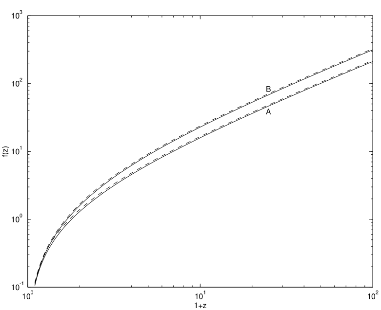
FIG. 1.: Comparison between the luminosity distance, parametrized by $f(z)=H_{0}d_{L}(z)/c$, calculated in two distinct ways. In case I (dashed line) we assume a background universe with cosmological parameters $\Omega^{0}_{\Lambda}$, $\Omega^{0}_{m}$ and ${\cal H}_{0}$ and a perturbation in the vacuum energy density parametrised by $\Delta\Omega^{0}_{\Lambda}$. In case II (solid line) we assume that the cosmological parameters are $\Omega_{m}^{\rm eff}$, $\Omega_{\Lambda}^{\rm eff}$ and ${\cal H}+\Delta{\cal H}$ with no perturbation. Model A has $\Omega^{0}_{m}=1$, $\Omega^{0}_{\Lambda}=0$ and $\Delta\Omega^{0}_{\Lambda}=0.5$ while model B has $\Omega^{0}_{m}=0.3$, $\Omega^{0}_{\Lambda}=0.7$ and $\Delta\Omega^{0}_{\Lambda}=0.2$.

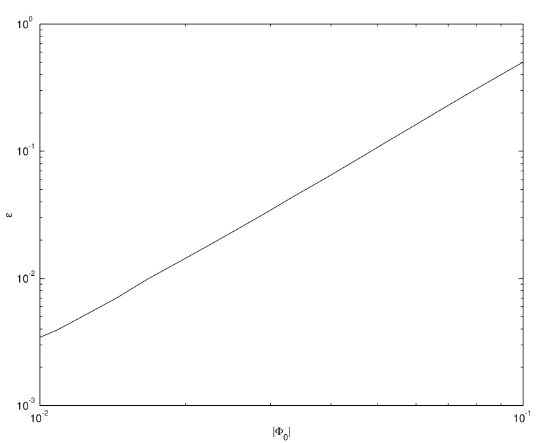
FIG. 2.: Dependence the relative agreement between the two methods for calculating the luminosity distance,$\epsilon$, on the value of $|\Phi_{0}|$ for model $B$ (here we took $\Delta\Omega_{\Lambda}>0$). We see that $\epsilon$ is nearly proportional to $|\Phi_{0}|^{2}$, as expected.

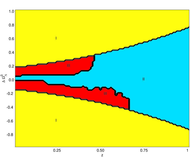
FIG. 3.: The $95\%$ confidence allowed region (region II) in the $z_{*}$ versus $\Delta\Omega^{0}_{\Lambda}$ plane. Region I is excluded since our linear perturbation theory approach does not hold there, while Region III is excluded by the supernovae data. Note the asymmetry between the two observationally excluded regions.

- [1] K.K.S. Wu, O. Lahav and M.J. Rees, astro-ph/9804062 (1998).
- [2] O. Lahav, astro-ph/0001061 (2000).
- [3] T. Kollatt and O. Lahav, astro-ph/0008041 (2000).
- [4] C. A. Clarkson and R. K. Barrett, Class. Quant. Grav. 16, 3781 (1999); R. K. Barrett and C. A. Clarkson, Class. Quant. Grav. 17, 5047 (2000).
- [5] P. P. Avelino, J. P. M de Carvalho and C. J. A. P. Martins, Phys. Lett. B501 257 (2000).
- [6] P. P. Avelino and C. J. A. P. Martins, Phys. Rev. D62, 103510 (2000).
- [7] P. P. Avelino, J. P. M de Carvalho, C. J. A. P. Martins and J. C. R. E. Oliveira, astro-ph/0004227.
- [8] I. Maor, R. Burstein and P. J. Steinhardt, Phys. Rev. Lett. 86, 6 (2001).
- [9] Y. Wang and P. M. Garnavich, Ap. J. 552, 445 (2001).
- [10] M. Tegmark, astro-ph/0101354.
- [11] A. G. Riess et al., Astron. J. 116, 1009 (1998).
- [12] P. M. Garnavich et al., Ap. J. Lett. 493, L53 (1998).
- [13] S. Perlmutter et al., Ap. J. 517, 465 (1999).
- [14] G. Starkman, M. Trodden and T. Vachaspati, Phys. Rev. Lett. 83, 1510 (1999).
- [15] C.J.A.P. Martins and E.P.S. Shellard, Phys. Rev. D53, 575 (1996).
- [16] C.J.A.P. Martins and E.P.S. Shellard, Phys. Rev. D54 2535 (1996).
- [17] C.J.A.P. Martins and E.P.S. Shellard, hep-ph/0003298 (2000).
- [18] P. P. Avelino, A. Canavezes, J. P. M de Carvalho and C. J. A. P. Martins, in preparation.
- [19] V.F. Mukhanov, H.A. Feldman and R.H. Brandenberger, Phys. Rep. 215, 203 (1992).