Abstract

We present the results from the correlation analysis of two galactic redshift surveys, the extended CfA2+SSRS2 and the slice centered on $\delta=-12^{\circ}$ of Las Campanas. Furthermore, we evaluate the likelihood confidence regions for the CDM model and for the fractal model parameters. Our results indicate that, although the CDM model is in good agreement with the data, the fractal description cannot be ruled out, because of its intrinsic high variance.

The availability in the late years of deeper and more accurate redshift surveys allows us not only to better estimate the statistical properties of the galaxy distribution, but also the parameters of the theoretical models. Here we compare the real data with two models that represent two opposite visions of the luminous matter distribution. On one hand the CDM model and its variants state the homogeneity of the galaxy distribution at a scale of order of tens of Mpc (Davis 1997; Cappi et al. 1998); on the other hand the fractal geometrical description of the Universe (Pietronero et al. 1997), assumes that it is completely inhomogeneus at all scales.

To test if a particle distribution has fractal properties, we define the statistical estimator of the correlation function $g(r)=1+\xi(r)$, where $\xi(r)$ is the standard correlation function: if the distribution is fractal with dimension $D$, $g(r)$ decreases as $r^{3-D}$, otherwise it flattens. The correlation $g(r)$ has the further advantage that its estimation in finite volume is simply proportional to its universal value (Amendola 1998).

The applied statistical method is based on the use of the integrated correlation function $\widehat{g}(r)=\int g(r)d^{3}r$ because the differential quantity $g$ is very noisy if it is calculated in low density samples as in Las Campanas (LCRS - Schectman et al. 1996). As usual, we use volume limited (VL) samples to avoid the corrections due to the selection function and the possible dependence on luminosity of the clustering amplitude; we estimate the count cell volumes using Monte Carlo and we ensure that the cell boundaries are completely internal to the survey geometry (Pietronero et al. 1997). The last condition puts a constraint on the value of $R_{M}$, the maximum scale reached via this method, for it depends on the shape of the survey slice, i.e. on its depth $d$ and its minimum angular opening $\theta$. In the case of very narrow slice, as the one of LCRS ($\Delta\delta=1.5^{\circ}$), and if we use spherical cells, $R_{M}$ reaches a few Mpc, while it is crucial to extend the analysis up to scales greater than 50 Mpc/$h$ in order to distinguish between the two competing models. To increase $R_{M}$ we use count cells with the same shape as the survey slice, i.e. same $\theta$ and variable $d$ (radial cells - Amendola & Palladino 1999). In this way we reach deeper scales than the spherical window; for example, in the case of LCRS, we obtain $R_{M}\approx 200$ Mpc/$h$.

We apply the method to seven VL samples, four extracted from the slice centered on $\delta=-12^{\circ}$ of LCRS and three from the extended CfA2+SSRS2 (da Costa et al. 1995). In Tab. I we summarize the characteristic numbers of the samples.

To estimate the variance of $\widehat{g}(r)$ let us make two assumption: the 3-point correlation function is given by the scaling relation $\varsigma_{ijk}=Q(\xi_{ij}\xi_{jk}+\xi_{ij}\xi_{ik}+\xi_{ik}\xi_{jk})$, where we put $Q=1$; $\xi_{ij}$ can be approximated by a power law. So it is possible to demonstrate that the following relation holds (Amendola 1998):

$$\sigma_{\widehat{g}}^{2}=N_{c}^{-1}\left[N_{0}^{-1}\left(1+\widehat{\xi}\right)+\sigma^{2}\left(1+2\widehat{\xi}\right)\right],$$ (1)

where $N_{c}$ is the number of independent cells and $N_{0}$ is the number of galaxies contained on average in the cells.

The expression $P(k)=A\,k\,T^{2}\left(\Gamma,k\right)\,G\left(\Omega_{m},\Omega_{\Lambda},\sigma_{8},\sigma_{v}\right)$ is the power spectrum in a CDM flat universe, where $T\left(\Gamma,k\right)$ is the transfer function of Bardeen et al. (1986), $G$ includes the redshift and nonlinear corrections (Kaiser 1987; Peacock & Dodds, 1996), $\sigma_{v}$ is the line-of-sight velocity dispersion and the subscripts $\Lambda$ and $m$ refer to cosmological constant and total matter, respectively. For the fractal model, the usual integrated correlation function with dimension $D$ and normalization $r_{0}$ is given by $\widehat{\xi}(r)=\left(r/r_{0}\right)^{D-3}-1$. Using these quantities it is possible to evaluate Eq. 1, remembering that $\xi(r)$ is the Fourier transform of $P(k)$ and $\widehat{\xi}(r)$ its volume integral. Notice that in the relation $\sigma^{2}=\left(2\pi^{2}\right)^{-1}\int P\left(k\right)W_{c}\left(k\right)k^{2}dk$ the window $W_{c}\equiv W^{2}$ only if it is spherical, otherwise it has to be calculated numerically.

Finally we perform the likelihood analysis including the free parameters of the model both in the mean and in the variance. For CDM these are the shape factor $\Gamma$ and the galaxy normalization $\sigma_{8}$, where we have fixed $\sigma_{v}=300$ km sec^-1, $\Omega_{m}=0.4$ and $\Omega_{\Lambda}=0.6$; for the fractal model the parameter is $D$ while $r_{0}$ is fixed to be equal to the maximum depth with respect all the samples, i.e. 437 Mpc/$h$. The results of the parameters estimation are given in Tab. I.

Las Campanas							CfA2+SSRS2
VL	$\Delta R$	$N_{gal}$	$\langle M_{S}\rangle$	$\Gamma$	$\sigma_{8}$	$D$	VL	$R$	$N_{gal}$	$M_{lim}$	$\Gamma$	$\sigma_{8}$	$D$
lc410	130	510	$-21.3$	0.2	0.9	2.3	cs19	80	840	$-19.0$	1.0	1.7	2.2
lc330	140	840	$-20.8$	0.1	0.9	2.4	cs20	125	492	$-20.0$	0.2	0.7	2.8
lc297	150	818	$-20.4$	0.2	0.9	2.4	cs205	160	212	$-20.5$	0.1	1.3	2.6
lc437	213	492	$-21.3$	0.2	0.8	2.5

TABLE I
: VL samples and Likelihood results - LCRS has $\Delta\alpha\approx 80^{\circ}$ and $\Delta\delta=1.5^{\circ}$ and because it has two limiting magnitudes, each VL has two cuts in distance, so $\Delta R=R_{2}-R_{1}$. We cut CfA2+SSRS2 to have a regular slice with $\Delta\alpha\approx 80^{\circ}$ and $\Delta\delta\approx 45^{\circ}$.

Fig. 1.: - $\widehat{g}(r)$ in all the seven VL analyzed with the errors expected in a CDM and in a fractal model (dotted lines). The parameters used to estimate the error bars are given in Tab. II

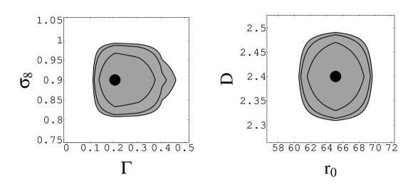
Fig. 2.: - Here are the contour plots (68, 90, 95%) of the product of the likelihood functions for each VL of LCRS; on the left there is the CDM model, on the right the fractal one.

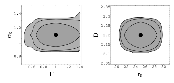
Fig. 3.: - The contour plots (68, 90, 95%) of the VL cs19 of CFA2+SSRS2; on the left there is the CDM model, on the right the fractal one.

As we can see in Fig. 1 the scales we reach are the largest ever reached in $\widehat{g}(r)$ statistics. In Fig. 2, we have shown the contour plots of the product of the likelihood functions of each VL of LCRS, because the estimated parameters are similar in all of them. Our results for LCRS are: $0.12\raise-2.0pt\hbox{\hbox to0.0pt{\hbox{$\sim$}\hss}\raise 5.0pt\hbox{$<$}\ }\Gamma\raise-2.0pt\hbox{\hbox to0.0pt{\hbox{$\sim$}\hss}\raise 5.0pt\hbox{$<$}\ }0.46$, $0.81\raise-2.0pt\hbox{\hbox to0.0pt{\hbox{$\sim$}\hss}\raise 5.0pt\hbox{$<$}\ }\sigma_{8}\raise-2.0pt\hbox{\hbox to0.0pt{\hbox{$\sim$}\hss}\raise 5.0pt\hbox{$<$}\ }0.99$ for CDM; $2.31\raise-2.0pt\hbox{\hbox to0.0pt{\hbox{$\sim$}\hss}\raise 5.0pt\hbox{$<$}\ }D\raise-2.0pt\hbox{\hbox to0.0pt{\hbox{$\sim$}\hss}\raise 5.0pt\hbox{$<$}\ }2.49$ for fractal. The estimated parameters of CfA2+SSSRS2 are different from one VL to the other (see Tab. II for details) so we do not evaluate the likelihood function product; we show as an example the contour plot of cs19 (Fig. 3). Our conclusions are that $\Gamma\simeq 0.2$ in samples that have around the same absolute magnitude; remembering that in the CDM model $\Gamma=\Omega_{m}h$, this agrees with $\Omega_{m}=0.4$ and $h=0.6\div 0.7$. Furthermore, we cannot yet reject the fractal model due to its intrinsic high variance (Fig. 1); this shows that it is necessary to check the validity of a model including its full variance in the likelihood.

We acknowledge financial support by the Ministry of University and of Scientific and Technical Research.

References

- 1 Amendola, L.: 1998, in Proc. IX Brazilian School of Gravitation and Cosmology, M. Novello ed., Editions Frontières, Paris
- 2 Amendola, L., Palladino, E.: 1999, Astrophys. J. Lett. 514, L1
- 3
- 4 Bardeen, J.M. at al.: 1986, Astrophys. J. 304, 15
- 5
- 6 Cappi, A. et al.: 1998, Astron. Astrophys. 335, 779
- 7
- 8 da Costa, L.N. et al.: 1995, Astrophys. J. Lett. 437, L1
- 9
- 10 Davis, M.: 1997, in Critical Dialogues in Cosmology, N. Turok ed., World Scientific, Singapore, p. 13.
- 11
- 12 Guzzo, L.: 1997, New Astron., 2, 517.
- 13
- 14 Kaiser, N.: 1987, Mon. Not. R. Astr. Soc. 227, 1
- 15
- 16 Peacock, J.A., Dodds S.J.: 1996, Mon. Not. R. Astr. Soc. 280, 19
- 17
- 18 Pietronero, L., Montuori M., Sylos Labini, F.: 1997, in Critical Dialogues in Cosmology, N. Turok ed., World Scientific, Singapore, p. 24.
- 19
- 20 Schectman, S. et al.: 1996, Astrophys. J. 470, 172
- 21