Clusters in the Precision Cosmology Era

Abstract

Over the coming decade, the observational samples available for studies of cluster abundance evolution will increase from tens to hundreds, or possibly to thousands, of clusters. Here we assess the power of future surveys to determine cosmological parameters. We quantify the statistical differences among cosmologies, including the effects of the cosmic equation of state parameter $w$, in mock cluster catalogs simulating a 12 deg² Sunyaev-Zel’dovich Effect (SZE) survey and a deep 10⁴ deg² X–ray survey. The constraints from clusters are complementary to those from studies of high–redshift Supernovae (SNe), CMB anisotropies, or counts of high–redshift galaxies. Our results indicate that a statistical uncertainty of a few percent on both $\Omega_{m}$ and $w$ can be reached when cluster surveys are used in combination with any of these other datasets.

Introduction

Because of their relative simplicity, galaxy clusters provide a uniquely useful probe of the fundamental cosmological parameters. The formation of the large–scale dark matter potential wells of clusters is likely independent of complex gas dynamical processes, star formation, and feedback, and involve only gravitational physics. The observed abundance of nearby clusters implies robust constraints on the amplitude $\sigma_{8}$ of the power spectrum on cluster scales to an accuracy of $\sim 25\%$ white93 ; viana96 . In addition, the redshift–evolution of the observed cluster abundance constrains the matter density $\Omega_{0}$ bahcall98 ; blanchard98 ; viana99 .

In order to be useful for these cosmological studies, the masses of galaxy clusters have to be known. Existing studies utilized the presently available tens of clusters with mass estimates gioia90 ; vikhlinin98 , and as a result, were limited in their scope. The present samples, however, will likely soon be replaced by catalogs of thousands of intermediate redshift and hundreds of high redshift ($z>1$) clusters. At a minimum, the analysis of the European Space Agency X–ray Multi–mirror Mission (XMM) archive for serendipitously detected clusters will yield hundreds, and perhaps thousands of new clusters with temperature measurements romer00 . Dedicated X–ray and SZE surveys could likely surpass the XMM sample in areal coverage, number of detected clusters or redshift depth.

The imminent improvement of distant cluster data motivates us to estimate the cosmological power of future surveys. In particular, we study the constraints provided by a 12 deg² SZE survey carlstrom99 , or by a deep 10⁴ deg² X–ray survey. Our primary goals are (1) to quantify the accuracy to which various cosmological models can be distinguished from a standard $\Lambda$ Cold Dark Matter ($\Lambda$CDM) cosmology; and (2) to contrast constraints from clusters to those available from CMB anisotropy measurements, from high–redshift SNe, or from high–redshift galaxy counts schmidt98 ; perlmutter99 ; newman99 .

The galaxy cluster abundance provides a natural test of models that include a dark energy component with an equation of state parameter $w\equiv p/\rho\neq-1$ turner97 ; caldwell98 ; huterer00 . The value of $w$ directly affects the linear growth of fluctuations, and the angular diameter distance (and hence the SZE decrement and the X–ray luminosity) to individual clusters. We restrict our analysis to a flat universe, and focus on the following four parameters: the matter density $\Omega_{m}$; the equation of state parameter $w$ (assumed to be constant); the Hubble constant $h\equiv H_{0}/100~{}{\rm km~{}s^{-1}~{}Mpc^{-1}}$’ and the amplitude of the power spectrum on $8h^{-1}$Mpc scales, $\sigma_{8}$. A broader range of parameters, including open/closed universes, and evolving $w(z)$, will be examined in future work holder01 . Details of the study described here can be found in haiman01 .

Modeling Details

General Approach

To quantify the power of a future cluster survey to distinguish cosmologies, we utilize the following approach:

1. We pick a fiducial cosmological ($\Lambda$CDM) model, with the parameters $(\Omega_{\Lambda},\Omega_{\rm m},h,\sigma_{8},n)=(0.7,0.3,0.65,0.9,1)$, based on present large scale structure data bahcall99 . We assume this model describes the “real” universe.

2. In the fiducial model, we compute the abundance of clusters $dN_{\rm fid}/dz$ as a function of redshift in a specific (SZE or X–ray) survey. This simulates the dataset that will be available in the future for cosmological tests.

3. We vary parameters of our model, and recompute the cluster abundance $dN_{\rm test}/dz$ as a function of redshift in this new “test” cosmology. In each test cosmology, we set the value of $\sigma_{8}$ by requiring the local cluster abundance at redshift $z\approx 0$ to match the value in the fiducial cosmology.

4. We compute the likelihood of observing the redshift distribution $dN_{\rm fid}/dz$ if the true distribution were $dN_{\rm test}/dz$. We utilize both the normalization and shape of the distributions, by combining the standard Poisson and Kolmogorov–Smirnov tests.

5. We repeat steps 3 and 4 for a wide range of values of $w$, $\Omega_{m}$, and $h$.

Predicting Cluster Abundance and Evolution

The fundamental ingredient of this approach is the cluster abundance, given a cosmology and the parameters of a survey. In this study, we utilize the “universal” halo mass function found in a series of recent large–scale cosmological simulations jenkins00 . Following these simulations, we assume that the comoving number density of clusters at redshift $z$ with mass $M$ is given by

$$\frac{dn}{dM}(z,M)=0.315\frac{\rho_{0}}{M}\frac{1}{\sigma_{M}}\frac{d\sigma_{M}}{dM}\exp\left[-\left|0.61-\log(D_{z}\sigma_{M})\right|^{3.8}\right],$$ (1)

where $\sigma_{M}$ is the present day r.m.s. density fluctuation on mass–scale $M$eisenstein98 , $D_{z}$ is the linear growth function, and $\rho_{0}$ is the present–day mass density. The directly observable quantity is the number of clusters with mass above $M_{\rm min}$ at redshift $z\pm dz/2$ in a solid angle $d\Omega$:

$$\frac{dN}{dzd\Omega}\left(z\right)=\left[\frac{dV}{dzd\Omega}\left(z\right)\int_{M_{\rm min}(z)}^{\infty}dM\frac{dn}{dM}\right]$$ (2)

where $dV/dzd\Omega$ is the cosmological volume element, and $M_{\rm min}(z)$ is the limiting mass of the survey, as discussed below. Equations 1 and 2 reveal that the cluster abundance depends on cosmology through several quantities: (1) the growth function $D_{z}$; (2) the volume element $dV/dzd\Omega$; (3) the power spectrum $\sigma_{M}$; (4) the mass density $\rho_{0}$; and (5) the survey mass threshold $M_{\rm min}$. The first four of these dependencies are well–determined, once the parameters of the cosmological model and the power spectrum are specified (in particular, note that the abundance is exponentially sensitive to the growth function). The scaling of the limiting mass with cosmology depends on the specific survey.

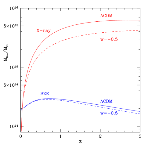
Figure 1: Limiting cluster virial masses for detection in a 10⁴ deg² X–ray survey (upper pair of curves) and in a 12 deg² SZE survey (lower pair of curves). The solid curves show the mass limit in our fiducial flat $\Lambda$CDM model, with $w=-1$, $\Omega_{m}=0.3$, and $h=0.65$, and the dotted curves show the masses in the same model except with $w=-0.5$.

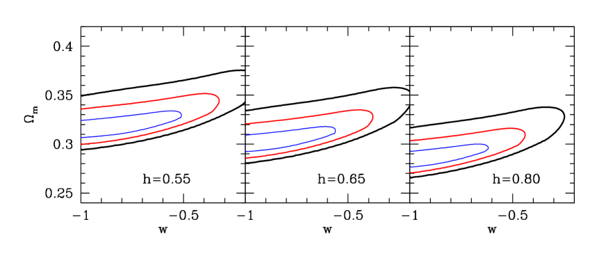
Figure 2: Contours of 1, 2, and 3$\sigma$ likelihood for different models when they are compared to a fiducial flat $\Lambda$CDM model with $\Omega_{m}=0.3$ and $h=0.65$, using the SZE survey. The three panels show three different cross–sections of constant total probability at fixed values of $h$ (0.55,0.65, and 0.80) in the investigated 3–dimensional $\Omega_{m},w,h$ parameter space.

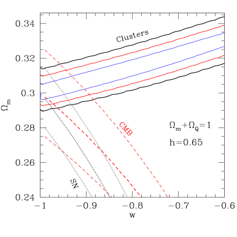
Figure 3: Likelihood contours for a fixed $h=0.65$ in the X–ray survey. Also shown are combinations of $w$ and $\Omega_{m}$ that keep the spherical harmonic index $\ell$ of the first Doppler peak in the CMB anisotropy data constant to within $\pm 1\%$ (dashed lines); and combinations that keep the luminosity distance to redshift $z=1$ constant to the same accuracy.

Cluster Surveys

In this study, we examine two specific surveys, in which clusters are detected through either their SZ decrements, or X–ray fluxes. In practice, the only survey details we utilize in our analyses are the virial mass of the least massive, detectable cluster (as a function of redshift and cosmological parameters), and the solid angle of the survey. The SZE survey we consider is that proposed by J. Carlstrom and collaborators carlstrom99 . This interferometric survey will detect clusters more massive than $\sim 2\times 10^{14}M_{\odot}$, nearly independent of their redshift, and will cover an area of 12 deg² in a year. The relatively small solid angle of the survey will allow cluster redshifts to be determined by deep optical and near infrared followup observations. The X–ray survey we consider is similar to a proposed Small Explorer mission, called the Cosmology Explorer, spear-headed by G. Ricker and D. Lamb. The survey depth is $3.6\times 10^{6}$ cm²s at 1.5 keV, and the coverage is 10⁴ deg² (approximately half the available unobscured sky). We focus on clusters which produce 500 detected source counts in the 0.5:6.0 keV band, sufficient to reliably estimate the emission weighted mean temperature. The X–ray survey could be combined with the Sloan Digital Sky Survey (SDSS) to obtain redshifts for the clusters.

The most important aspect of both surveys is the limiting halo mass $M_{\rm min}(z,\Omega_{m},w,h)$, and its dependence on redshift and cosmological parameters. For an interferometric SZE survey, the relevant observable is the cluster visibility $V$, which is proportional to the total SZE flux decrement. The detection limit as a function of redshift and cosmology for this survey has been studied using mock observations of simulated galaxy clusters holder00 . In the X–ray survey, $M_{\rm min}$ follows from the cluster X–ray luminosity – virial mass relation bryan98 . Illustrative examples of the mass limits in both surveys are shown in Figure 1, both for $\Lambda$CDM and for a $w=-0.5$ universe. The SZE mass limit is nearly independent of redshift, and changes little with cosmology. As a result, the cluster sample can extend to $z\approx 3$. In comparison, the X–ray mass limit is a stronger function of $w$, and it rises rapidly with redshift. For the X–ray survey considered here the number of detected clusters beyond $z\approx 1$ is negligible. The total number of clusters in the SZE survey is $\sim 200$, while in the X–ray survey, it is $\sim 2,000$.

Results and Conclusions

Our results are summarized by the likelihood contours in the $\Omega_{m}-w$ plane, shown in Figures 2 and 3 for the SZE and X–ray surveys, respectively. Figure 2 shows three different cross–sections of constant total probability in the SZE survey, at fixed values of $h$ (0.55,0.65, and 0.80) in the investigated 3–dimensional $\Omega_{m},w,h$ parameter space. These diagrams demonstrate that the constraints on $\Omega_{m}$ are at the $\sim 10\%$ level, while $w$ remains essentially unconstrained ($w\;\hbox to0.0pt{\lower 2.5pt\hbox{$\sim$}\hss}\raise 1.5pt\hbox{$<$}\;-0.2$). Nevertheless, the narrowness of the contours in Figure 2 implies that the SZE survey can yield accurate constraints on $w$ if combined with other data. We find that the differences among cosmologies in the SZE survey are driven nearly entirely by the growth function $D_{z}$. This results from the cluster sample extending to high redshifts ($z>1$), where the growth functions in different cosmologies diverge rapidly. This makes the SZE sample especially useful. For comparison, galaxy counts at $z\sim 1$ probe mostly the cosmological volume, and constitute and independent test from clusters newman99 . Note that our constraints scale weakly with $h$: this arises from the weak dependence of the power spectrum on $h$.

Figure 3 shows constraints in the X–ray survey for a fixed $h=0.65$. The increased number of clusters translates to significantly narrower contours compared to the SZE survey. The orientation of the contours remains similar, but we find that the cosmological sensitivity arises nearly entirely from the mass limit $M_{\rm min}$. Indeed, the X–ray flux is more sensitive to cosmology than the SZE decrement (cf. Fig. 1), and the X–ray sample extends only out to $z\sim 1$, where the growth functions are less divergent. Also shown in Figure 3 are constraints expected from CMB anisotropies and from high–$z$ SNe. The dashed curves correspond to the CMB constraints (a $\pm 1\%$ determination of the position of the first Doppler peak); the dotted curves to the constraints from SNe (a $\pm 1\%$ determination of the luminosity distance to $z=1$). As these curves show, the constraints from the CMB and SNe data are complementary to the direction of the parameter degeneracy in cluster abundance studies, making the cluster surveys especially valuable.

Our findings suggest that cluster surveys will lead to tight constraints on a combination of $\Omega_{m}$ and $w$, especially valuable because of their high complementarity to constraints from CMB anisotropies, magnitudes of high–$z$ SNe, or counts of high–$z$ galaxies. In combination with either of these data, clusters can determine both $\Omega_{m}$ and $w$ to a few percent accuracy. We have focused primarily on the statistics of cluster surveys: further work is needed to clarify the role of systematic uncertainties, arising from the cosmology–scaling of the mass limits and the the cluster mass function, as well as our neglect of issues such as galaxy formation in the lowest mass clusters.

We thank J. Carlstrom and the COSMEX team for providing access to proposed instrument characteristics. ZH acknowledges support from a Hubble Fellowship.

References

- (1) White, S.D.M., Efstathiou, G., Frenk, C.S., Mon. Not. Roy. Ast. Soc. 262, 1023 (1993).
- (2) Viana, P.T.P. and Liddle, A.R., Mon. Not. Roy. Ast. Soc. 281, 323 (1996).
- (3) Bahcall, N.A. and Fan, X., Ap. J. 504, 1 (1998).
- (4) Blanchard, A. and Bartlett, J.G., Ast. and Astroph. 332, L49 (1998).
- (5) Viana, P.T.P. and Liddle, A.R., Mon. Not. Roy. Ast. Soc. 303, 535 (1999).
- (6) Gioia, I.M., et al., Ap. J. Supp. 72, 567 (1990).
- (7) Vikhlinin, A., et al., Ap. J. 503, 77 (1998).
- (8) Romer, A.K., Viana, P.T.P., Liddle, A.R. and Mann, R.G., Ap. J. 547, 594 (2001).
- (9) Carlstrom, J.E., et al., Physica Scripta T, 148, (2000).
- (10) Schmidt, B.P. et al. Ap. J. 507, 46 (1998).
- (11) Perlmutter, S. et al. Ap. J. 517, 565 (1999).
- (12) Newman, J. A., and Davis, M. Ap. J. 534, L11 (2000).
- (13) Turner, M. S., and White, M., Phys. Rev. D. 56, 4439 (1997).
- (14) Caldwell, R.R., Dave, R. and Steinhardt, P.J., Ast. Space Sci. 261, 303 (1998).
- (15) Huterer, D., and Turner, M. S., Phys. Rev. D. submitted, astro-ph/0012510
- (16) Holder, G.P., Haiman, Z., Mohr, J.J., Turner, M. S., & Carlstrom, J.E., in prep; see also these proceedings.
- (17) Haiman, Z., Mohr, J.J., and Holder, G.P., Ap. J., in press, astro-ph/0002336 (2001).
- (18) Bahcall, N.A., et al., Science 284, 1481 (1999).
- (19) Jenkins, A. et al., Mon. Not. Roy. Ast. Soc. 321, 372 (2001).
- (20) Eisenstein, D.J. and Hu, W. Ap. J. 504, L57 (1998).
- (21) Holder, G.P., et al., Ap. J. 544, 629 (2000).
- (22) Bryan, G.L. and Norman, M.L. Ap. J. 495, 80 (1998).