Abstract

We constrain the spectrum of primordial curvature perturbations by using recent Cosmic Microwave Background (CMB) and Large Scale Structure (LSS) data. Specifically, we consider CMB data from the COBE, Boomerang and Maxima experiments, the real space galaxy power spectrum from the IRAS PSCz survey, and the linear matter power spectrum inferred from Ly$-\alpha$ forest spectra, where we for simplicity assume the absence of appreciable covariances. We study the case of single field slow roll inflationary models, and we extract bounds on the scalar spectral index, $n$, the tensor to scalar ratio, $r$, and the running of the scalar spectral index, $\partial_{{\rm ln}k}$, for various combinations of the observational data. We find that CMB data, when combined with data from Lyman$-\alpha$ forest, place strong constraints on the inflationary parameters. Specifically, we obtain $n\approx 0.9$, $r\raise 1.29167pt\hbox{$\;<$\kern-7.5pt\raise-4.73611pt\hbox{$\sim\;$}}0.3$ and $\partial_{{\rm ln}k}\approx 0$, indicating that big n, big r models (often referred to as hybrid models) are ruled out.

PACS: 98.62.Ra, 98.65.-r, 98.70.Vc, 98.80.Cq

1 Introduction

Inflation is generally believed to provide the initial conditions for the evolution of large scale structure (LSS) and the cosmic microwave background radiation (CMB). The garden of inflation offers a bounty of models, each of which predicts a certain power spectrum of primordial curvature perturbations, ${\cal P}(k)$, a function of the wavenumber $k$. This power spectrum can be Taylor-expanded about some wavenumber $k_{0}$ and truncated after a few terms [1]

$${\rm ln}{\cal P}(k)={\rm ln}{\cal P}(k_{0})+(n-1)\,{\rm ln}\frac{k}{k_{0}}+\left.\frac{1}{2}\frac{d\,n}{d\,{\rm ln}k}\right|_{k_{0}}\,{\rm ln}^{2}\frac{k}{k_{0}}+\cdots$$ (1)

in which the first term is a normalization constant, the second is a power-law approximation, with the case $n=1$ corresponding to a scale invariant Harrison-Zel’dovich spectrum, and the third term is the running of the spectral index.

An important class of models is given by single field slow roll (SR) inflationary models, which can be treated perturbatively. The properties of SR models are well known (see e.g. ref. [2] for review and a list of references), and we will here classify the different models by the 3 parameters $(n,r,\partial_{{\rm ln}k})$, where $n\equiv d\ln{\cal P}/d{\rm ln}k|_{k=k_{0}}+1$ is the scalar spectral index at the pivot scale $k_{0}$, the parameter $r$ is the tensor to scalar perturbation ratio at the quadrupole scale, and $\partial_{{\rm ln}k}\equiv dn/d{\rm ln}k|_{k=k_{0}}$. The reason for using these 3 variables instead of the normal SR parameters $(\epsilon,\eta,\xi^{2})$ (defined in the appendix) is simply that the former 3 variables are more closely related to what is measured from observations.

In SR models the tensor spectral index and its derivative can be expressed [2, 3]

$$n_{T}=-\frac{r}{\kappa}\,\,\,\,\,{\rm and}\,\,\,\,\,\frac{d\,n_{T}}{d\,{\rm ln}k}=\frac{r}{\kappa}\left[\left(n-1\right)+\frac{r}{\kappa}\right]~{}.$$ (2)

The factor $\kappa$ in the above equations depends on the model, and in particular is different for different $\Omega_{\Lambda}$ [4]. In our analysis we use the parametrisation from ref. [5], which for the models considered here means $5\leq\kappa\leq 7$.

The different SR models are traditionally [6] categorised into 3 main groups according to the relationship between the first and second derivative of the inflaton potential, and they are distributed in $(n,r)$ and $(n,\partial_{{\rm ln}k})$ space as in Fig. 1 (see details in the appendix or in ref. [7]), where the dashed lines on the borders between the different models are the two attractors found in ref. [8], $r=0$ and $r=-\kappa(n-1)$. For large values of $n-1$ and $r$, SR models “naturally” predict sizeable deviations from a power law approximation (i.e. $\partial_{{\rm ln}k}\neq 0$), so when comparing to observations it is important to include the third parameter $\partial_{{\rm ln}k}$, in addition to the parameters $n$ and $r$ commonly considered.

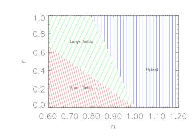
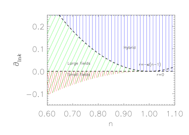
Figure 1: The various slow-roll models in $(n,r)$ and $(n,\partial_{{\rm ln}k})$ space. The dashed lines are the two attractors (here we have used $\kappa=5$ which is a typical value for a flat universe with a large cosmological constant). The figure $(n,\partial_{{\rm ln}k})$ is for $\xi^{2}=0$. The hatched regions move up and down by inclusion of the third derivative, $\xi^{2}\neq 0$ (see Eq. 10 in the appendix).

The purpose of this paper is to ascertain what constraints currently available observational data can place on the parameters $(n,\partial_{{\rm ln}k},r)$ of SR inflation. Of course the universe could lie outside the hatched regions of Fig. 1, indicating that one should look beyond SR inflation; but it seems reasonable to explore the simplest models in the first instance. In ref. [7], CMB data were used to put bounds on inflationary parameters, and indications were found towards a negative bend of the primordial power spectrum ($\partial_{{\rm ln}k}\leq 0$). However, the scales probed by CMB are limited, and the constraint on $\partial_{{\rm ln}k}$ was weak.

In the present paper we extend the analysis of [7] by including information not only from the CMB, but also from the linear galaxy power spectrum measured from the IRAS Point Source Catalogue Redshift (PSCz) survey [9], and from the linear matter power spectrum inferred from the Ly$-\alpha$ forest in quasar spectra [10]. Even though it is not completely clear that the correlations in the 3d matter power spectrum are negligible, we treat them as such for simplicity. The size of and effect from such covariances might be essential, and should be considered more carefully in a future investigation. As we will show, these data, probing different ranges of scales, yield much tighter constraints on the inflationary parameters than CMB data alone.

2 The data

Recently observational data on both the CMB and LSS have improved dramatically. The balloon-borne experiments Boomerang [15] and MAXIMA [16] have determined the CMB angular power spectrum beyond the first acoustic peak, whose position near $l\sim 200$ indicates a flat universe, hence seemingly confirming the inflationary paradigm. The two experiments, together with COBE-DMR [18], provide a high signal-to-noise determination of the CMB power spectrum for $2<l\raise 1.29167pt\hbox{$\;<$\kern-7.5pt\raise-4.73611pt\hbox{$\sim\;$}}800$, thus testing the structure formation paradigm on scales roughly of the order $k\raise 1.29167pt\hbox{$\;<$\kern-7.5pt\raise-4.73611pt\hbox{$\sim\;$}}0.1$ $h$ Mpc^-1.

LSS data, probing smaller scales, provide complementary information. In this paper we consider the real space galaxy power spectrum from IRAS Point Source Catalogue Redshift (PSCz) survey [19] which probes scales in the range $k=0.01-300$ $h$ Mpc^-1 [9, 17]. In order to avoid problems with the interpretation of non-linear effects, we use data only at scales $k\leq 0.3$ $h$ Mpc^-1.

Further, we consider the information on the linear matter spectrum at redshift $z\sim 3$ which can be inferred from the Ly-$\alpha$ forest in quasar spectra. The fact that the nonlinear scale is smaller at higher redshift makes it possible to probe the linear power spectrum to smaller scales ($k\sim 0.2-5$ $h$ Mpc^-1) than are accessible to galaxy surveys at low redshift. In this paper we use a recent determination [10] of the linear matter power spectrum from the Lyman-$\alpha$ forest at redshift $z=2.72$, based on a large sample of Keck HIRES and Keck LRIS quasar spectra. To convert the measured power spectrum of Ly-$\alpha$ flux into the matter power spectrum, [10] apply a correction factor obtained from $N$-body computer simulations. To allow for possible systematic uncertainty [20] in this correction factor, we will repeat the analysis excluding the data at the smallest scales.

2.1 Data analysis

In order to investigate how the CMB, PSCz and Ly-$\alpha$ data constrain the SR parameter space $(n,r,\partial_{{\rm ln}k})$, we performed a likelihood analysis of the data sets from COBE [18], Boomerang [15] and MAXIMA [16], together with the decorrelated linear power spectrum of PSCz galaxies for $k\leq 0.3$ $h$ Mpc^-1 [9, 17], and the Ly-$\alpha$ data from Table 4 of ref. [10]. The likelihood function is

$${\cal L}\propto\exp(-\chi^{2}/2),$$ (3)

where

$$\chi^{2}=\chi^{2}_{\rm CMB}+\chi^{2}_{\rm PSCz}+\chi^{2}_{{\rm Ly-}\alpha}.$$ (4)

For the CMB data

$$\chi^{2}_{\rm CMB}=\sum_{i}\frac{(C_{l,i}(\theta)-C_{l,i})^{2}}{\sigma^{2}(C_{l,i})},$$ (5)

while for PSCz and Ly-$\alpha$ data

$$\chi^{2}_{{\rm PSCz,Ly-}\alpha}=\sum_{i}\frac{(P_{k,i}(\theta)-P_{k,i})^{2}}{\sigma^{2}(P_{k,i})},$$ (6)

the sum being taken over published values of band-powers $C_{l,i}$ and $P_{k,i}$. The quantity $\theta$ is a vector of cosmological parameters, taken here to be

$$\theta=\{\Omega_{m},\Omega_{\Lambda},\Omega_{b},H_{0},\tau,Q,n,r,\partial_{{\rm ln}k}\}~{}.$$ (7)

The parameters are: the matter density $\Omega_{m}$; the baryon density $\Omega_{b}$; the Hubble parameter $H_{0}$; the optical depth $\tau$ to reionization; the normalizations $Q_{\rm CMB}$, $Q_{\rm PSCz}$, and $Q_{{\rm Ly-}\alpha}$ of the CMB, LSS, and Ly-$\alpha$ power spectra; and the inflationary parameters $n,r,\partial_{{\rm ln}k}$. We have assumed that the universe is flat, $\Omega_{\Lambda}=1-\Omega_{m}$, as predicted by standard inflationary models. For all the figures we marginalize over all other parameters. We consider only two values for the baryon density, $\Omega_{b}h^{2}=0.019$ and $0.030$, however, as we will see, the results are very similar in those two cases, suggesting that the results will be similar if allowing $\Omega_{b}h^{2}$ as a free parameter.

The CMB, LSS, and Ly-$\alpha$ data are all subject to uncertainties in their overall normalizations. The CMB groups quote estimated calibration errors for their experiments, which we account for by allowing the data points to shift up or down, by 10% for Boomerang [15], and by 4% for MAXIMA [16]. Because of uncertainty in the linear galaxy-to-mass bias for PSCz galaxies [17], we conservatively treat the normalization $Q_{\rm PSCz}$ as an unconstrained parameter. Ref. [10] quotes uncertainties in the overall normalization of the matter power spectrum inferred from the Ly-$\alpha$ forest, but these uncertainties are based on simulations with $\partial_{{\rm ln}k}=0$, so to avoid possible bias we again conservatively treat the normalization $Q_{{\rm Ly}\alpha}$ as an unconstrained parameter.

For simplicity all data points have been treated as uncorrelated in the likelihood functions, eqs. (5,6). For the CMB data, correlations between estimates $C_{l,i}$ of angular power at different harmonics $l$ are induced by finite sky coverage, but in practice the CMB teams quote band-powers at sufficiently well-separated bands of $l$ that the correlations are probably small. For the PSCz data, the published band-powers are explicitly decorrelated. For the Ly-$\alpha$ data, the covariances between estimates of the flux power spectrum are small, according to Fig. 12 of [10], and this may translate into small statistical covariances in the inferred matter power spectrum. As mentioned earlier, it is not completely clear how good this translation from flux power to matter power is, and we leave this question for future investigation.

We have chosen the pivot scale in Eq. (1) as $k_{0}=0.05\,{\rm Mpc}^{-1}$. This choice is made for convenience, since $k_{0}=0.05\,{\rm Mpc}^{-1}$ is the scale at which wave-numbers are normalised in the CMBFAST code. Our results are independent of the value of $k_{0}$.

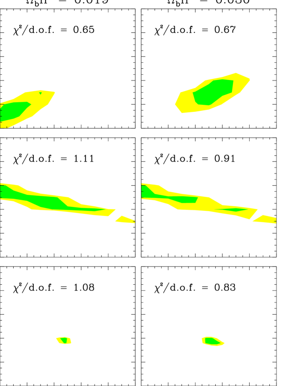
Figure 2: The 1 and 2 $\sigma$ allowed regions for the two slow roll parameters $n$ and $\partial_{{\rm ln}k}$. The left panels assume a BBN prior on $\Omega_{b}h^{2}=0.019$, whereas the right panels are for $\Omega_{b}h^{2}=0.030$, the value which best fits the CMB data. The top row is for CMB data alone, the middle row is for Lyman-$\alpha$ data alone, and the bottom row is for the combined analysis.

2.2 Results

The analysis of the constraints from CMB data was presented in detail in ref. [7] (see also [21]). Here we extend the analysis in [7] by including the reionization optical depth, $\tau$, as a free parameter. This is potentially important since there is a well-known degeneracy between $\tau$ and the scalar spectral index $n$. However, the analysis turns out to prefer models with $\tau\approx 0$, so including $\tau$ leaves the main conclusions of [7] essentially unchanged, as can be seen in the upper panels of Figs. 2 and 3. We recall here the main conclusions from [7]: (1) if we allow the primordial power spectrum to bend, $\partial_{{\rm ln}k}\neq 0$, then CMB data do not constrain the tensor to scalar perturbation ratio $r$; (2) if we assume a BBN prior, $\Omega_{b}h^{2}=0.019$ [24], then CMB data favour a negative bend, $\partial_{{\rm ln}k}<0$, corresponding to a bump-like feature centered at scales $k\sim 0.004\,\rm{Mpc}^{-1}$.

Let us now discuss the information on the inflationary parameters which emerges from PSCz and Ly-$\alpha$ data. The first observation is that PSCz data do not provide relevant constraints in the $(n,\partial_{{\rm ln}k})$ plane. This is easily understood, because the PSCz data at large scales (say $k<0.03\,h\,\rm{Mpc}^{-1}$) have large errors and therefore play little role in the $\chi^{2}$ evaluation. This implies that PSCz data effectively span only one decade in $k$. Considering that the overall normalization of the data is taken as a free parameter, it is evident that one cannot obtain strong constraints from such a small range of scales.

The situation is quite different with Ly-$\alpha$ data, which have small error bars and span almost two decades in $k$. This is shown in Fig. 2, where we present the allowed regions corresponding to 1 and 2 $\sigma$ (we define the $1\sigma$ region as $\chi^{2}\leq\chi^{2}_{\rm min}+2.3$ and the 2$\sigma$ region as $\chi^{2}\leq\chi^{2}_{\rm min}+6.17$) for both $\Omega_{b}h^{2}=0.019$ as suggested by BBN (left column), and $\Omega_{b}h^{2}=0.03$ as suggested by CMB (right column). The top graphs are from CMB data alone, the middle graphs are obtained using Ly-$\alpha$ data alone, and the bottom graphs are from the combined analysis.

It is straightforward to understand how Ly-$\alpha$ data select the allowed regions shown in the middle panels of Fig. 2. At the small scales probed by Ly-$\alpha$ data, the theoretical linear matter power spectrum $P(k)$ is roughly proportional to

$$P(k)\propto\ln^{2}(\alpha k/\Gamma h)\,k^{n^{\prime}-4}$$ (8)

where $\alpha=2.205$, $\Gamma=\Omega_{m}h$ and $k$ is expressed in $\rm{Mpc}^{-1}$ [25]. The parameter $n^{\prime}=d\ln{\cal P}(k_{\alpha})/d\ln k+1$ is the effective spectral index of primordial density perturbation at the scale $k_{\alpha}\approx 3.7(\Omega_{m}h^{2}/0.4)^{1/2}$ Mpc^-1 representative of Ly-$\alpha$ data . On the other hand the Ly-$\alpha$ data, as discussed in [10], are well fitted by a power law, $P(k)\sim k^{\nu}$, with spectral index $\nu=-2.47\pm 0.06$. This means that

$$\frac{d\ln P(k_{\alpha})}{d\ln k}=(n^{\prime}-4)+\frac{2}{\ln(\alpha k_{\alpha}/\Gamma h)}=-2.47\pm 0.06~{}.$$ (9)

If we consider that $\Omega_{b}h^{2}\raise 1.29167pt\hbox{$\;<$\kern-7.5pt\raise-4.73611pt\hbox{$\sim\;$}}\Gamma h\raise 1.29167pt\hbox{$\;<$\kern-7.5pt\raise-4.73611pt\hbox{$\sim\;$}}1$, the previous expression can be directy translated into a bound for the effective spectral index of primordial density perturbations. We obtain $n^{\prime}\sim 0.75-1.1$, which roughly corresponds to what is shown in the middle panels of Fig. 2 for $\partial_{{\rm ln}k}=0$. It is also easy to understand the observed correlation between $n$ and $\partial_{{\rm ln}k}$. The effective spectral index $n^{\prime}$ can be expressed, as a function of $n$ and $\partial_{{\rm ln}k}$, by $n^{\prime}=n+\ln(k_{\alpha}/k_{0})\partial_{{\rm ln}k}$. It is thus evident that the allowed region in the plane $(n,\partial_{{\rm ln}k})$ lies roughly along lines of constant $n^{\prime}$.

It is important to note that the regions constrained by Ly-$\alpha$ data are “orthogonal” to the regions constrained by CMB data. This means that the combined analysis (CMB+Ly-$\alpha$) gives much stronger bounds than any of the two alone. Moreover, since CMB data provide a bound on $\Omega_{m}h^{2}$, the degeneracy between $n^{\prime}$ and $\Gamma h$ in Eq. (9) is removed, and therefore the Ly-$\alpha$ observation of $P(k)\propto k^{-2.47\pm 0.06}$ can be directly translated into a constraint on $n^{\prime}$. This is clearly shown in the lower panels of Fig. 2, from which one obtains the following conclusions: (1) the combined analysis strongly indicates that the bend of the primordial power spectrum is close to zero, being $-0.05<\partial_{{\rm ln}k}<0.02$ at the 2$\sigma$ level; (2) the spectral index $n$ is constrained to be fairly close to $n=0.9$. One notes that the limits obtained do not crucially depend on the assumed values of $\Omega_{b}$, indicating that the inclusion of Lyman-$\alpha$ data avoids the problem with CMB data alone, that different $\Omega_{b}$ extend the allowed range of the spectral index beyond $n\approx 1$ [21]. However, one should note that, due essentially to CMB data, the goodness of the fit is quite sensitive to the assumed value of $\Omega_{b}$, the $\chi^{2}$ being substantially smaller for high $\Omega_{b}$.

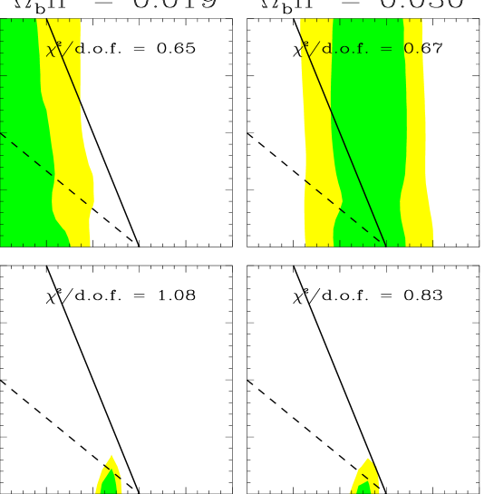
Figure 3: The 1 and 2 $\sigma$ allowed regions in the $(n,r)$ plane. The left panels assume a BBN prior on $\Omega_{b}h^{2}=0.019$, whereas the right panels are for $\Omega_{b}h^{2}=0.030$, the value which best fits the CMB data. The top panels are for CMB data alone, while the bottom panels are for the combined analysis. Hybrid models are to the right of the full line.

In Fig. 3 we present the constraints obtained for the remaining SR parameter $r$. Specifically, we show the 1 and 2 $\sigma$ allowed regions in the $(n,r)$ plane, for both low and high $\Omega_{b}$. The top panels are from CMB data alone, while the bottom ones are from the combined analysis. It is clear that in the combined analysis $r$ is constrained to be smaller than about 0.3 at 2 $\sigma$. This is substantially different from the analysis of CMB data alone, where no constraints on $r$ could be obtained, since a strong bend, e.g. $\partial_{{\rm ln}k}=-0.2$, could allow the tensor component to be big [7]. It is worth noting, that Ly-$\alpha$ data don’t probe $r$ directly; they fix $n$ to be less than 1, and $\partial_{{\rm ln}k}$ close to zero. In this way strong constraint on $r$ can be obtained from CMB data. This result is extremely important when we compare to theoretical models, since different classes of models predict different relationships between the scalar spectral index $n$ and the tensor to scalar ratio $r$ (see Fig. 1). The combined analysis, indicating $n\approx 0.9$ and $r\raise 1.29167pt\hbox{$\;<$\kern-7.5pt\raise-4.73611pt\hbox{$\sim\;$}}0.3$, favours small field models and seems to exclude hybrid models. This is clear from the lower panels of Fig. 3, where the big n, big r (often referred to as hybrid models, to the right of the full line), are excluded at 2$\sigma$. 

An important caveat to this analysis concerns possible systematic uncertainties in the inference of a linear matter power spectrum from the Ly-$\alpha$ data. What [10] measure directly from observations is the power spectrum of transmitted Ly-$\alpha$ flux. The conversion to a linear matter power spectrum involves a fairly large, scale-dependent correction which [10] extract from collisionless computer simulations, with the Ly-$\alpha$ optical depth taken proportional to a certain power of the dark matter density [13]. It has been suggested [20] that the relation between baryonic and dark matter densities could introduce significant uncertainty in the flux-to-mass correction at small scales. Specifically, pressure effects cause the baryonic density $\delta_{b}$ to be smoothed compared to the dark matter density $\delta_{d}$, an effect that can be parametrized as $\delta_{b}({\bf k})=\exp[-(k/k_{f})^{2}]\delta_{d}({\bf k})$, with comoving filter scale $k_{f}\sim 35\,h\,{\rm Mpc}^{-1}$ [14]. The procedure considered by [20] is to treat the filter scale $k_{f}$ as a free parameter constrained only by the shape of the power spectrum of Ly-$\alpha$ flux. However, [10] argue that treating $k_{f}$ as a free parameter is overly pessimistic, and that if $k_{f}$ takes values suggested by hydrodynamic simulations, then the effect on the power spectrum is minor.

To allow for the possibility that the systematic errors are underestimated at small scales, we repeated the analysis neglecting the last 3 data-points from the Ly-$\alpha$ data [10], both for $\partial_{{\rm ln}k}=0$ and for $\partial_{{\rm ln}k}$ free. The upper panels in Fig. 4 show the case where $\partial_{{\rm ln}k}=0$. Here, the results are essentially unchanged by the removal of the data points. However, the lower panels show the full case. Here, the tight constraint on $r$ disappears completely, and the constraint on $n$ is significantly weakened. The reason is that the small scale data points are the most important for constraining $\partial_{{\rm ln}k}$. When these points are removed, $\partial_{{\rm ln}k}$ is not nearly as tightly constrained as before, and as seen for the case where only CMBR data is used, a large $r$ can be compensated by a negative bend of the spectrum.

Thus, the very tight constraint derived above depends on the correctness of the small scale Ly-$\alpha$ data. Therefore, it is highly desirable that a better understanding of the possible systematic errors in determining matter power spectra from Ly-$\alpha$ forest observations is developed.

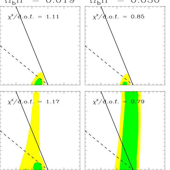
Figure 4: The 1 and 2 $\sigma$ allowed regions in the $(n,r)$ plane. These results are obtained from the combined analysis, neglecting the last 3 data-points from [10]. The left panels assume a BBN prior on $\Omega_{b}h^{2}=0.019$, whereas the right panels are for $\Omega_{b}h^{2}=0.030$, the value which best fits the CMB data. The top panels assume $\partial_{{\rm ln}k}=0$, whereas the lower panels have $\partial_{{\rm ln}k}$ as a free parameter. Hybrid models are to the right of the full line.

Another worry is that the error ellipses for CMB and Ly-$\alpha$ are only marginally overlapping. This might indicate that the two data sets are mutually inconsistent, and that other physical effects should be taken into account. For the Ly-$\alpha$ data one might think of massive neutrinos or warm dark matter, where both would suppress power on small scales, potentially allowing bigger $n$ or bigger positive $\partial_{{\rm ln}k}$.

3 Conclusions

We have considered data from both CMB and LSS to place constraints on the parameters of single field slow roll inflationary models. We have found that, by combining CMB data with the power spectrum inferred from Lyman$-\alpha$ forest, one obtains strong constraints on the inflationary parameters. We obtain $0.8\raise 1.29167pt\hbox{$\;<$\kern-7.5pt\raise-4.73611pt\hbox{$\sim\;$}}n\raise 1.29167pt\hbox{$\;<$\kern-7.5pt\raise-4.73611pt\hbox{$\sim\;$}}1.0$, $r\raise 1.29167pt\hbox{$\;<$\kern-7.5pt\raise-4.73611pt\hbox{$\sim\;$}}0.3$ and $-0.05\raise 1.29167pt\hbox{$\;<$\kern-7.5pt\raise-4.73611pt\hbox{$\sim\;$}}\partial_{{\rm ln}k}\raise 1.29167pt\hbox{$\;<$\kern-7.5pt\raise-4.73611pt\hbox{$\sim\;$}}0.02$ at $2\sigma$ level. In the language of SR this means $\epsilon<0.03$ and $\eta<0.06$, with the best fit model being small fields. This still leaves a large part of the SR parameter space open, but seems to exclude big n, big r models, often referred to as hybrid models. These constraints are much stronger than those from CMB data alone, and arise because the error-ellipse from Ly-$\alpha$ data is almost perpendicular to the error-ellipse from CMB data. Let us repeat, that we in this analysis for simplicity have assumed the absence of appreciable covariances between the reconstructed Ly-$\alpha$ mass powers.

Appendix A Notation

We use the notation: $\eta\equiv\alpha\,\epsilon$, where

$$\epsilon=\frac{M^{2}}{2}\left(\frac{V^{\prime}}{V}\right)^{2}\,\,\,~{},\,\,\,\eta=M^{2}\frac{V^{\prime\prime}}{V}-\frac{M^{2}}{2}\left(\frac{V^{\prime}}{V}\right)^{2}\,\,\,\mbox{and}\,\,\,\xi^{2}=M^{4}\frac{V^{\prime}V^{\prime\prime\prime}}{V^{2}}$$

see [7, 21] for details. The notation with $\eta=M^{2}V^{\prime\prime}/V$, used e.g. in [2], simply corresponds to the substitution $\alpha\rightarrow\alpha+1$. The 3 classes of SR models are small fields $(\alpha<-1)$, large fields $(-1<\alpha<1)$, and hybrid models $(1<\alpha)$. One finds

$$r=2\kappa\epsilon~{},\,\,\,\,\,\partial_{{\rm ln}k}=-2\xi^{2}+8\epsilon^{2}(2\alpha-1)\,\,\,\,\,\mbox{and}\,\,\,\,\,n-1=2\epsilon(\alpha-2)~{}.$$ (10)

References

- [1] J. E. Lidsey, A. R. Liddle, E. W. Kolb, E. J. Copeland, T. Barreiro and M. Abney, Rev. Mod. Phys. 69, 373 (1997).
- [2] D. H. Lyth and A. Riotto, Phys. Rept. 314, 1 (1999).
- [3] A. Kosowsky and M. S. Turner, Phys. Rev. D52, 1739 (1995).
- [4] L. Knox, Phys. Rev. D52, 4307 (1995).
- [5] M. S. Turner and M. White, Phys. Rev. D53, 6822 (1996).
- [6] S. Dodelson, W. H. Kinney and E. W. Kolb, Phys. Rev. D56, 3207 (1997).
- [7] S. Hannestad, S. H. Hansen, F. L. Villante, to appear in Astroparticle Physics, astro-ph/0012009.
- [8] M.B. Hoffman & M.S. Turner, astro-ph/0006321.
- [9] A. J. S. Hamilton, M. Tegmark, and N. Padmanabhan, Mon. Not. R. Astron. Soc. 317, L23 (2000).
- [10] R. A. C. Croft et.al., astro-ph/0012324.
- [11] A. Linde, Phys. Lett. B 259 (1991) 38; Phys. Rev. D 49 (1994) 748 [astro-ph/9307002].
- [12] A. Linde and A. Riotto, Phys. Rev. D 56 (1997) 1841 [hep-ph/9703209].
- [13] M. Rauch et al., Astrophys. J. 489, 7 (1997); R. A. C. Croft et.al., Astrophys. J. 495, 44 (1998).
- [14] N. Y. Gnedin & L. Hui, Mon. Not. R. Astron. Soc. 296, 44 (1998).
- [15] P. de Bernardis et al., Nature 404, 955 (2000); A.E. Lange et al., Phys. Rev. D63, 042001 (2001).
- [16] S. Hanany et al., Astrophys. J. Letters 545, 5 (2000); A. Balbi et al., Astrophys. J. 545, L1 (2000).
- [17] A. J. S. Hamilton and M. Tegmark, Mon. Not. R. Astron. Soc., submitted, astro-ph/0008392.
- [18] G. F. Smoot et al., Astrophys. J. Lett. 396, L1 (1992).
- [19] W. Saunders, W. J. Sutherland, S. J. Maddox, O. Keeble, S. J. Oliver, M. Rowan-Robinson, R. G. McMahon, G. P. Efstathiou, H. Tadros, S. D. M. White, C. S. Frenk, A. Carraminana, M. R. S. Hawkins, Mon. Not. R. Astron. Soc., 317, 55 (2000) (PSCz, available at http://www-astro.physics .ox.ac .uk/ wjs/ pscz.html).
- [20] M. Zaldarriaga, L. Hui and M. Tegmark, astro-ph/0011559.
- [21] W. H. Kinney, A. Melchiorri and A. Riotto, Phys. Rev. D63, 023505 (2001).
- [22] A. H. Jaffe et al., astro-ph/0007333.
- [23] M. Tegmark, M. Zaldarriaga and A. J. S. Hamilton, Phys. Rev. D 63, 043007 (2001), astro-ph/0008167.
- [24] D. Tytler et al., 2000, to appear in Physica Scripta, astro-ph/0001318.
- [25] C.-P. Ma, Astrophys. J. 471, 13 (1996).
- [26] U. Seljak and M. Zaldarriaga, Astrophys. J. 469 (1996) 437 [astro-ph/9603033].