New Results from the X–ray and Optical Survey of the Chandra Deep Field South: The 300ks Exposure

Abstract

We present results from 300 ks of X–ray observations of the Chandra Deep Field South. The field of the four combined exposures is now 0.1035 deg² and we reach a flux limit of $10^{-16}$ erg s^-1 cm^-2 in the 0.5–2 keV soft band and $10^{-15}$ erg s^-1 cm^-2 in the 2–10 keV hard band, thus a factor 2 fainter than the previous 120 ks exposure. The total catalogue is composed of 197 sources including 22 sources detected only in the hard band, 51 only in the soft band, and 124 detected in both bands. We have now the optical spectra for 86 optical counterparts.

The LogN–LogS relationship of the whole sample confirms the flattening with respect to the ASCA hard counts and the ROSAT soft counts. The average logarithmic slope of the number counts is $\alpha=0.66\pm 0.06$ and $\alpha=0.92\pm 0.12$ in the soft and hard band respectively. Double power–law fits to the differential counts show evidence of further flattening at the very faint end to a slope of $0.5\pm 0.1$ and $0.6\pm 0.2$ in the soft and in the hard band respectively. We compute the total contribution to the X–ray background in the 2–10 keV band, which now amounts to $(1.45\pm 0.15)\times 10^{-11}$ erg cm^-2 s^-1 deg^-2 (after the inclusion of the ASCA sources to account for the bright end) to a flux limit of $10^{-15}$ erg s^-1 cm^-2. This corresponds to 60-90% of the unresolved hard X–ray background (XRB), given the uncertainties on its actual value.

We confirm previous findings on the average spectrum of the sources which is well described by a power law with $\Gamma=1.44\pm 0.03$, and the progressive hardening of the sources at lower fluxes. In particular we find that the average spectral slope of the sources is $\Gamma=1.26\pm 0.04$, flatter than the average, for fluxes lower than $9\times 10^{-15}$ erg s^-1 cm^-2 in the hard band. The hardening of the spectra is consistent with an increasing fraction of absorbed objects ($N_{H}>10^{22}$ cm^-2) at low fluxes.

From 86 redshifts available at present, we find that hard sources have on average lower redshifts ($z\leq 1$) than soft sources. Their typical luminosities and optical spectra show that most of these sources are obscured AGNs, as expected by AGN population synthesis models of the X–ray background. We are still in the process of finding hard sources that constitute the remaining fraction of the total XRB.

Most of the sources detected only in the soft band appear to be optically normal galaxies with luminosities $L_{X}\simeq 10^{40}-10^{42}$ erg s^-1. This population appears to be a mix of normal galaxies, possibly with enhanced star formation, and galaxies with low–level nuclear activity.

1 INTRODUCTION

We present here the analysis of the 300 ks exposure of the Chandra Deep Field South (Giacconi et al. 2000; hereafter Paper I) which reaches an on–axis flux limit of $S=10^{-15}$ erg s^-1 cm^-2 and $S=10^{-16}$ erg s^-1 cm^-2 in the hard (2–10 keV) and soft (0.5–2 keV) bands respectively. This is a factor of two deeper than the exposure presented in Paper I, and significantly deeper than the Chandra field presented by Mushotzky et al. (2000) and the XMM observations of the Lockman Hole by Hasinger et al. (2001a). With this dataset we have a similarly large survey area and limiting flux to the Chandra Deep Field North (Hornschemeier et al. 2000; 2001; Brandt et al. 2001). Results from the total exposure of one million seconds will be reported elsewhere (Rosati et al. 2001).

With this new data we confirm several results that were derived in the initial 120 ks dataset, and extend our analysis by resolving a larger fraction of the soft and hard X–ray background. The larger number of source photons allows a more accurate determination of the average spectral properties of the sample. The general properties of the X-ray background are now well established. This paper focuses on the nature of the sources that make up the background, especially in the hard band, taking advantage of new measured redshifts. We currently have 86 spectroscopic identifications from the on–going observational campaign with the VLT. Combining the X–ray and optical data, we can now study the intrinsic luminosities for a significant subset of sources, thus allowing for a characterization of the source population.

The paper is structured as follows. In §2 we describe the data acquisition and analysis. In §3 we present the results of the analysis of the X–ray data. In §4 we discuss some of the characteristics of the observed sources using the optical information available, and discuss the possible implications of our findings. Our conclusions are summarized in §5.

2 OBSERVATIONS AND DATA REDUCTION

2.1 X–Ray data

The Chandra Deep Field South (CDFS) data presented here have been obtained by adding two exposures to the former 120 ks exposure described in Paper I. The two new exposures were taken with the Advanced CCD Imaging Spectrometer–Imaging (ACIS–I) detector at a temperature of -120 C. The first observation (Obs ID 441) was taken on 2000-5-27, in the faint mode, for a total 60 ks exposure. The second observation (Obs ID 582) was taken on 2000-6-3/4 in the faint mode, for a total 120 ks exposure.

The data were reduced using the same techniques already described in Paper I (CIAO software release V1.5, see http://asc.harvard.edu/cda). The most important difference is the lower temperature of the detector (-120 C) that requires a new set of quantum efficiency uniformity files. At the temperature of -120 C the charge transfer inefficiency is largely reduced, and the effective area is greatly improved, especially in the hard band.

The data were filtered to include only the standard event grades 0,2,3,4 and 6. All hot pixels and columns were removed. We removed the flickering pixels with more than two events contiguous in time, where a single time interval was set to 3.3 s. Time intervals with background rates larger than $3$ $\sigma$ over the quiescent value ($0.31$ counts s^-1 per chip in the 0.3–10 keV band) were removed. The 4 observations give a total exposure time of 303 ks. The four observations had different roll angles, enabling a total coverage of 0.1035 deg². The exposure time across the field varies from a maximum of 303 ks in the center to a minimum of 25 ks in the corners. The area covered by 303 ks of exposure is 0.0636 deg². The resulting exposure map is the sum of the exposure maps of the single observations weighted by the corresponding exposure times.

The detection strategy has been modified with respect to Paper I for a faster detection algorithm, allowing a large number of simulations to be carried out. We used Sextractor (Bertin & Arnouts 1996) on the 0.5–7 keV image rebinned by a factor of two, so that one image pixel corresponds to $0.984\arcsec$. Sextractor detection parameters were chosen as a result of simulations and we adopted a detection threshold of 2.4, with a Gaussian filter with 1.5 arcsec FWHM and a minimum area of 5 pixels. Sextractor is not tailored for use with a very low and sparse background as in ACIS–I. We used a modified version of the program to allow an external map to be used as local background. The smoothed map of the background was computed from the data itself after the removal of the sources down to a very low threshold. This modified detection algorithm is several order of magnitude faster than the wavelet detector algorithm of Rosati et al. (1995) or WAVDETECT in the CIAO software (Freeman et al. 2001).

The MARX v3.0 simulator (Wise et al. 2000) was used to generate the photon distribution of sources drawn from an input LogN–LogS modeled on the observed one. Sources were placed randomly on the ACIS detector, and each one of them has been simulated as a point source as defined in MARX. Four different observations with the same roll angles and exposure maps as the real observations are simulated for a given distribution of sources. The final event file is obtained by merging four event files. The sky background was created as a poisson realization of the observed background, which was obtained by removing all the detected sources from the real 300ks image. The same detection procedure was carried out with 100 simulations. We stress that each of these simulations includes all the details of a realistic observation, including the different orientation of the asymmetric PSF, and the variations in the background due to the edges of the chips and to the removed columns. The only ingredient missing in the simulations are the presence of extended sources and the clustering of the point sources. Both have a negligible impact on the efficiency of our detection procedure. We run our detection algorithm on the simulated fields and assessed the photometric and astrometric accuracy, completeness and spurious source contamination, as well as the sky coverage model by comparing the input and output LogN–LogS shown in Figure 1. Simulations show that the detection efficiency of Sextractor is comparable with that of the wavelet algorithm. Moreover, our $S/N$ criterium allows a direct and simple definition of the sky coverage (see section §3.2) to give accurate number counts.

We measure the signal to noise ratio of all the candidate detections in the area of extraction of each source, which is defined as a circle of radius $R_{s}=2.4\times FWHM$ (with a minimum of 5 pixels of radius). The FWHM is modeled as a function of the off-axis angle to reproduce the broadening of the PSF. In each band a detected source has a $S/N\equiv S/\sqrt{S+2B}>2.1$ within the extraction area of the image. Here $B$ are the background counts found in an annulus with outer radius $R_{S}+12^{\prime\prime}$ and an inner radius of $R_{S}+2^{\prime\prime}$, after masking out other sources, rescaled to the extraction region. A combined catalog is then produced matching the two. We stress that the condition of having $S/N>2.1$ in the extraction area corresponds to a high significance detection (the faintest detected sources have more than 10 counts). Here we used a threshold higher than the one used in Paper I ($S/N>2.0$) to reduce the number of spurious sources. Our catalog now typically includes less than 5 spurious sources, as tested with simulations.

Source counts are measured with simple aperture photometry within $R_{s}$ in the soft and hard bands separately. Simulations have shown that such aperture photometry leads to an underestimate of the source count rate by approximately $-4$% (see panel c of Figure 1). We will correct such photometric bias before converting count–rates in energy flux.

The count–rate to flux conversion factors in the 0.5–2 keV and in the 2–10 keV bands were computed using the response matrices. We quote the fluxes in the canonical 2–10 keV band, as extrapolated from counts measured from the 2–7 keV band, in order to have a direct comparison with the previous results. The conversion factors are $(4.6\pm 0.1)\times 10^{-12}$ erg s^-1 cm^-2 per count s^-1 in the soft band, and $(2.9\pm 0.3)\times 10^{-11}$ erg s^-1 cm^-2 per count $\rm s^{-1}$ in the hard band assuming a Galactic absorbing column of $8\times 10^{19}$ cm^-2 and a photon index $\Gamma=1.4$. The uncertainties in the conversion factors reflect the range of possible values for the effective photon index shown by the sources in our sample: $\Gamma=1.1-1.7$.

The conversion factors were computed at the aimpoint. Before computing the energy flux, the count rates must be corrected for vignetting and are converted to the count rates that would have been measured if the source were in the aimpoint. The correction is simply given by the ratio of the value of the exposure map at the aimpoint to the value of the exposure map at the source position. This is done separately for the soft and the hard band, using the exposure maps computed for energies of 1.5 keV and 4.5 keV. This procedure also accounts for the large variation in exposure time across the field of view.

2.2 OPTICAL AND IR DATA

The optical counterparts of X–ray sources have been identified on deep R band images obtained with the Focal Reducer/Low Dispersion Spectrograph (FORS1, Appenzeller et al. 1998) at VLT–ANTU. Most of the area covered by the 4 chips of ACIS–I has been observed in R band with an exposure time ranging from 1.5 to 2 hours, in Service Observing mode on October 1999–March 2000. Shallower exposures (about 20 minutes) have also been obtained for the outer regions covered by the ACIS–I chips at different roll angles. These images were reduced in the standard way (prescan, bias, sky-flat and supersky correction), astrometrically and photometrically calibrated and then coadded using drizzling procedures. The depth of the coadded image is $R\approx 26.0$ for the shallow part and $R\approx 26.8$ for the deeper part of the coadded image (at $2\sigma$ level within $2\arcsec$ aperture). The PSF in the final images is $0.6-0.8\arcsec$. The area covered by the deep R-band images has also been observed in I band, with 3 hours of exposure and a limiting magnitude of $I\approx 26.5$, with a PSF in the final image of $\approx 0.6\arcsec$.

For those sources which do not fall in the area covered by FORS1 images, the optical identification has been performed on a B band image of 6.5 hours integration obtained during the commissioning phase of the Wide Field Imager (Baade et al. 1999) at the 2.2 MPA–ESO Telescope in January 1999. The limiting magnitude is $B\simeq 26.5$ ($5\sigma)$ with a PSF of $1\arcsec$. We have also used updated data in J and K bands as part of the ESO Imaging Survey on the ESO NTT (see Arnouts et al. 2001; Vandame et al. 2001).

The optical spectroscopy of X–ray counterparts with $R\geq 26$ is underway with FORS1 at VLT–ANTU. So far, the optical spectra were obtained observing with the multislit mode on FORS–1 at VLT–ANTU on October 27–30, 2000 and November 23–25, 2000. To date, we have obtained good S/N spectra for 86 sources, selected from a catalog which was constructed from the 300ks image. These redshifts are used in the following analysis. The list of redshifts will be presented with the complete catalog from the 1Ms data in Giacconi et al. (2001, in preparation), and the detailed description of the optical spectroscopy will be presented in a future paper (Hasinger et al. 2001b).

3 RESULTS

3.1 X–ray Spectra and Hardness Ratio

We have performed a detailed analysis of the X–ray spectral properties. We have measured the average stacked spectrum of the 197 sources of the total sample. The corresponding background was constructed using the stacked spectrum of all the background regions extracted around each source. The resulting photon files were scaled by the ratio of the total area of extraction of the sources and the corresponding area used for the background. Such a procedure guarantees a correct background subtraction despite the non–uniformities of the instrumental background across ACIS–I. The ancillary response matrix for the stacked spectra was obtained from the counts–weighted average of the matrices from each of the single sources. Each ancillary response matrix is composed of the sum of the matrices corresponding to that source in each single exposure, weighted by the corresponding exposure time. The same is done for the response matrices. In this way, we keep track in the most detailed way of the characteristics of the different regions and the different detector temperatures at the time of the observations.

We used XSPEC v11.0 to compute the slope of a power law spectrum with Galactic absorption, in the energy range 1.0–10 keV. We exclude energy bins below $1.0$ keV because the calibration is still uncertain below this energy. Such uncertainty has a small effect on the average conversion factor, but can give wrong results on detailed fits. For a column density fixed to the Galactic value $N_{H}=8\times 10^{19}$ cm^-2, we obtained a photon index $\Gamma=1.44\pm 0.03$ (errors refer to the 90% confidence level) with $\chi^{2}_{\nu}=1.16$. The results of the spectral fit to the total sample of sources are shown in Figure 2. The average spectrum of the detected sources is consistent with the measured shape of the unresolved hard background $\langle\Gamma\rangle\simeq 1.4$, confirming previous findings with Chandra (Paper I; Mushotzky et al. 2000).

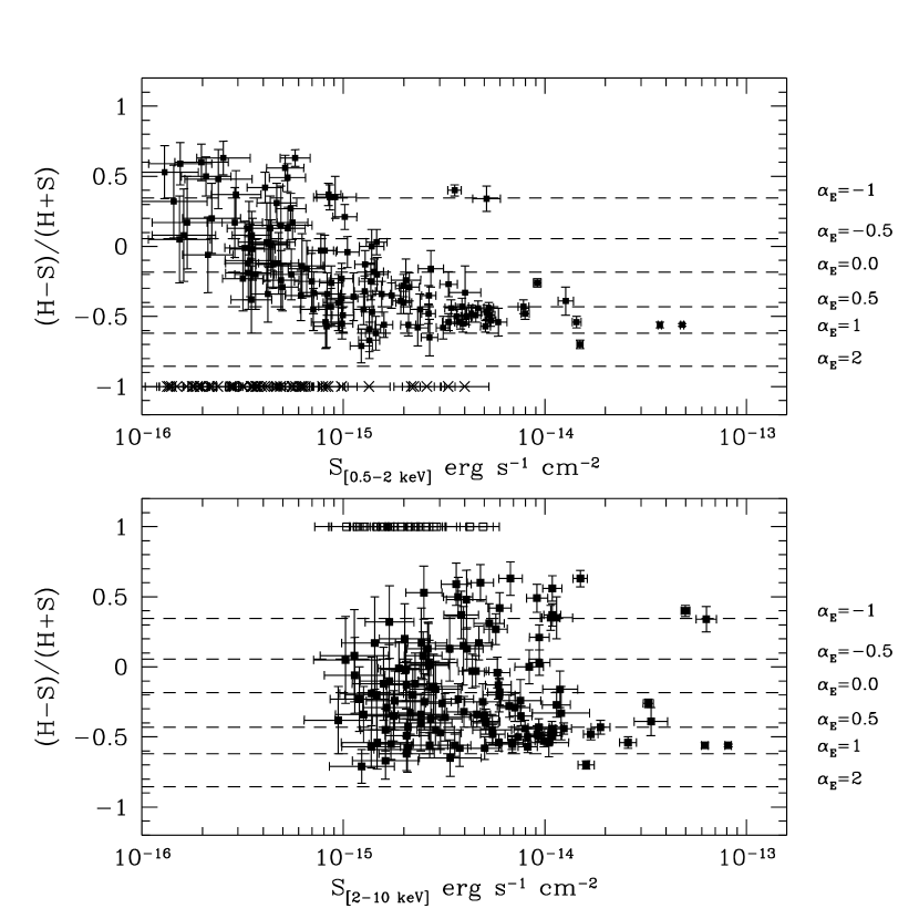
Figure 3: Hardness ratio for the sources detected in the soft and hard images as a function of the flux in the corresponding band. Sources detected only in the hard band are shown with open squares at HR$=1$, and the sources detected only in the soft band are shown with crosses at HR$=-1$. Dashed lines are power–law models with different energy index ($\alpha_{E}\equiv\Gamma-1$) computed assuming the Galactic value $N_{H}=8\times 10^{19}$ cm^-2 and convoluted with a mean ACIS–I response matrix at the aimpoint. Note that the number of hard sources increases at lower fluxes in both cases.

A more detailed view of the spectral properties as a function of the fluxes comes from the hardness ratio $HR=(H-S)/(H+S)$ where $H$ and $S$ are the net count rates in the hard (2–7 keV) and the soft band (0.5–2 keV), respectively. The distributions of the hardness ratios as a function of the soft and hard flux are shown in Figure 3. In both bands, the number of hard sources increases at lower fluxes. This is particularly significant if we plot the hardness ratio as a function of the hard fluxes. The average $HR$ ranges from $HR\simeq-0.2$ for $S>5\times 10^{-15}$ erg s^-1 cm^-2, to $HR\simeq 0.1$ for $S<5\times 10^{-15}$ erg s^-1 cm^-2. Such hardness ratio corresponds to an energy spectral index $\alpha_{E}=0$ and $\alpha_{E}=-0.5$ respectively. Even if we have already resolved the majority of the 2–10 keV background, the remaining fraction is made by a population of sources with progressively harder spectra.

There are 22 sources ($\simeq 11$% of the total sample) which are observed only in the hard band plotted at $HR=1$, and 51 sources ($\simeq$ 26% of the total sample) which are observed only in the soft band plotted at $HR=-1$. Studies from ASCA suggest that each source with nuclear activity is emitting in both bands at some level: the soft emission is $\geq 1$% of the hard emission for the hardest sources (Della Ceca et al. 1999a).

In the framework of the unification model for the AGNs, we expect to detect most of these sources in the soft and hard band if we push the detection limit down to low fluxes. We study the stacked spectra of the only–soft and the only–hard subsamples, to determine the flux level at which the single sources can be detected in the hard and soft bands respectively. For the sources detected only in the soft, the stacked spectrum has an hardness ratio of $HR\geq-0.67\pm 0.05$ and is well fitted by a power law with $\Gamma=2.2\pm 0.2$ for a $\chi_{\nu}^{2}\simeq 1.2$. This is consistent with the typical spectrum of unabsorbed TypeI AGN, similar to the sources found at very high fluxes by ASCA.

For the source detected only in the hard band, the hardness ratio of the cumulative spectrum is $HR\simeq 0.64\pm 0.09$. The fit with an unabsorbed power law gives $\Gamma=0.0\pm 0.2$, but with $\chi_{\nu}^{2}\simeq 2$. This indicates that a single power law is a bad fit and therefore intrinsic absorption is a necessary ingredient to describe the spectra of the faint, hardest sources. In fact, if we leave the local absorption free, we find $N_{H}=(2.5\pm 0.5)\times 10^{22}$ cm^-2, which is more than two orders of magnitude larger than the Galactic value, and a power law of $\Gamma=1.55\pm 0.3$ (errors correspond to the 90% confidence level). Such level of absorption correspond to $N_{H}>10^{23}$ cm^-2 for $z>1$. This results shows that the progessive hardening of the sources at faint fluxes is due to intrinsic absorption.

Moreover, the average hardness ratios derived for the two subsamples tell us that the average spectrum of the sources undetected in one of the two bands is similar to that of the other sources detected in both bands at low fluxes. In other words, we expect to detect most of them in a longer exposure. The average number of soft and hard counts for the sources detected in the hard or in the soft band only, is 3.8 and 4.1 respectively (corresponding to a count rate of $\simeq 1.3\times 10^{-5}$ cts/s).

The flux where the whole sample is detected in both the soft and the hard band will depend on the nature of the sources themselves. For example, the absorption detected in the only–hard subsample is already well in excess of $N_{H}=10^{22}$ cm^-2. If the intrinsic absorption is rapidly increasing with decreasing flux, as predicted by some AGN synthesis models (see Gilli, Salvati & Hasinger 2001), then the expected count rate of most of these hard sources can be much lower than the expected average $\simeq 1.3\times 10^{-5}$ cts/s and they could be undetectable in the soft band down to fluxes as low as $S\simeq 10^{-19}$ erg s^-1 cm^-2 (see discussion in §5).

In conclusion, at our present flux limits, we are still seeing significant differences in the soft and hard subsamples. These can result from an admixture of different classes of objects. This finding encourages us to push the flux detection threshold to the point where all the sources are detected in both bands. The value of such a flux can be much lower than expected depending on the intrinsic properties of the low–flux sources. This will be investigated with the total ($\sim$1Ms) exposure of the CDFS.

3.2 LogN–LogS and Total Flux from Discrete Sources

We now calculate the effective sky coverage at a given flux which is defined as the area on the sky where a source with a given net count rate can be detected with a $S/N>2.1$ in the extraction region defined in §2.1. The computation includes the effect of varying exposure, vignetting and point response function variation across the field. Such a procedure has been tested extensively with simulations performed with MARX v3.0, and it has been shown to be accurate to within a few percent (see panel d in Figure 1). The sky coverage is given in Figure 4. The step–like features are due to the large difference in the exposure across the field of view.

Using the sky–coverage we can compute the number counts in the soft and hard bands. In the soft band, shown in Figure 5, we find the Chandra results in excellent agreement with ROSAT in the region of overlap $S_{min}>10^{-15}$ erg s^-1 cm^-2. The Chandra data extend the results to $10^{-16}$ erg s^-1 cm^-2. A maximum likelihood fit to the soft sources gives

$$N(>S)=(400\pm 80)\Big{(}{{S}\over{2\times 10^{-15}}}\Big{)}^{-0.66\pm 0.06}\,\,\,\,\,\,{\rm cgs}$$ (1)

where the errors are at 1 sigma. The confidence levels at 1, 2 and 3 sigma for both slope and normalization are shown in the insert panel of Figure 5. The clear flattening with respect to the bright counts by ROSAT ($S>10^{-13}$ erg s^-1 cm^-2) shown in Paper I (also found by Mushotzky et al. 2000) is confirmed. The slope shows 2$\sigma$ evidence of further flattening with respect to the value found in Paper I. This difference may be partially due to the number of spurious sources and flickering pixels not removed in the previous data reduction, causing the soft number counts at the lowest fluxes to be overestimated by $\simeq 15$%. To check if the number counts are flattening in the investigated flux range, we perform a fit with a double power law for the differential number counts. The fit is done on 4 parameters: faint–end normalization and slope, bright–end slope and flux where the break occurs. We find that the differential counts are well fitted by a power law which is consistent with the euclidean slope at the bright end and with a slope $\alpha_{diff}\equiv\alpha+1=1.5\pm 0.1$ (1 sigma) at the faint end, with a break at $S=1.1\times 10^{-14}$ erg s^-1 cm^-2. Thus, below $S=10^{-15}$ erg s^-1 cm^-2, the slope of the cumulative number count is $\alpha\simeq 0.5$. Such a significant flattening will be further tested on the data from the 1Ms observation.

We compared our LogN–LogS with the predictions of the AGN population synthesis models described in Gilli, Salvati & Hasinger (2001). We consider their model B, where the number ratio R between absorbed and unabsorbed AGNs is assumed to increase with redshift from 4, the value measured in the local Universe, to 10 at $z\sim 1.3$, where R is unknown. This model was found to provide a better description of the X–ray constraints (ASCA and ROSAT number counts, luminosity function and redshift distribution by ROSAT, see Gilli, Salvati & Hasinger 2001) with respect to a standard model where R=4 at all redshifts. The value of R was independent of the luminosity and therefore a large population of obscured QSOs is included in the model. Such a model was originally calibrated to fit the background intensity measured by ASCA. In this paper, the parameters of the AGN X–ray luminosity functions assumed in the model B are recalibrated to fit the background intensity measured by HEAO–1. The predictions for the source counts (short dashed line in Figure 5) are in very good agreement with the Chandra LogN-LogS at all fluxes.

For the total contribution to the soft X–ray background, we refer to the 1–2 keV band, following Hasinger et al. (1993; 1998) and Mushotzky et al. (2000). In this energy band the comparison with the unresolved soft X–ray background is more straightforward than in the 0.5–2 keV band, since for energies $<1$ keV the Galactic contribution may be significant. The unresolved value in the 1–2 keV band measured by ROSAT is $4.4\times 10^{-12}$ erg s^-1 cm^-2, while the value found by ASCA is $3.7\times 10^{-12}$ erg s^-1 cm^-2 (see Hasinger et al. 1998 and references therein). We find a contribution of $\simeq 5.6\times 10^{-13}$ erg s^-1 cm^-2 deg^-2 for fluxes lower than $10^{-15}$ erg s^-1 cm^-2, corresponding to $\simeq 13-15$% of the unresolved flux. If this value is summed to the contribution at higher fluxes ($3.02\times 10^{-12}$ erg s^-1 cm^-2 deg^-2, see Hasinger et al. 1998), we end up with a total contribution of $\simeq 3.57\times 10^{-12}$ erg s^-1 cm^-2 deg^-2 for fluxes larger than $0.6\times 10^{-16}$ erg s^-1 cm^-2 (which is our flux limit in the 1–2 keV band), corresponding to 81% of the unresolved value as measured by ROSAT. If we assume the unresolved value measured by ASCA (which must be considered as a lower limit) the resolved contribution amounts to 96%.

We show the LogN–LogS distribution for sources in the hard band in Figure 6, down to a flux limit of $10^{-15}$ erg s^-1 cm^-2. The hard counts are normalized at the bright end with the ASCA data by Della Ceca et al. (1999b). A maximum likelihood fit to the hard sources data is:

$$N(>S)=(1150\pm 150)\Big{(}{{S}\over{2\times 10^{-15}}}\Big{)}^{-0.92\pm 0.12}\,\,\,\,\,\,{\rm cgs},$$ (2)

where the errors are at 1 sigma. We used a conversion factor for an average power law $\Gamma=1.4$. The confidence contours at 1, 2 and 3 sigma for the slope and the normalization are shown in the upper right corner of Figure 6. The hard number counts confirm the finding of Paper I (large filled dot) of a substantial flattening with respect to the slope at the bright end ($\alpha=1.67\pm 0.09$, Della Ceca et al. 1999b). We repeat the fit with a double power law in the differential counts, as in the case of the soft counts. For the hard counts too, we find evidence for further flattening: the differential counts are well fitted by a power law which is consistent with the euclidean slope at the bright end and with a slope $\alpha_{diff}=1.6\pm 0.2$ (1 sigma) at the faint end, with a break at $S=9\times 10^{-15}$ erg s^-1 cm^-2. To confirm such change in the slope below $S=10^{-14}$ erg s^-1 cm^-2 we need to extend the number counts to a lower flux limit.

The normalization computed at $2\times 10^{-15}$ erg s^-1 cm^-2 is consistent with the best fit in Paper I. Thus, we still find a difference larger than 3 sigma from the results of Mushotzky et al. (2000, large star). We stress that here we used an average spectral slope ($\Gamma=1.4$) flatter than in PaperI (where we used $\Gamma=1.7$). We chose the new value to be in agreement with the average spectral shape of our new combined sample. The short dashed line in Figure 6 is the same model as in Figure 5.

Despite the assumption of a flatter spectral slope, the difference in normalization with the hard number counts of Mushotzky et al. (2000) is still present. Our hard number counts are confirmed also by the results from the Lynx field, independently analysed by some of us, and from the XMM observation of the Lockman Hole (Hasinger et al. 2001a). The disagreement between us and Mushotzky et al. (2000) is statistically significant and acquires particular relevance since we are about to resolve completely the hard background. The causes of discrepancy may be due to calibration problems. A possible physical reason is cosmic variance. In this case the larger area of the CDFS should give a more accurate measure, if compared with the smaller area (1/4) covered by the pointing of Mushotzky et al. (2000).

The integrated contribution of all the sources within the flux range $10^{-13}$ erg s^-1 cm^-2 to $10^{-15}$ erg s^-1 cm^-2 in the 2–10 keV band is $(1.15\pm 0.15)\times 10^{-11}$ erg s^-1 cm^-2 deg^-2 for $\Gamma=1.4$. After including the bright end seen by ASCA for $S>10^{-13}$ erg s^-1 cm^-2 (Della Ceca et al. 1999b), the total resolved hard X–ray background amounts to $(1.46\pm 0.20)\times 10^{-11}$ erg s^-1 cm^-2 deg^-2. The inclusion of the ASCA data at bright fluxes minimizes the effect of cosmic variance. In Figure 7 we show the total contribution computed from the CDFS plus ASCA sample. The value at the limiting flux $S=10^{-15}$ erg s^-1 cm^-2 is still lower than the value of the total (unresolved) X–ray background $1.6\times 10^{-11}$ erg s^-1 cm^-2 deg^-2 from UHURU and HEAO-1 (Marshall et al. 1980). More recent values of the 2–10 keV integrated flux from the BeppoSAX and ASCA surveys (e.g., Vecchi et al. 1999; Ishisaki et al. 1999 and Gendreau et al. 1995) appear higher by 20-40%. These latest values are closer to the old Wisconsin measurements which were about 30% higher than the HEAO-1 value. The difference of 30% in flux has never been resolved up to the current day (McCammon & Sanders 1990).

Before concluding that a relevant fraction (10-40%)of the XRB has still to be resolved, we perform a detailed analysis of the hard sample, in order to understand if the resolved contribution may be underestimated due to a wrongly assumed spectral shape. To have a better understanding of how the spectrum of the X–ray background is built up at different fluxes, we divide the hard band sample into a bright subsample ($9\times 10^{-15}<S<10^{-13}$ erg s^-1 cm^-2), a faint subsample ($10^{-15}<S<9\times 10^{-15}$ erg s^-1 cm^-2) and a very faint subsample ($10^{-15}<S<4\times 10^{-15}$ erg s^-1 cm^-2) in terms of the hard fluxes. The sources were selected only in the area with 300ks of exposure, and the stacked spectra contain about 3300, 3700 and 1550 net counts respectively. We fitted the energy range from 1 keV to 10 keV with an absorbed power law and fixed the local absorption to the Galactic value $N_{H}=8\times 10^{19}$ cm^-2. The best–fit photon index is $\Gamma=1.55\pm 0.03$ for the bright sample, $\Gamma=1.26\pm 0.04$ for the faint sample, and $\Gamma=1.08\pm 0.07$ for the very faint sample (1 sigma errors). The trend, shown in Figure 8, is representative of the progressive hardening of the sources at lower fluxes. The line in Figure 8 is the prediction from the model used in Figures 5 and 6. Here we notice that at the very bright end our sample is dominated by few bright sources with a spectrum steeper than the rest of the sample, typical of the TypeI AGNs detected by ASCA at $S>10^{-13}$ erg s^-1 cm^-2 (which make about 30% of the hard background and have $\Gamma\simeq 1.8$). This may have biased the average spectral slope of our total sample towards slightly higher values. For example, the average spectral slope in the Lynx field, independently analyzed by some of us, in the same range of fluxes is $\Gamma=1.36\pm 0.02$ (1 sigma error) which is marginally flatter than $\Gamma=1.44\pm 0.03$ found in the CDFS.

We checked that using a varying $\Gamma$, as shown in Figure 8, does not alter the resulting logN–logS by more than a 5% increase in the normalization. The total contribution to the X-ray background changes even less, since the lower $\Gamma$ at low fluxes is compensated by the higher $\Gamma$ at high fluxes. We conclude that using an average $\Gamma=1.4$ to derive the hard fluxes from the net counts is justified. An interesting consequence of this analysis is that a fraction of at least $10$% of the unresolved hard XRB is still to be resolved at fluxes lower than $10^{-15}$ erg s^-1 cm^-2.

4 PROPERTIES OF SOURCES

The spectroscopic optical identification process of the X–ray sources described in this paper is still ongoing. Spectra have been taken with the FORS1 instrument on the VLT UT-1 in multislit mode. From about 130 spectra taken, we obtained a total of 99 redshifts, of which we regard 86 as secure.

The redshifts are distributed between $z=0.1$ and $z=3.7$ with 50 sources at $z\leq 1$ and 36 at $z>1$. In Figure 9 we plot the distribution as a function of redshift and hardness ratio. We notice a striking difference between the distribution of hard and soft sources. The large majority of the sources with $HR>0$ appear at $z\leq 1.6$, most of them at $z<1$. Moreover, most of the sources with $HR>0$ are identified as TypeII AGNs from the presence of narrow lines. TypeI AGNs instead, show an average $HR\simeq-0.5$ with a relatively narrow dispersion, and they are found in a broader range of redshift.

Only three sources have $HR\geq 0$ and $z>2$, including an obscured QSO at $z=3.7$ with $HR\simeq 0$. This source is marked with an asterisk in Figure 9 and is studied in detail in Norman et al. (2001). The average hardness ratio of all sources at $z>1.6$ is $HR\simeq-0.5$. This result, if confirmed by the complete analysis of the sample, would indicate that the hardest sources contributing to the 2–10 keV background are typically TypeII objects at $z\leq 1$, according to what has been found by Barger et al. (2001). Conversely, the most distant sources ($z>2$) have an average $HR\simeq-0.5$ and are prevalently TypeI objects. The dashed lines in Figure 9 show how the observed hardness ratio changes with redshift for a given intrinsic absorbing $N_{H}$ assuming a photon index $\Gamma=1.7$. We note that $HR$ is not a good tracer of intrinsic absorption especially at high $z$.

We can investigate in greater detail the nature of the hard sources. We selected a subsample of source with $HR>0$ (corresponding to an effective $\Gamma<0.5$ for a Galactic $N_{H}$). All the selected sources are included in the region with 300ks of exposure and have a hard flux lower than $2\times 10^{-14}$ erg s^-1 cm^-2. The sources selected in this way contribute about 20-30% of the total X–ray background. A fit with an absorbed power law gives $\Gamma=1.23\pm 0.13$ and $N_{H}=(1.3\pm 0.2)\times 10^{22}$ cm^-2 (1 sigma errors). Using an average redshift of $\langle z\rangle\sim 0.7$ as representative of the sources in the subsample, we find an average intrinsic absorption corresponding to $N_{H}\simeq(4\pm 0.4)\times 10^{22}$ cm^-2 with a similar $\Gamma$. This confirms the presence of strong intrinsic absorption for the hardest sources detected at low fluxes.

Luminosities are computed in the rest–frame soft band after assuming an average power law spectrum with $\Gamma=1.4$, in a critical universe with $H_{0}=50$ km/s/Mpc. The distribution of luminosities emitted in the soft band with redshift is shown in Figure 10. This plot shows that in 300ks we have achieved a greater sensitivity than all previous surveys. The upper solid line corresponds to a sensitivity limit in flux of $2\times 10^{-16}$ erg s^-1 cm^-2, that was the flux limit of the 120k exposure (see Paper I). Most of the sources with $HR>0$ appear to fall in the $L_{hard}=10^{42}-10^{44}$ erg s^-1 range and are identified with TypeII absorbed AGNs. Data obtained with the HST observations of a small fraction of our field (Schreier et al. 2001) will address in detail the morphological properties of the optical counterparts.

Softer sources with $HR<0$ appear to span the range from $10^{40}$ to $10^{45}$ erg s^-1. At luminosities larger than $10^{42}$ erg s^-1 these sources are mostly identified with TypeI AGN. At the low luminosity end, several sources are detected only in the soft band ($HR=-1$). Most of these objects are identified with galaxies at redshift less than $0.6$ with soft luminosities restricted to a range between $L_{x}=10^{40}$ and $L_{x}=10^{42}$ erg s^-1. This population of relatively nearby galaxies with soft X–ray spectra has been found also by Hornschemeier et al. (2001) in the Chandra Deep Field North.

In the plot $S$ versus $R$, where S is the X–ray flux in the soft band (see Figure 7 of Paper I) this subsample appears to populate the low $S/R$ region at fluxes $S<10^{-15}$ erg s^-1 cm^-2. We can use a criterium defined in the $S$–$R$ plane to isolate this soft, low luminosity population of sources. If we define a subsample requiring $S/S_{opt}<0.1$, $S_{tot}<3\times 10^{-15}$ erg s^-1 cm^-2, and $HR<-0.5$, we find 18 sources. Among these 18 sources, 10 have redshift, with an average value $\langle z\rangle=0.25$. The very high redshift sources with $HR=-1$ (see Figure 9) have $S/S_{opt}\simeq 1$ and are therefore excluded from this subsample. By visual inspection from the images in the $R$ and $B$ bands, at least 10 of these 18 sources appear clearly to be galaxies. If we fit their stacked spectrum with a power law, we find consistency with Galactic absorption, and a spectral slope $\Gamma=2.0\pm 0.2$ (90 % c.l.). If we repeat the fit with a thermal spectrum, we find a temperature of $3.5\pm 1.5$ keV, which is too high to be produced by hot gas in the potential wells of galaxies. Such an apparent temperature may be due to the contribution of low luminosity nuclear activity or a population of X–ray binaries. Both fits have a $\chi_{\nu}^{2}\simeq 1$. A better definition of the subsample will be available when the spectroscopic optical identification is completed.

5 CONCLUSIONS

We detected X–ray sources down to a flux limit of $10^{-16}$ erg s^-1 cm^-2 in the 0.5–2 keV soft band and $10^{-15}$ erg s^-1 cm^-2 in the 2–10 keV hard band, improving the sensitivity by a factor of 2 with respect to Paper I. The LogN–LogS relationship of the hard sample confirmed the previous findings obtained from the 120 ksec exposure (Paper I). The average slope turns out to be $\alpha=0.92\pm 0.12$, which is flatter with respect to the quasi–euclidean slope found by ASCA at the bright end ($S>10^{-13}$ erg s^-1 cm^-2). However, adopting a fit with double power law in the whole flux range, we find indication for flattening down to $\alpha=0.6\pm 0.2$ below $S\simeq 10^{-14}$ erg s^-1 cm^-2.

After the inclusion of the ASCA sources at the bright end, the total contribution to the resolved hard X–ray background down to our flux limit of $10^{-15}$ erg s^-1 cm^-2 now amounts to $(1.45\pm 0.15)\times 10^{-11}$ erg cm^-2 s^-1 deg^-2. This result is robust to variations of the average spectral slope in the hard sample, which can be as low as $\Gamma=1.1$ for the faintest sources. The value for the unresolved X–ray background ranges from $1.6$ to $2.4\times 10^{-11}$ erg s^-1 cm^-2, so a fraction between 60% and 90% of the hard XRB has now been resolved.

We confirm our previous finding on the average spectrum of the sources of the total sample, which can be well approximated with a power law with index $\Gamma=1.4$. We also find a progressive hardening of the sources at lower fluxes, both for the soft and the hard samples. In particular, we divided the hard sample into three subsamples: bright ($9\times 10^{-15}<S<10^{-13}$ erg s^-1 cm^-2), faint ($10^{-15}<S<9\times 10^{-15}$ erg s^-1 cm^-2) and very faint ($10^{-15}<S<4\times 10^{-15}$ erg s^-1 cm^-2). The average power law is $\Gamma=1.55\pm 0.03$ for the bright subsample, $\Gamma=1.26\pm 0.04$ for the faint subsample, $\Gamma=1.08\pm 0.07$ for the very faint subsample. The progressive hardening at faint fluxes is probably due to a stronger intrinsic absorption.

In the soft band the counts show a slope of $\alpha=0.66\pm 0.06$ (1 sigma error), clearly flatter than the slope at the bright end measured by ROSAT. A double power law fit indicates a progressive flattening at the faint end, with a best fit with $\alpha=0.5\pm 0.1$ for fluxes below $10^{-15}$ erg s^-1 cm^-2. The soft X–ray background in the energy range 1–2 keV is now resolved at the level of 81–96 % depending on the assumed value for the unresolved soft XRB.

The soft and the hard LogN–logS must ultimately approach each other. In fact, in the unified AGN explanation of the XRB we should, with increasing sensitivity, see the same objects in both bands. However, if the remaining hard population is constituted by sources that are even more strongly absorbed, there will be a significant fraction of hard sources still undetected in the soft band also at $S\simeq 10^{-17}$ erg s^-1 cm^-2. Following the model B in Gilli, Salvati & Hasinger (2001), we found that the soft and hard LogN–LogS predict the same source density at $S\sim 10^{-19}-10^{-20}$ erg s^-1 cm^-2.

We have also used measured redshifts for 86 sources. The spectra will be presented in the catalog paper of the 1Ms exposure (Giacconi et al, in preparation). We find that the hard sources with $HR>0$ are typically found at $z<1$, with intrinsic luminosities between $10^{42}$ and $10^{44}$ erg s^-1 in the soft band. Between the objects producing the 2–10 keV X–ray background, the ones with $HR>0$ (producing between 20–30% of the total XRB) appear relatively nearby (redshifts $z<1$) and are most easily identified with Seyfert II galaxies (see also Barger et al. 2001). We note that a bias could be present against obscured AGNs, since our spectroscopically identified sample is not complete and obscured AGNs are expected to have on average fainter magnitudes than the unobscured ones. One of the important results of Chandra is the detection of obscured QSOs. A first clear example of hard (i.e. likely obscured) X–ray sources at high redshift with X–ray luminosities above $3\times 10^{44}$ erg s^-1 have been already found (see Figure 9). This source is extensively described in Norman et al. (2001). When the optical identification program will be completed, it will be possible to test whether the population of aborbed AGN is as large as assumed in the AGN synthesis models of the XRB (Madau, Ghisellini & Fabian 1993; Comastri et al. 1995; Gilli et al. 2001, Comastri et al. 2001).

The observation at $S<10^{-15}$ erg s^-1 cm^-2 of very soft ($HR<-0.5$) objects with $L_{X}$ between $10^{40}$ and $10^{42}$ erg s^-1 up to $z\simeq 0.3$ opens up a new window to the study of the evolution of galaxies at moderate $z$. A large number of galaxies could increase the number counts at low fluxes without contributing significantly to the XRB.

Figure 1: Analysis of one of the simulations performed with MARX for the 300ks exposure. We show the measured counts vs input counts for each source (panel a); the difference between the input source positions and the measured positions (panel b); the relative errors on the detected counts as a function of the S/N ratio (panel c); the output vs the input number counts (panel d). This analysis refers to the soft band.

Figure 2: Stacked spectrum of the total sample of sources in the CDFS, fitted in the energy band $1-8$ keV with an absorbed power law with column density fixed to the Galactic value $N_{H}=8\times 10^{19}$ cm^-2. The best fit slope is $\Gamma=1.44\pm 0.03$ (errors at 90% c.l.) for a $\chi_{\nu}^{2}=1.16$, in agreement with the average slope of the unresolved hard X–ray background. The solid line is the best–fit model, while the lower panel shows the standard deviations in each energy bin.

Figure 4: Sky coverage of the 300ks exposure of the Chandra Deep Field South for the soft (dashed line) and the hard (solid line) band, as a function of the soft and hard fluxes respectively. Note that the hard energy flux is computed in the 2–10 keV band, while the sky coverage refers to the 2-7 keV image. The step–like features are due to the different roll angles in the 4 observations that produce corners with different exposure times.

Figure 5: The LogN–LogS in the soft band from the Chandra Deep Field South for an average spectral slope $\Gamma=1.4$ (filled squares). Dashed lines are the counts from ROSAT observation of the Lockman Hole (Hasinger et al. 1998), and the dotted contour is the extrapolation from the fluctuation analysis in ROSAT data (Hasinger et al. 1993). The upper and lower solid lines indicate uncertainties due to the sum of the Poisson noise (1 sigma) including the uncertainty in the conversion factor (see text). The short dashed line is from model B in Gilli, Salvati & Hasinger (2001), rescaled to fit the total background measured by HEAO–1 (see text). The insert shows the maximum likelihood fit to the parameters in the LogN–LogS fit $N(>S)=K_{15}(S/{2\times 10^{-15}})^{-\alpha}$. The contours correspond to $1\sigma$, $2\sigma$ and $3\sigma$. The star is the fit from Mushotzky et al. (2000) at $S=2\times 10^{-15}$ erg s^-1 cm^-2; the error bar is their quoted 68 % confidence level. The large dot is the result from the 120k exposure (for $\Gamma=1.4$).

Figure 6: The LogN–LogS in the hard band from the Chandra Deep Field South for an average spectral slope $\Gamma=1.4$, symbols as in Figure 5. The open circle at high fluxes is from ASCA and Beppo SAX (Giommi, Perri & Fiore 2000, Ueda et al. 1999) and the continuous line is the fit to the counts from ASCA in the range $10^{-12}-10^{-13}$ erg cm^-2 s^-1 (Della Ceca et al. 1999b). The upper and lower solid lines indicate uncertainties due to the sum of the Poisson noise (1 $\sigma$) including the uncertainty in the conversion factor (see text). The insert shows the maximum likelihood fit to the parameters in the LogN–LogS fit $N(>S)=K_{15}(S/{2\times 10^{-15}})^{-\alpha}$. The thick contours correspond to $1\sigma$, $2\sigma$ and $3\sigma$. The star is the fit from Mushotzky et al. (2000) at $S=2\times 10^{-15}$ erg s^-1 cm^-2; the error bar is their quoted 68 % confidence level. The large dot is the result from the 120k exposure (for $\Gamma=1.4$). The dashed line is the same model of Figure 5.

Figure 7: The contribution to the hard X–ray flux density as a function of the flux of the resolved sources. The total resolved contribution is computed from the CDFS sample plus the bright sample from ASCA at fluxes larger than $\simeq 10^{-13}$ erg s^-1 cm^-2 (Della Ceca et al. 1999b). The upper dashed lines refer to previous measures of the hard X–ray background; from bottom to top: Marshall et al. (1980, HEAO-1), Ueda et al. (1999, ASCA1), Ishisaki (1999, ASCA2), Vecchi et al. (1999, BeppoSAX).

Figure 8: The average power law index of the stacked spectra of the bright, faint and very faint subsamples of the sources detected in the hard band, as defined in the text. Errors on $\Gamma$ refer to the 90% confidence level. The local absorption has been fixed to the Galactic value $N_{H}=8\times 10^{19}$ cm^-2. The line is derived from the same model of Figure 5 and 6.

Figure 9: Hardness ratio as a function of redshift for the 86 sources with optical spectra in our sample. TypeI AGNs are marked with large open circles; TypeII with open squares; galaxies with triangles. Objects with uncertain type identification are marked with small circles. The dashed lines show how the hardness ratio change with $z$ for a given intrinsic absorbing column assuming a photon index $\Gamma=1.7$. The horizontal solid line is the average hardness ratio of the total XRB ($\Gamma=1.4$). The source marked with a star is the absorbed QSO discussed in Norman et al. (2001).

Figure 10: $L_{X}$ in the soft band (rest frame) versus redshift for the Chandra sources. Symbols as in Figure 9. The two solid lines correspond to a flux limit of $2\times 10^{-16}$ erg cm^-2 s^-1 (upper line, the flux limit of the previous 120 ks exposure) and to $2\times 10^{-17}$ erg cm^-2 s^-1 (lower line), assuming a spectral slope $\Gamma=1.4$. A critical universe with $H_{0}=50$ km/s/Mpc has been assumed.

References

- (1) Appenzeller I., et al. 1998, ESO Messenger, 1, 94
- (2) Arnouts, S., et al. 2001, A&A submitted, astro-ph/0103071
- (3) Baade, D., et al. 1999, ESO Messenger, 15, 95
- (4) Barger, A. J.; Cowie, L. L.; Mushotzky, R. F.; Richards, E. A. 2001, AJ, 121, 662
- (5) Bertin, E., Arnouts, S. 1996, A&A Supplement, 117, 393
- (6) Brandt, W.N., et al. 2001, astro-ph/0102411
- (7) Comastri, A., Setti, G., Zamorani, G., & Hasinger, G. 1995 A& A, 296, 1
- (8) Comastri, A., Fiore, F., Vignali, C., Matt, G., Perola, G.C. & La Franca, F. 2001, MNRAS submitted, astro-ph/0105525
- (9) Della Ceca, R., Castelli, G., Braito, V., Cagnoni, I. & Maccacaro, T. 1999a, ApJ, 524, 674
- (10) Della Ceca, R., Braito, V., Cagnoni, I. & Maccacaro, T. 1999b, astro-ph/0007430
- (11) Freeman, P.E., Kashyap, V., Rosner, R., & Lamb, D.Q. 2001, ApJ submitted
- (12) Gendreau, K.C., et al. 1995 Publ. Astron. Soc. Jpn. 47, L5-L9
- (13) Giacconi, R., Rosati, P., Tozzi, P., et al. 2001, ApJ in press (Paper I)
- (14) Gilli, R., Salvati, M., & Hasinger, G. 2001, A&A, 366, 407
- (15) Giommi, P., Perri, M., & Fiore, F. 2000, A&A, 362, 799
- (16) Hasinger, G., Burg, R., Giacconi, R., Hartner, G., Schmidt, J., Truemper, J., & Zamorani, G. 1993, A&A 275, 1
- (17) Hasinger, G., Burg, R., Giacconi, R., Schmidt, J., Truemper, J., & Zamorani, G. 1998, A&A 329, 482
- (18) Hasinger, G., et al. 2001a, A&A 365, L45
- (19) Hasinger, G., et al. 2001b, in preparation
- (20) Hornschemeier, A.E., et al. 2000, ApJ, 541, 49
- (21) Hornschemeier, A.E., et al. 2001, astro-ph/0101494
- (22) Ishisaki, Y., Makishima, K., Takahashi, T., Ueda, Y., Ogasaka, Y., & Inoue, H. 1999, ApJ submitted
- (23) Madau, P., Ghisellini G., & Fabian, A. C. 1993, ApJ, 410, L7
- (24) Marshall, F. et al. 1980, ApJ, 235, 4
- (25) McCammon, D., & Sanders W.T. 1990, ARA&A 28, 657
- (26) Mushotzky, R.F., Cowie, L.L., Barger, A.J., & Arnaud, K.A. 2000, Nature, 404, 459
- (27) Norman, C., et al. 2001, ApJ submitted, astro-ph/0103198
- (28) Rosati, P., Della Ceca, R., Burg, R., Norman, C., Giacconi, R. 1995, ApJL, 445, 11
- (29) Rosati, P., et al. 2001, in preparation
- (30) Schreier, E., et al. 2001, ApJ in press, astro-ph/0105271
- (31) Ueda, Y., et al. 1999, ApJ, 518, 656
- (32) Vandame, B., et al. 2001, A&A submitted, astro-ph/0102300
- (33) Vecchi, A., Molendi, S., Guainazzi, M., Fiore, F., & Parmar, A.N. 1999, A&A, 349, 73
- (34) Wise, M. W., Davis, J. E. , Huenemoerder, D. P. , Houck, J. C. and Dewey, D. 2000, MARX technical manual, http://space.mit.edu/ASC/MARX/manual/manual.html