Mapping of the SZ effect in the cluster Cl 0016+16 with the Ryle Telescope

Abstract

We have mapped the high-redshift (z = 0.546) cluster Cl 0016+16 with the Ryle Telescope at 15 GHz. The Sunyaev–Zel’dovich decrement is clearly detected, and resolved. We combine our data with an X-ray image from Rosat, and a gas temperature from Asca to estimate the Hubble Constant $H_{0}=69^{+21}_{-16}~{}\rm km\ s^{-1}\ Mpc^{-1}$ for an $\Omega_{M}=1.0$ cosmology or $H_{0}=84^{+25}_{-19}~{}\rm km\ s^{-1}\ Mpc^{-1}$ for $\Omega_{M}=0.3$ and $\Omega_{\Lambda}=0.7$.

1 Introduction

The cluster Cl 0016+16 lies at a redshift of 0.546 [Dressler & Gunn 1992], and in X-rays is one of the most luminous clusters known [Henry et al. 1992]. Despite its high redshift it has a predominance of red galaxies (i.e. it defies the Butcher–Oemler effect [Butcher & Oemler 1984]). There is also evidence that it is undergoing a merger; the galaxy distribution is distinctly bimodal, and a map of the total mass derived from weak lensing of background galaxies [Smail et al. 1995] shows several peaks, although the X-ray emission appears somewhat smoother [Birkinshaw & Hughes 1994].

Cl 0016+16 was also one of the first clusters in which the Sunyaev–Zel’dovich (SZ, Sunyaev & Zel’dovich [Sunyaev & Zel’dovich 1972]) effect was detected [Birkinshaw et al. 1984]. It has been subsequently mapped with the OVRO/BIMA array at 28–30 GHz [Carlstrom et al. 1996] and detected at 2.1 mm and 1.2 mm with the Diabolo experiment at the IRAM-30 m telescope [Desert et al. 1998]. Here we present Ryle Telescope (RT) observations of the SZ effect in Cl 0016+16 and provide an image of its two-dimensional structure. We then combine this data with the Rosat PSPC image and Asca temperature data to calculate the Hubble constant.

2 SZ Observations with the Ryle Telescope

The RT is an east–west aperture synthesis telescope specifically designed to map low-surface-brightness structures in the microwave background [Jones 1991]. Five of its eight antennas are used in close-packed configurations to provide the high temperature sensitivity needed to map the SZ effect. The system temperature at 15 GHz is 60 K, giving a flux sensitivity in 12 h of 200 $\mu{\rm Jy\;beam^{-1}}$. The RT correlator provides 35 spectral channels of approximately 10 MHz bandwidth each (7 synthesised channels in each of 5 IF sub-bands).

We have made many detections of the SZ effect with the RT [Jones et al. 1993, Grainge et al. 1993, Jones 1995, Saunders 1995]; we will first describe in some detail the general observing procedure, and then discuss the Cl 0016+16 observations.

2.1 General observing procedure

Clusters are observed in runs of 12 hours with the telescope in one of the compact configurations shown in table 1. In the case of fields of declination less than $48^{\circ}$ with the RT in configuration Ca or Cb, the observation is curtailed when none of the baselines of the compact array remain unshadowed. Due to the east-west nature of the RT, this results in a gap along the v-axis in the aperture plane coverage. To fill this region we also observe in either Cc array (for $24^{\circ}<\rm{dec}<48^{\circ}$) or Cd array (for $16^{\circ}<\rm{dec}<24^{\circ}$). The pointing centre chosen for each observation is the position of the peak of the X-ray emission from the cluster. For each observation, a bright ($>0.2$ Jy) nearby point source is chosen as a phase calibrator and is observed for either five or ten 32-second samples (depending on its brightness), for every 30 samples on-source. A primary calibrator, either 3C48 or 3C286, is observed either before or after a run.

2.2 Editing the data

The Postmortem package  [Titterington 1991] is used for editing and calibrating of RT data. The performance of the RF system is monitored by the use of a modulated noise source at each feed-horn. Corrections to the data and their weights are applied to take account of variations in system noise, mainly a result of weather conditions. Exceptionally bad data are discarded, along with that during winds in excess of 20 knots (marginal pointing) and during slewing and settling while changing pointing centres, and for any baseline actually, or close to being, shadowed.

2.3 Primary calibration

The absolute flux scale of the RT is fixed on 3C48 and 3C286. Flux densities of 1.70 and 3.50 Jy (Stoke’s $I-Q$) are assumed for these respectively [Baars et al. 1977]. We calculate a set of complex gains to apply to every sub-band and channel of each antenna from the primary calibrator observations. A least-squares algorithm is used to derive the gains for each antenna from the data for each baseline. This means that data from many baselines are used to calibrate each antenna, and increases the signal-to-noise of the calibration. The amplitude scale is observed not to drift significantly over the timescale of individual observations, and so is calibrated with a single correction for each observation. This primary calibration is then applied to the data from the main observation. Monitoring by the VLA has detected low level variability in both of these sources on long time-scales [VLA calibration manual 1996], and we apply a separate correction for these changes.

2.4 Phase calibration

Antenna-based phase corrections are calculated for each of the 5- or 10-sample secondary calibrator observations, and interpolated to correct the source phases. This removes phase drifts due to the atmosphere and local oscillator distribution, which can be up to $360^{\circ}$ during a 12-hour run for the longer baselines of the compact array. Since phase differences between channels in the same sub-band are relatively constant, and are calibrated out using the flux calibrator observations, we merge the visibilities of the 7 channels for each sub-band and smooth over all 5 or 10 samples within the particular calibrator pointing in order to increase the signal-to-noise ratio of the calibration. We do not merge the secondary calibrator visibilities over the sub-bands since we have found that during a 12-hour run the different sub-bands can drift by up to  $5^{\circ}$. Closure phase errors are calculated when the antenna solutions are found, and are almost always consistent with the thermal noise. The data are flagged where this is not the case. In order to check the secondary calibration the visibilities are smoothed, their mean amplitudes and phases are examined and the data for one representative channel are plotted out. We pick out and flag anomalous mean amplitudes, phases and their rms, and look for amplitude or phase jumps caused by interference or possible hardware faults.

2.5 Smoothing, weighting and interference clips

The data are smoothed to an integration time appropriate to the resolution of the array: 320 s for the most compact arrays Ca, Cb and Cc, and 96 s for array Cd. These smoothing periods were chosen to ensure that $R_{a}$, the fractional decrease in the peak response to a point source is close to unity. $R_{a}$ is given by (see e.g. Thompson [Thompson et al. 1986])

$$R_{a}\approx 1-{1\over 3}\left({{0.833\omega_{e}\tau_{a}r}\over{\theta_{b}}}\right)^{2},$$ (1)

where $\omega_{e}$ is the rotation rate of the Earth, $\tau_{a}$ is the averaging time, $\theta_{b}$ is the FWHM of the synthesised beam, and $r$ is the distance of the point source from the observation centre. For the smoothing periods used, a point source 6 arcminutes from the pointing centre (the position of the first null of the RT primary beam response) will have $R_{a}\geq 0.99$ on the longest baseline available in the respective configurations. Any low-level interference is removed by a simple clip at 0.25 Jy before smoothing, and at 0.079 Jy after smoothing over 10 samples, or at 0.144 Jy after smoothing over 3 samples. This corresponds to approximately 3 standard deviations. The visibilities are weighted by their inverse variances, calculated from the product of the system temperatures of the two antennas and are then written out in fits format to be transferred to Aips. As a final check of our calibration procedure, each day’s data are mapped individually using the entire uv-range and natural weighting, in order to give maximum signal to noise. We examine these maps for artifacts due to poor calibration and interference which have not been removed.

2.6 Data analysis

Before a map of the SZ effect can be made, the effects of discrete sources on the data have to be removed. The clusters we have studied have been pre-selected to be radio-quiet, but may contain several radio sources with flux densities of up to a few mJy. Rather than attempt to identify and determine the fluxes of these sources in the map plane through Cleaning the long baseline data as has been our practice previously [Grainge et al. 1993, Jones et al. 1993], we now fit directly to the visibilities in the aperture plane using the program Fluxfitter. This procedure is explained in greater depth in Grainger et al. [Grainger et al. 2001]. We subtract the sources from the original uv-data using point-source models, implemented by the Aips task Uvsub. The procedure that we adopt for removing sources which are not point sources on our longest baselines, but are not extended on the scale of the SZ decrement, is detailed in Grainge et al [Grainge et al. 1996]. If we find a bright source which is extended on the scale of the SZ effect, we cannot be confident of subtracting the source accurately and observations of the field have to be abandoned.

The SZ decrement is typically several arc-minutes in extent and so is resolved out by the long-baseline antenna pairs, and to a good approximation is only detected by the short baselines. We therefore either map only the short baseline source-subtracted data (typically 0–1 k$\lambda$), or apply a uv-taper to look for an SZ decrement close to the X-ray cluster centre. The quality of the resulting image is determined by both the structure of the SZ decrement and the aperture-plane coverage of the observation. For high-declination objects, e.g. Abell 2218 [Jones 1995] or Abell 773 [Grainge et al. 1993], the aperture-plane coverage is basically a circular ring at the radius of the shortest baseline, with very little SZ signal at the second-shortest baseline. An image made from this will show the position of the centre of the decrement and reveal any significant departures from circular symmetry, but does not strongly constrain the shape of the SZ profile. Additional information, such as X-ray imaging and assumptions about the physics of the gas, must be used to fully model the gas structure. In a low-declination object such as Cl 0016+16 however, the projection of the baselines results in a much better-filled aperture plane. Using two different array configurations optimised for the north–south and east–west parts of the aperture plane results in an image in which significant structure can be seen. Since the SZ signals generally have only moderate signal-to-noise ($\sim 5\sigma$), Cleaning to remove the point-spread-function has to be performed with great care. With the poor aperture-plane coverage used for the mapping, the inner part of the synthesised beam is poorly represented by the Gaussian restoring beam, with the result that the map’s noise level will be artificially reduced, and that significant artifacts can occur. The best results are obtained by using a Clean -box around the decrement, followed by a Clean over the entire field, but never cleaning deeper than about $2\sigma$.

Cleaned maps of the SZ effect are useful for showing whether we have detected any resolved structure in the decrement, and for overlaying on X-ray or optical images to check for positional coincidence. However, it is necessary to do all analysis for calculation of $H_{0}$ in the aperture plane [Grainge et al. 2001], since the noises are independent between visibilities, as opposed to the map plane in which the pixel noises are strongly correlated.

3 RT Observations of Cl 0016+16

Two array configurations were used: the most compact array, Cb, which provides short baselines at hour angles around zero, but in which the antennas shadow each other at extreme hour angles, and a more extended array, Cd, to provide unshadowed north–south baselines. Figure 1 shows the aperture-plane coverage. The asymmetry is due to the $\sim 3^{\circ}$ offset of the baselines from east–west. The cluster was observed for the total of 46 days in the most compact array, and 32 days in the more extended array, between 1993 July 20 and 1995 January 10 with simultaneous observations of 0007+171 as a phase calibrator. The pointing centre was $\rm 00^{h}15^{m}58^{s}.5+16^{\circ}09^{\prime}42^{\prime\prime}$ (B1950.0), which was also the phase centre. Previous long integrations with the RT have shown that it does not suffer from systematic offsets at the phase centre.

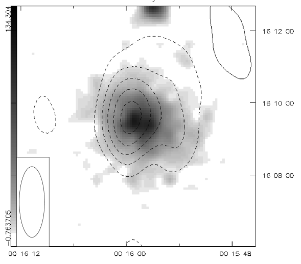
Figure 2: High resolution RT map of the SZ effect in Cl 0016+16 (contours) superposed onto the Rosat PSPC image. The contours are -250, -200, -150, -100, -50 and 50 $\mu$Jy. The restoring beam is $143\times 51^{\prime\prime}$ at an angle of $4.3^{\circ}$. The rms pixel noise on the map is $40~{}\mu$Jy. The entire source-subtracted data set has been used to produce this map, with a Gaussian taper with $1/e$ points at 2 k$\lambda$.

A map of the long-baseline data detected the presence of two sources in the field. Both of these correspond with sources in the survey of Moffet & Birkinshaw[Moffet & Birkinshaw 1989] (hereafter MB). The only other source within $6^{\prime}$ (the RT primary beam) of our pointing centre that was detected by MB is source MB14, the extended cluster halo emission. This will be discussed further in section 4.3. Fluxfitter was run over the two array configurations separately (because of the possibility of source variability as discussed in Grainge et al. [Grainge et al. 1996]), and the results are shown in table 2. Once these sources had been subtracted we mapped and Cleaned the entire data set at two different resolutions (Figures 2 and 3). These maps show clear detections of the SZ decrement and the high–resolution image has a resolved east–west extension. The position of the peak and the extent of the SZ decrement agree well with the X-ray emission.

4 Determining The Hubble Constant

The method we use to measure $H_{0}$ from RT cluster data has been described in detail by Grainge et al [Grainge et al. 2001]. As in that paper we make our models assuming an Einstein-de Sitter cosmology, and then calculate corrections for other cosmologies. Here we give details relevant to Cl 0016+16.

4.1 X-ray image

We use the public Rosat PSPC image of Cl 0016+16 (PI Hughes), with live time of 43157 s, to fit for the shape of the gas density distribution in the cluster and to determine a value of $n_{0}^{2}/H_{0}$. We use the 0.5–2 keV band to minimise the effect of galactic emission and absorption; for the later we assume a column density of $5.6\times 10^{20}\rm\,cm^{-2}$. We fit to a two-dimensional $\beta$-model using Poisson statistics as the number of counts per pixel is typically small, and excluding regions containing X-ray point sources. We estimate the mean background level in a $15^{\prime\prime}$ pixel to be $4.04\times 10^{-5}$ counts $\rm s^{-1}$. We find best-fit parameters of $\beta=0.714$, core radii of $40.8^{\prime\prime}$ and $32.9^{\prime\prime}$ at a position angle of $53^{\circ}$ and a central electron density of $n_{0}=1.373\times 10^{4}\,h^{1/2}\rm~{}m^{-3}$, where $H_{0}=100h\,\rm km^{-1}Mpc^{-1}$, assuming that the line-of-sight depth through the cluster is the geometric mean of the two elliptical axes in the plane of the sky and an X-ray emission constant of $3.80\pm 0.27\times 10^{-69}$ $\rm counts~{}s^{-1}$ from 1 m³ of gas of electron density 1 m^-3 at a luminosity distance of 1 Mpc. These are in good agreement with the two-dimensional models of Hughes & Birkinshaw [Hughes & Birkinshaw 1998], who use a very similar fitting method, and also with those of Neumann & Böhringer [Neumann & Böhringer 1997], who fit with a $\chi^{2}$ statistic after a Gaussian smoothing.

Figure 4 shows the Rosat PSPC image, our X-ray model, and the residuals from our fit. The reduced value of $\chi^{2}$ for this fit is 0.945. However, since the data are Poisson distributed with a relatively low mean for many pixels, approximating the distribution to be Gaussian is a poor assumption and therefore $\chi^{2}$ is not the correct statistic to use. We attempt to evaluate the goodness of fit by using the mean of the log likelihoods of each pixel, given the model, over the image. From our model we calculate 100 realisations of the image using the Poisson distribution with the appropriate mean at each pixel, and find the distribution of $L$ to be ${L}=-2.339\pm 0.034$. The corresponding value for the Rosat image is ${L}=-2.32$. We therefore conclude that the fit is a good one.

4.2 X-ray temperature

We adopt the X-ray temperature calculated by Hughes & Birkenshaw [Hughes & Birkinshaw 1998] of $7.55^{+0.72}_{-0.58}$ keV. We assume the cluster to be isothermal at this temperature. The effect of this probably inaccurate assumption on our estimate of $H_{0}$ is discussed in Maggi et al. [Maggi et al. 2001].

4.3 Cluster halo emission

Giovannini & Feretti [Giovannini & Feretti 2000] have mapped the cluster halo source MB14 with the VLA in B, C and D array at L-band (1.4 GHz). These measurements give access to short enough baselines to ensure that the full flux density has been found and has not been resolved out. They find that the total integrated flux from this extended source is 5.5 mJy. Assuming that the halo has a similar spectrum to that found in A665 [Jones and Saunders1996] we estimate that the halo’s flux density will have fallen to 55 $\mu$Jy by 15 GHz. We model the halo emission as a Gaussian with FWHM $2^{\prime}$ in order to estimate the extent to which we will resolve out the extended emission. We find that only $51\pm 9\%$ of the total zero-spacing flux is detected by the RT shortest baseline of $870~{}\lambda$.

The effect that halo emission will have on our calculation of $H_{0}$ is to reduce the flux density of the detected SZ effect, which will lead to an overestimate of $H_{0}$ by $(S_{halo}/S_{SZ})^{2}~{}\%$. Estimating that the SZ decrement detected by the RT has been reduced by $30\pm 30~{}\mu$Jy we apply a correction of $-7\pm 7\%$ to our value of $H_{0}$.

4.4 $\bf H_{0}$ from Cl 0016+16

Combining our X-ray model and SZ data in the aperture plane we find a maximum likelihood fit of $H_{0}=69^{+13}_{-9}~{}\rm km\ s^{-1}\ Mpc^{-1}$, $n_{0}=1.141\times 10^{3}\rm~{}m^{-3}$, and a central decrement of $1077\pm 110~{}\mu\rm K$. Figure 6 shows the likelihood of the SZ data as a function of $H_{0}$. We find that the data fit very well the model predictions with a value of reduced $\chi^{2}=1.047$ and that the SZ effect is detected with good significance on many baselines (Figure 5). Including the dominant sources of error (X-ray temperature, X-ray fitting, SZ, ellipticity) [Grainge et al. 2001] we find final estimates of $H_{0}=69^{+21}_{-16}~{}\rm km\ s^{-1}\ Mpc^{-1}$ for a $\Omega_{M}=1.0$ cosmology; $H_{0}=84^{+25}_{-19}~{}\rm km\ s^{-1}\ Mpc^{-1}$ for $\Omega_{M}=0.3$ and $\Omega_{\Lambda}=0.7$; and $H_{0}=76^{+23}_{-18}~{}\rm km\ s^{-1}\ Mpc^{-1}$ for $\Omega_{M}=0.2$ and $\Omega_{\Lambda}=0.0$

5 Discussion

Reese at el [Reese et al. 2000] and Hughes and Birkinshaw [Hughes & Birkinshaw 1998] both use Cl 0016+16 to calculate $H_{0}$. They find $63^{+12\ +21}_{-9\ -21}~{}\rm km\ s^{-1}\ Mpc^{-1}$ (in combination with data from MS 0451.6-0305; assuming $\Omega_{M}=0.3,\ \Omega_{\Lambda}=0.7$) and $47^{+23}_{-15}~{}\rm km\ s^{-1}\ Mpc^{-1}$ (assuming $\Omega_{M}=0.2,\ \Omega_{\Lambda}=0.0$) respectively. Many of the errors that go into these estimates are identical to the ones that affect our determination (e.g. the error on the cluster temperature). Therefore the best way to check the consistency between these results is to examine the various determinations of the SZ central decrement. These are $1242\pm 105~{}\mu$K (Reese et al.) and $1207\pm 190~{}\mu$K (Hughes and Birkinshaw), and so are somewhat higher than our value of $1077\pm 110~{}\mu$K. Our result and that of Reese at el. differ by $1.1\sigma$ and so are not significantly discrepant, but we briefly discuss possible systematic differences between the two data sets. Firstly it is possible that the halo emission (section 4.3) has a less steep spectrum than the value we have adopted. In order to account fully for the difference we calculate that the spectrum of the extended emission between 1.4 and 15 GHz would have to be approximately $\alpha^{15}_{1.4}=1.2$ ($S\propto\nu^{-\alpha}$). This is flatter than the flattest-spectrum halo emission seen in clusters between 1.4 and 5 GHz of $\alpha^{5}_{1.4}=1.3$ [Hanisch 1982], and we would expect the spectrum to steepen further between 5 and 15 GHz due to spectral aging (dominated by inverse Compton losses). Furthermore such a source would also affect the measurement of Hughes and Birkinshaw at 18 GHz to almost the same extent as our observations at 15 GHz, but their value is in very good agreement with Reese et al. A second possibility is contamination from source M10. Reese et al. do not remove this source from their data but do estimate the effect it could have by extrapolating from the 1.4 GHz flux and find that its contribution is negligible. We note that there is some evidence that this source is variable with the result that estimating fluxes from observations at different epochs is insecure, and that its spectral index between 1.4 GHz and 15 GHz is approximately 0.1, much flatter than the assumed value of 0.7. We estimate that the effect of MB10 might be as much as $75~{}\mu$K at 30 GHz and that since this source lies in the negative sidelobes of the point spread function with respect to the cluster centre, its removal would reduce their calculated central decrement.

6 Conclusions

We have estimated the Hubble Constant by combining SZ and X-ray data from the cluster Cl 0016+16 and find $H_{0}=69^{+21}_{-16}~{}\rm km\ s^{-1}\ Mpc^{-1}$ for a $\Omega_{M}=1.0$ cosmology; $H_{0}=84^{+25}_{-19}~{}\rm km\ s^{-1}\ Mpc^{-1}$ for $\Omega_{M}=0.3$ and $\Omega_{\Lambda}=0.7$. This is in good agreement with other recent determinations from a variety of methods: the Hubble Key Project result of $H_{0}=72\pm 8$ [Freedman et al. 2000]; from a low-redshift sample of SZ clusters $H_{0}=64^{+14}_{-11}$ [Mason et al. 2001]; from a high-redhift sample of SZ clusters $H_{0}=58^{+8}_{-7}$ [Jones et al. 2001]; from gravitational lensing $H_{0}=59^{+8}_{-7}\pm 15$ [Fassnacht et al. 1999] and $H_{0}=69^{+13}_{-19}$ [Biggs et al. 1999]; and from combining cluster velocities, cosmic microwave background and supernovae results $H_{0}=74^{+14}_{-10}$ [Bridle et al. 2001]. Although optical data of Cl 0016+16 shows evidence that it has undergone a recent merger event [Smail et al. 1995] we are able to fit a good X-ray model to this cluster. This suggests that it should be possible to estimate the value of the acceleration parameter, $q_{0}$, of the universe by combining SZ and X-ray observations of a complete sample of high redshift ($z>0.5$) clusters. This would be a useful check of the result from observations of high redshift supernovae [Perlmutter et al. 1999].

Acknowledgements

We thank the staff of the Cavendish Astrophysics group who ensure the continued operation of the Ryle Telescope. Operation of the RT is funded by PPARC.

Configuration	Ae 1	Ae 2	Ae 3	Ae 4	Baselines Available
Ca	12	9	7	4	2,3,3,4,5,5,7,8,9,12
Cb	12	10	8	4	2,2,4,4,4,6,8,8,10,12
Cc	16	12	8	4	4,4,4,4,8,8,8,12,12,16
Cd	32	24	16	10	6,8,8,10,14,16,16,22,24,32

Table 1: Compact configurations of the Ryle Telescope. The RT antennas are numbered 1–8 from east to west, with antennas 1–4 being mounted on a railway track. The convention used for specifying the parking positions is to label them relative to the closest fixed antenna 5, in units of 9 m ($=450\lambda$). There are stations every 36 m along the track at positions 4, 8, 12 …  128, and additional ones at 7, 9 and 10. Antennas 6, 7 and 8 are at positions $-128$, $-256$ and $-384$, but were not used in these observations.

Figure 1: Aperture-plane coverage for Cl 0016+16 observations. Two array configurations were used, with relative antenna positions 0, 1, 2, 2.5, 3 and 0, 2.5, 4, 6, 8, where one unit is 35.6 m or 1820 wavelengths. Whenever one antenna is shadowed by another, all baselines involving that antenna are discarded.

Table 2: Sources subtracted from Cl 0016+16 visibility data. Positions are B1950. The errors in the fluxes are 39$\mu$Jy and 41$\mu$Jy in arrays Cb and Cd respectively.

RA	Dec	flux density	flux density	MB
		Cb array ($\mu$Jy)	Cd array ($\mu$Jy)	designation
00 15 56.2	16 04 04	417	187	MB 15
00 15 49.3	16 10 11	234	139	MB 10

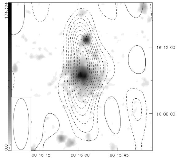
Figure 3: Low resolution RT map of the SZ effect in Cl 0016+16 (contours) superposed onto the Rosat PSPC image. The contours are -800, -720, -640, -560, -480, -400, -320, -240, -160, -80 and 80 $\mu$Jy. The restoring beam is $333\times 103^{\prime\prime}$ at an angle of $1.6^{\circ}$. The rms pixel noise on the map is $90~{}\mu$Jy. Only data from the shortest RT baselines ($<870~{}\lambda$) have been used in this map.

Figure 4: The Rosat PSPC image, our X-ray model, and the residuals from the fit. Contours are every 0.4 counts per $4^{\prime\prime}$ pixel.

Figure 5: Binned real part of the source-subtracted visibilities (filled points with error bars) for Cl 0016+16 observation against best fit model (open points joined by line).

Figure 6: Likelihood plot for values of $H_{0}$ from the fit of SZ decrement to the X-ray derived cluster model. The width of the plot indicates only the errors from the visibility data.

References

- [Biggs et al. 1999] Biggs A. D., Browne I. W. A., Helbig P., Koopmans L. V. E., Wilkinson P. N., Perley R. A.,1999, MNRAS, 304, 349.
- [Birkinshaw et al. 1984] Birkinshaw M., Gull S. F., Hardebeck H. E., 1984, Nat, 309, 34.
- [Birkinshaw & Hughes 1994] Birkinshaw M., Hughes J. P., 1994, ApJ, 420, 33.
- [Birkenshaw 1999] Birkinshaw M., 1999, Phys.Rept. 310, 97.
- [Baars et al. 1977] Baars J. W. M., Genzel R., Pauliny-Toth I. I. K., Witzel A., 1977, A&A, 61, 99.
- [Bridle et al. 2001] Bridle S. L., Zehavi I., Dekel A., Lahav O., Lasenby A. N., Hobson M. P., 2001, MNRAS, 321, 333.
- [Butcher & Oemler 1984] Butcher H., Oemler A., 1984, ApJ, 285, 426.
- [Carlstrom et al. 1996] Carlstrom J. E., Joy M., Grego L., 1996, ApJ, 456, L75.
- [Desert et al. 1998] Desert F.-X., Benoit A., Gaertner S., Bernard J.-P., Coron N., Delabrouille J., de Marcillac P., Giard M., Lamarre J.-M., Lefloch B., Puget J.-L., Sirbi A., 1998, New Astronomy, 3, p. 655.
- [Dressler & Gunn 1992] Dressler A., Gunn J. E., 1992, ApJS, 78, 1.
- [Fassnacht et al. 1999] C. D. Fassnacht, T. J. Pearson, A. C. S. Readhead, I. W. A. Browne, L. V. E. Koopmans, S. T. Myers , P. N. Wilkinson, 1999, ApJ, 527, 498.
- [Freedman et al. 2000] W. L. Freedman, B. F. Madore, B. K. Gibson, L. Ferrarese, D. D. Kelson, S. Sakai, J. R. Mould, R. C. Kennicutt, Jr., H. C. Ford, J. A. Graham, J. P. Huchra, S. M. G. Hughes, G. D. Illingworth, L. M. Macri, P. B. Stetson, 2000, ApJ in press.
- [Giovannini & Feretti 2000] Giovannini G., Feretti L., 2000 submitted to Elsevier Science.
- [Grainge et al. 1993] Grainge K., Jones M. E., Pooley G. G., Saunders R., Edge A., 1993, MNRAS, 265, L57.
- [Grainge et al. 1996] Grainge K., Jones M. E., Pooley G. G., Saunders R., Baker J., Haynes T., Edge A., MNRAS, 1996, 278, L17.
- [Grainge et al. 2001] Grainge K., Jones M. E., Saunders R., Pooley G. G., Edge A., Kneissl R., 2001, submitted to MNRAS.
- [Grainger et al. 2001] Grainger W. F., Das R., Grainge K., Jones M. E., Kneissl R., Pooley G. G., Saunders R., 2001, submitted to MNRAS.
- [Hanisch 1982] Hanisch, R., 1982, A&A 116, 137.
- [Henry et al. 1992] Henry J. P., Gioia I. M., Maccacaro T., Morris S. L., Stocke J. T., Wolter A., 1992, ApJ, 386, 408.
- [Hughes & Birkinshaw 1998] Hughes J. P., Birkinshaw M., 1998, ApJ, 501, 1.
- [Jones 1991] Jones, M. E., 1991 in Cornwell T.J., Perley R., eds, Proc. IAU Colloquium 131, Radio Interferometry: Theory, Techniques and Applications. Astonomical Society of the Pacific, 395.
- [Jones 1995] Jones M. E., 1995, Astrophys Lett & Comm, 32, 347.
- [Jones et al. 1993] Jones M. E., Saunders R., Alexander P., Birkinshaw M., Dillon N., Grainge K., Lasenby A., Lefebvre D., Pooley G. G., Scott P., Titterington D., Wilson D., 1993, Nat, 365, 320.
- [Jones and Saunders1996] Jones, M. E., Saunders R., 1996, in “Röntgenstrahlung from the Universe”, Eds Zimmermann H. U., Trümper J.E., Yorke M., 1996, MPE report 263.
- [Jones et al. 2001] Jones M. E., Edge A., Grainge K., Grainger W. F., Kneissl R., Pooley G. G., Saunders R., Miyoshi S.J., Tsuruta T., Yamashita K., Furuzawa A., Harada A., Hatsukade I., 2001, submitted to MNRAS.
- [Maggi et al. 2001] Maggi A. et al. in prep.
- [Mason et al. 2001] Mason B. S., Myers S. T., Readhead A. C. S., ApJL in press.
- [Moffet & Birkinshaw 1989] Moffet A. T., Birkinshaw M., 1989, ApJ, 98, 1148.
- [Neumann & Böhringer 1997] Neumann D. M., Böhringer H., 1997, MNRAS 289, 123.
- [Perlmutter et al. 1999] Perlmutter S. et al., 1999, ApJ, 517, 565.
- [Reese et al. 2000] Reese E. D. , Mohr J. J., Carlstrom J. E., Joy M. , Grego L., Holder G. P., Holzapfel W. L., Hughes J. P., Patel S. K., Donahue M., 2000, ApJ 533 38.
- [Roettiger, Burns & Loken 1993] Roettiger K., Burns J., Loken C., 1993, Ap. J., 407, L53.
- [Saunders 1995] Saunders, R., 1995, Astrophys Lett & Comm, 32, 339.
- [Smail et al. 1995] Smail I., Ellis R.S., Fitchett M. J., Edge A. C., 1995, MNRAS, 273, 277.
- [Sunyaev & Zel’dovich 1972] Sunyaev, R. A., Zel’dovich, Ya B., 1972, Comm. Astrophys. Sp. Phys., 4, 173.
- [Titterington 1991] Titterington D. J., 1991 in Cornwell T.J., Perley R., eds, Proc. IAU Colloquium 131, Radio Interferometry: Theory, Techniques and Applications. Astronomical Society of the Pacific.
- [Thompson et al. 1986] Thompson A., Moran J., Swenson G., 1986, “Interferometry and Synthesis in Radio Astronomy”, Kreiger Publishing Company, Malabar, Florida.
- [VLA calibration manual 1996] National Radio Astronomy Observatory, 1996, VLA calibration manual, NRAO, Charlottesville.