Inhomogeneous metal enrichment at $z\sim 1.9$: the Lyman limit systems in the spectrum of the HDF-S quasar

We present a detailed analysis of three metal absorption systems observed in the spectrum of the HDF-South quasar J2233-606 ($z_{\rm em}=2.238$), taking advantage of new VLT-UVES high resolution data ($R=45000$, S/N$=40-60$, $\lambda\lambda\,3050-10000$ Å). Three main components, spanning about 300 km s^-1, can be individuated in the Lyman limit system at $z\sim 1.92$. They show a surprisingly large variation in metallicities, respectively $\sim 1/500$, $1/8$ and $1/100$ solar. The large value found for the second component at $z\simeq 1.9259$, suggests that the line of sight crosses a star-forming region. In addition, there is a definite correlation between velocity position and ionisation state in this component, which we interpret as a possible signature of an expanding H ii region. The systems at $z\sim 1.94$ and $z\sim 1.87$ have also high metallicity, $\sim 1/4$ and $1/3$ solar. We find that photoionisation and collisional ionisation are equal alternatives to explain the high excitation phase revealed by O vi absorption, seen in these two systems. From the width of the Si iv, C iv, Si iii and C iii lines in the system at $z\sim 1.87$, we can estimate the temperature of the gas to be $\log T\raisebox{-5.0pt}{$\;\stackrel{{\scriptstyle\textstyle<}}{{\sim}}\;$}4.7$, excluding collisional ionisation. Finally, we compute the Si iv/C iv ratio for all Voigt profile components in a sample of $\log N$(C iv)$\raisebox{-5.0pt}{$\;\stackrel{{\scriptstyle\textstyle>}}{{\sim}}\;$}14$ systems at $z\raisebox{-5.0pt}{$\;\stackrel{{\scriptstyle\textstyle<}}{{\sim}}\;$}2$. The values show a dispersion of more than an order of magnitude and most of them are much larger than what is observed for weaker systems. This is probably an indication that high column density systems preferably originate in galactic halos and are mostly influenced by local ionising sources.

1 Introduction

High H i column density systems ($N$(H i) $\;\stackrel{{\scriptstyle\textstyle>}}{{\sim}}\;$ 10¹⁶ cm^-2) and especially Lyman limit systems ($N$(H i) $\;\stackrel{{\scriptstyle\textstyle>}}{{\sim}}\;$ 10¹⁷ cm^-2, hereafter LLS) arise in dense environments such as halos of large galaxies or the densest regions of filaments linking the galaxies (e.g. Katz et al. 1996; Gardner et al. 1997). Indeed, at redshifts $z\raisebox{-5.0pt}{$\;\stackrel{{\scriptstyle\textstyle<}}{{\sim}}\;$}1$, galaxies associated with LLS (detected by Mg ii absorption with equivalent width $w_{\rm r}$ $>$ 0.3 Å) are routinely identified revealing the presence of gaseous halos with radius larger than $\approx 40\ h^{-1}$ kpc (Bergeron & Boissé 1991; Steidel et al. 1994; Churchill et al. 1996; Guillemin & Bergeron 1997; Churchill et al. 2000a, b).

Although the ionisation corrections are large in LLS, the large number of associated metal lines can be used to constrain ionisation models and to estimate metallicity, ionisation state and abundances (e.g. Petitjean et al. 1992; Bergeron et al. 1994; Kirkman & Tytler 1999; Köhler et al. 1999; Prochaska & Burles 1999; Chen & Prochaska 2000).

In this paper, we present the study of three metal systems at redshifts $z_{\rm abs}\sim$ 1.87, 1.92, and 1.94 seen in the spectrum of the HDF-South quasar J2233-606 ($z_{\rm em}=2.238$, $B\simeq 17.5$; see Savaglio 1998; Savaglio et al. 1999). The systems are associated with a Lyman limit break observed at $\sim 2683$ Å (Sealey et al. 1998). Prochaska & Burles (1999, PB99) investigated the two systems at $z\sim 1.92$ and $z\sim 1.94$ in detail. They derived $\log N$(H i) $=17.15\pm 0.02$ and $16.33\pm 0.04$ at $z\sim 1.92$ and 1.94 respectively. They found the systems have solar abundance pattern, but significantly different metallicites: $\approx 1/50$ solar and less than $\approx 1/200$ solar for the two components at $z\sim 1.92$ and $\approx 40$ % solar at $z\sim 1.94$.

Here we take advantage of new complementary data of high resolution and high signal-to-noise ratio ($S/N$) to further constrain metallicity inhomogeneities in these systems. The paper is structured as follows: in Sect. 2 we report observational details and the line fitting procedure for the systems; in Sect. 3 we investigate the possible ionising mechanisms and the determination of metallicity and abundances. In Sect. 4, the observed behaviour of the ratio Si iv/C iv is described; finally, we report our conclusions in Sect. 5.

2 Comments on individual systems

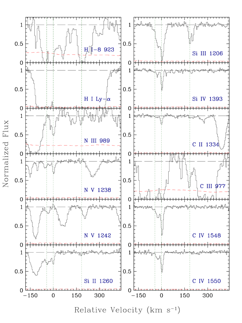
Figure 1: Main ionic transitions observed for the system at $z\sim 1.92$. The dotted lines mark the position of the clouds discussed in the text. From left to right: cloud 1 at $v\simeq-43$ km s^-1 ($z=1.9255$) with metallicity $\sim 1/500$ solar; cloud 2 at $v=0$ km s^-1 ($z=1.9259$) with metallicity $\sim 1/8$ solar and cloud 3 at $v\simeq+184$ km s^-1 ($z=1.92577$) with metallicity $\sim 1/100$ solar

Table 1: Ionic column densities for the $z\sim 1.92$ system. An (f) indicates that in the fit the parameter has been fixed to the value obtained for the previous absorption line

		$b$		$\log N$
Comp.	$z$	(km s-1)	Ion	(cm-2)
1…	1.92543a	$11\pm 5$	Si iv	$11.7\pm 0.2$
			Si iii	$11.2\pm 0.2$
			C iv	$12.2\pm 0.2$
2…	1.925719b	$14\pm 1$	Si iv	$12.23\pm 0.05$
			Si iii	$12.61\pm 0.04$
			C iv	$13.07\pm 0.03$
	(f)	(f)	N v	$<12.75\pm 0.08$
	(f)	(f)	N iii	$13.5\pm 0.2$
	1.925718b	$18\pm 11$	C ii	$12.4\pm 0.2$
3…	1.925950c	$7.6\pm 0.6$	Si ii	$12.26\pm 0.03$
			C ii	$12.91\pm 0.05$
			Mg ii	$11.72\pm 0.08$
	1.925989c	$6.7\pm 0.2$	Si iv	$12.72\pm 0.01$
			Si iii	$12.76\pm 0.09$
			C iv	$13.41\pm 0.01$
	(f)	(f)	N v	$<12.4\pm 0.1$
	(f)	(f)	N iii	$13.6\pm 0.2$
4…	1.927747c	$7.4\pm 0.8$	Si iii	$12.32\pm 0.03$
5…	1.927929c	$5.5\pm 0.8$	Si iii	$12.14\pm 0.04$

^a Error $30\times 10^{-6}$, ^b Error $7\times 10^{-6}$, ^c Error $4\times 10^{-6}$

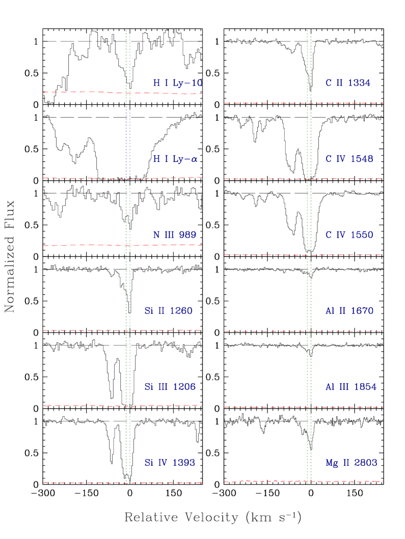
Figure 2: Main ionic transitions observed for the system at $z\sim 1.94$. The origin of the velocity axis is fixed at $z=1.942616$ and the dotted lines indicate the positions of components 7 and 8 in Table 2

Table 2: Ionic column densities for the $z\sim 1.94$ system

		$b$		$\log N$
Comp.	$z$	(km s-1)	Ion	(cm-2)
1…	1.94031a	$12\pm 1$	C iv	$12.67\pm 0.04$
	1.940258b	$19\pm 1$	O vi	$13.9\pm 0.1$
			H i	$13.28\pm 0.03$
2…	1.940730b	$7.0\pm 0.4$	C iv	$12.97\pm 0.02$
		$22\pm 3$	O vi	$13.9\pm 0.2$
			H i	$13.53\pm 0.07$
3…	1.941006b	$10\pm 1$	C iv	$12.78\pm 0.03$
	1.94107c	$22\pm 4$	O vi	$14.1\pm 0.1$
			H i	$13.2\pm 0.1$
4…	1.941791b	$5.8\pm 0.6$	C iv	$12.98\pm 0.05$
5…	1.941975b	$14.3\pm 0.7$	Si iv	$12.78\pm 0.03$
			Si iii	$12.70\pm 0.03$
	(f)	$16.4\pm 0.6$	C iv	$13.89\pm 0.01$
	1.94182c	$20\pm 4$	C ii	$12.9\pm 0.1$
	(f)	$91\pm 25$	H i	$13.80\pm 0.07$
6…	1.942001b	$3.7\pm 0.5$	Si iv	$12.66\pm 0.04$
			Si iii	$12.4\pm 0.1$
	(f)	$5\pm 1$	C iv	$12.84\pm 0.08$
	1.942011b	$9\pm 2$	C ii	$12.8\pm 0.1$
			Si ii	$11.79\pm 0.08$
	(f)	$23.9\pm 0.5$	H i	$15.60\pm 0.06$
7…	1.942429b	$10.3\pm 0.4$	Si iv	$13.34\pm 0.02$
			Si iii	$13.20\pm 0.04$
	(f)	(f)	N iii	$13.7\pm 0.1$
	(f)	$10.1\pm 0.4$	C iv	$14.01\pm 0.03$
	1.942484b	$17.1\pm 0.6$	C ii	$13.62\pm 0.02$
			Si ii	$12.59\pm 0.03$
			Mg ii	$12.54\pm 0.04$
			Al iii	$11.92\pm 0.05$
			Al ii	$11.39\pm 0.05$
	(f)	$26\pm 2$	H i	$16.1\pm 0.1$
8…	1.942618b	$9.1\pm 0.03$	Si iv	$13.39\pm 0.02$
			Si iii	$13.46\pm 0.05$
	(f)	(f)	N iii	$13.8\pm 0.1$
	(f)	$14\pm 1$	C iv	$14.1\pm 0.1$
	1.942614b	$5.2\pm 0.3$	C ii	$13.52\pm 0.03$
			Si ii	$12.53\pm 0.03$
			Mg ii	$12.37\pm 0.05$
			Al iii	$11.79\pm 0.05$
			Al ii	$11.21\pm 0.06$
	(f)	$15\pm 4$	H i	$15.8\pm 0.2$
9…	1.94269c	$18\pm 1$	C iv	$13.8\pm 0.2$

^a Error $11-20\times 10^{-6}$, ^b Error $\leq 10\times 10^{-6}$, ^c Error $>30\times 10^{-6}$

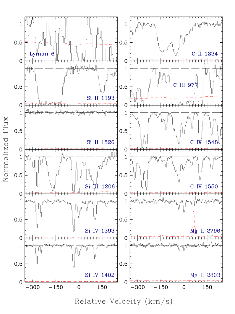
Figure 3: Main ionic transitions for the system at $z\sim 1.87$. The origin of the velocity axis is fixed at $z=1.87008$ corresponding to component 12 analysed in the text

New data on the HDF-South quasar have been obtained in October 1999 during the commissioning of UVES, the UV and Visual Echelle Spectrograph, mounted on the VLT Kueyen ESO telescope at Paranal (Chile). The spectrum is of high resolution ($R=45000$) and high signal-to-noise ratio ($S/N=40-60$ per resolution element) and covers the spectral range $\lambda\lambda\,3050-10000$ Å. The data reduction and spectrum analysis are reported in Cristiani & D’Odorico (2000). We use these data together with the echelle spectrum ($\lambda\lambda\,2275-3118$ Å) of high resolution ($R=30000$) obtained with the STIS instrument on board HST (Savaglio 1998).

When not otherwise stated, low-ionisation, weak lines of different species have been fitted together with the same number of sub-components, each with the same redshift and Doppler width. The same is true for high ionisation, complex and/or saturated lines. Absorption lines detected in the STIS spectrum (mainly N iii, C iii) are fitted using the same components used to fit Si iv. Voigt profile fitting is obtained in the context Lyman of MIDAS the ESO reduction package (Fontana & Ballester 1995).

2.1 The system at $z\sim 1.92$

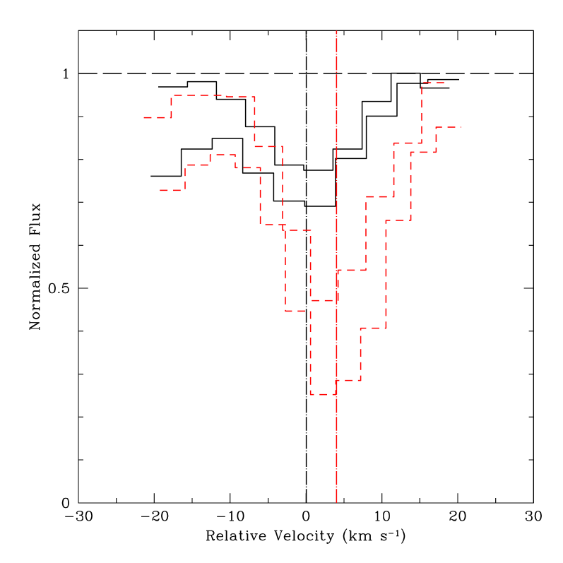
Figure 4: Superposition of the absorption lines due to Si ii $\lambda\,1260$, C ii $\lambda\,1334$ (solid line) at $z\simeq 1.92595$ and Si iv $\lambda\,1393$, C iv $\lambda\,1548$ (short-dashed line) at $z\simeq 1.92599$. The dot-dashed lines indicate the center of the two groups of lines separated by 4 km s^-1

The strong, well defined component at $z\simeq 1.92599$ (see Fig. 1 and Table 1) in the high-ionisation line profiles (C iv, Si iii, Si iv) is displaced by $4\pm 0.4$ km s^-1 with respect to the corresponding component at $z\simeq 1.92595$ seen in the low ionisation lines (C ii, Si ii) as shown in Fig. 4. The number of lines available together with the very good quality of the data give confidence that this shift is real. The simplicity of the velocity profiles suggests that this reflects the internal structure of an H ii region flow in which kinematics and ionisation state are well correlated (e.g. Henney & O’Dell 1999; Rauch et al. 1999).

The simultaneous fit of the H i Ly$\alpha$, Ly$\beta$, Ly$\epsilon$ and Ly-8 lines results in two main components at $z\simeq 1.92553$ and $z\simeq 1.92775$ with $\log N$(H i)$=17.1\pm 0.2$ and $16.7\pm 0.3$ respectively. Thus the two stronger H i absorptions are shifted relative to the main C ii and Si ii component observed at $z=1.92595$ by $\sim-43$ km s^-1 and $+184$ km s^-1 respectively. The mismatch in the velocity positions of the strongest H i  and C ii absorptions is apparent in Fig. 1, where the origin of the velocity axis is fixed at the position of the C ii absorption. The upper limit to the H i column density at the redshift of the main metal component is $\log N$(H i)$\raisebox{-5.0pt}{$\;\stackrel{{\scriptstyle\textstyle<}}{{\sim}}\;$}16$. This is derived by adopting the Doppler parameter as measured from the C ii line. It can be seen as well that at velocity position +184 km s^-1, the only metal transition detected is Si iii. The $3\,\sigma$ upper limit on the corresponding C iv absorption is $\log N$(C iv)$\raisebox{-5.0pt}{$\;\stackrel{{\scriptstyle\textstyle<}}{{\sim}}\;$}11.9$.

2.2 The system at $z\sim 1.94$

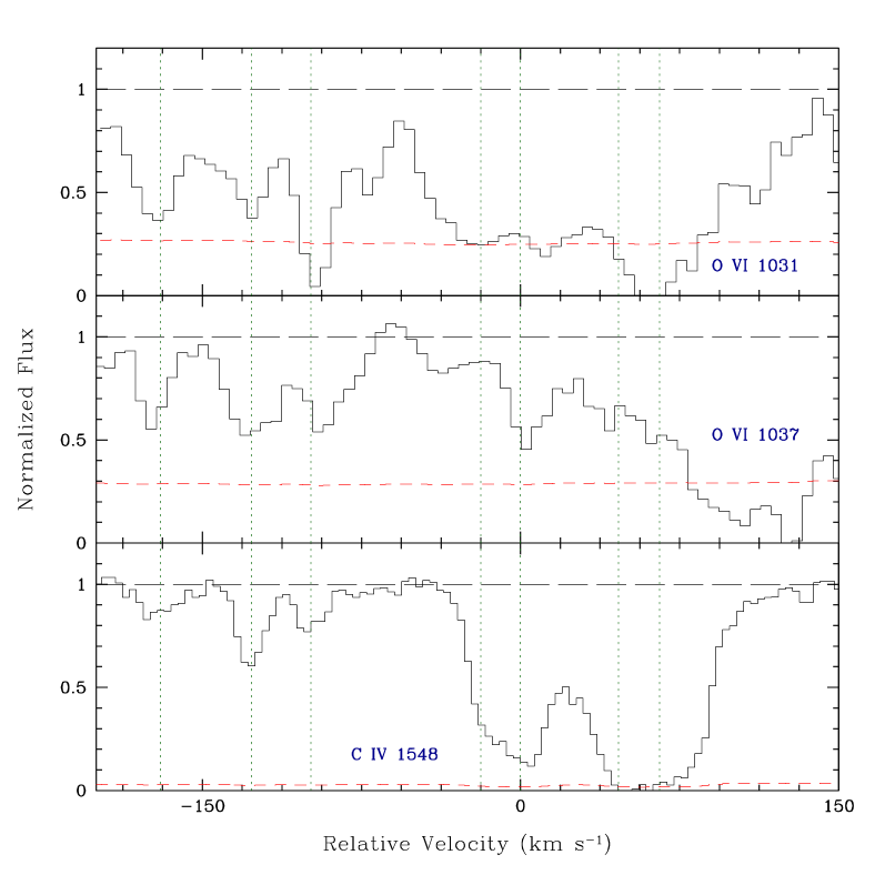
Figure 5: O vi $\lambda\lambda\,1031,1037$ for the system at $z\sim 1.94$. The velocity axis is centered at $z=1.941975$. The dotted lines show the position of the main components in C iv

Absorption profiles for this system are shown in Fig. 2.

Si iv and Si iii absorptions are fitted with the same components and Doppler parameters. C iv is saturated; we therefore fix the components at the redshifts determined for Si iv and then add weak components to reach a good fit. Si ii $\lambda\,1193,\ \lambda\,1260,\ \lambda\,1304,\ \lambda\,1526$, C ii $\lambda\,1334$, Mg ii $\lambda\,2803$, Al ii $\lambda\,1670$ and Al iii $\lambda\,1854$ are fitted together (same redshift and same Doppler parameter). Mg ii $\lambda\,2796$ is blended with a telluric absorption and is not considered in the fit. Results are given in Table 2. Most components shows significant differences in velocity (up to $\sim 25$ km s^-1) between high-ionisation and low-ionisation transitions, but blending is likely the main cause of this discrepancies.

Associated O vi is detected in the STIS portion of the spectrum (see Fig. 5). Although the $S/N$ ratio is not excellent, the O vi and C iv profiles are correlated with in particular three components (1, 2, 3 in Table 2) well detected in both species at $z\simeq$ 1.94026, 1.94073, 1.94107 ($v=-175$, $-127$ and $-92$ km s^-1respectively in Fig. 5).

The H i column densities quoted in Table 2 are obtained by fitting together H i Ly$\alpha$, Ly$\gamma$, Ly$\epsilon$, Ly-10, Ly-12 at the redshifts fixed by the C ii components. N v is not observed; the $3\,\sigma$ upper limit on the column density is $\log N$(N v)$\raisebox{-5.0pt}{$\;\stackrel{{\scriptstyle\textstyle<}}{{\sim}}\;$}12.15$.

2.3 The system at $z\sim 1.87$

This system has a complex structure spanning around 600 km s^-1, with 11 (16) components in Si iv (C iv). Mg ii is observed only at the redshift of the two central components (11 and 12 in Table 4). Unfortunately, important transitions like C ii $\lambda\,1334$, Si ii $\lambda\,1260$, Si iii $\lambda\,1206$ and C iii $\lambda\,977$ are badly affected by blending (see Fig. 3).

The Si iv doublet is fitted by itself and the redshifts of the components are used to fit Si iii. C iv is fitted by itself because more components with respect to Si iv are necessary to reach an acceptable fit. Table 4 displays the fitting parameters for the 17 components.

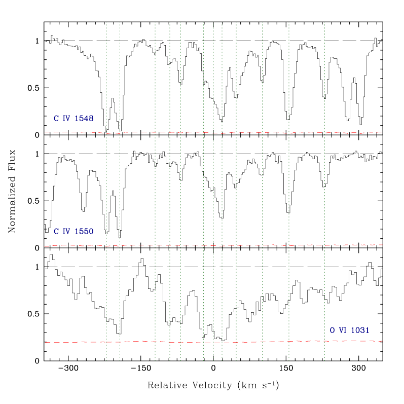
Figure 6: O vi $\lambda\lambda\,1031,1037$ for the system at $z\sim 1.87$. The velocity axis is centered at $z=1.8695$. The dotted lines show the position of the main components in C iv

Associated O vi is detected in the STIS portion of the spectrum (see Fig. 6), low $S/N$ ratio and partial blending with intervening H i lines prevent to carry on a best fit procedure in MIDAS. An indicative upper limit to the column densities in each component is estimated to be $\sim 13.7$ using the interactive fitting program Xvoigt (Mar & Bailey 1995). It is apparent from Fig. 6 that, although the C iv and O vi profiles are correlated, the distribution of the O vi phase is smoother than that of the C iv phase. N v is not detected: the $3\,\sigma$ limit on the column density is: $\log N$(N v)$<12.3$ for $z<1.87$ and $\log N$(N v)$<12.6$ for $z>1.87$.

Due to the heavy saturation of Ly$\alpha$ and Ly$\beta$ absorptions and to the complexity of the system, it is not possible to reliably constrain H i column densities for all the components. For components 2, 4 and 16 we estimate $\log N$(H i)$\simeq 15.2\pm 0.2$, $\simeq 14.9\pm 0.1$ and $\simeq 15.4\pm 0.1$ respectively from the simultaneous fit of H i Ly$\alpha$, Ly$\beta$, Ly$\gamma$, and Ly-6.

3 Ionisation models

The nature of the ionisation mechanisms is investigated comparing the observed column densities with those predicted by photoionisation models. For this we use the Cloudy software package (Ferland 1997) assuming ionisation equilibrium. In the models we adopt: (1) a total hydrogen density $n$(H)$=10^{-2.5}$ cm^-3, (2) a plane parallel geometry for the gas cloud, (3) the solar abundance pattern, and two ionising spectra (4a) the Haardt-Madau (Haardt & Madau 1996; Madau et al. 1999, hereafter HM) EUVB spectrum with galaxy contribution or (4b) a composite (hereafter SSP) of the spectrum produced by a simple stellar population with 20 % solar metallicity, age 0.1 Gyr (Charlot private communication) plus a power law, $f(\nu)\propto\nu^{-1}$, which increases the flux at energies greater than the He ii ionisation break (54.4 eV) by a factor of $\sim 3$ (Schaerer & de Koter 1997).

The ionisation parameter, $U$, defined by

$$U\equiv\frac{\phi_{912}}{cn_{\rm H}}=\frac{4\pi J_{912}}{hcn_{\rm H}}=2\times 10^{-5}\frac{J_{912}/10^{-21.5}}{n_{\rm H}/(1\mbox{cm}^{-3})}$$ (1)

(where $J_{912}$ is the intensity of the EUVB at 1 ryd) and the metallicity of the system are derived by matching the model output column densities with the observed values.

3.1 The system at $z\sim 1.92$

In Sect. 2.1 we have singled out three clouds at $z\simeq$ 1.9255, 1.9259, 1.9277 with $\log N$(H i) $\simeq 17.1$, $<$16, 16.7 respectively, corresponding to the $v=-43$ km s^-1 component which is the main component in H i (cloud 1), the $v=0$ km s^-1 component which is the main component in C ii and Si ii (cloud 2) and the $+184$ km s^-1 component which is detected in H i and Si iii only (cloud 3). At variance with PB99, we anlyse separately cloud 1 and cloud 2. As there is an uncertainty of $\sim 20$ km s^-1 on the redshift determination of cloud 1, we use for it the metal column densities of the slightly shifted component 2 at $z\simeq 1.92572$ (see Tab. 1). Thus, the metallicity we determine for this cloud could be an upper limit. Finally, the model for cloud 3 takes into account the possible Si iii absorption line (component 4 in Tab. 1) which was not observed by PB99.

Because of the large number of parameters (ionisation parameter, shape of the ionising flux, metallicities), the metallicity determination is most often degenerate. However, when the number of transitions is large and the column densities well determined, the mean metallicity and ionisation parameter can be estimated with reasonable uncertainties.

The observed column densities are reproduced by a SSP spectrum and a slight overabundance of silicon ([Si/H] $\sim 0.15$). The higher quality data allow us to reject the HM spectrum model which was considered viable in the analysis by PB99. Indeed, the observed column density pattern (C ii, C iv, Si ii, Si iii, Si iv) of cloud 2 is not reproduced by the HM spectrum for any combination of metallicity and ionisation parameter, even allowing for an over-solar abundance of silicon. Fig. 7 shows the predicted column densities as a function of $U$ for cloud 2 models. The column densities obtained in our best model are given in Table 3. The computed values for silicon ions can still be reconciled with the observed profiles. The discrepancy between observed and predicted N v and N iii column densities, discussed in PB99, is no longer present in our analysis. It is apparent from Fig. 7 that the Al ii column density is predicted larger than the upper limit derived from observations. This behaviour is even more apparent in Fig. 8 both for the column densities of Al iii and Al ii and for their ratio which is predicted $\sim 0.3$ dex lower than observed. The underabundance of aluminium observed in galactic low metallicity stars could reconcile the observed and computed results. On the other hand, magnesium does not seem to be overabundant as would be expected from the same halo star observations. Furthermore, the recombination coefficients used to compute the aluminium ionisation equilibrium are probably questionable as already noted by Petitjean et al. (1994).

For the other clouds, we derive that cloud 1 has similar ionisation parameter as cloud 2, $\log U\simeq-2.7$, $-2.8$. The metallicities of the two clouds differ by two order of magnitudes: [X/H] $\simeq-2.7$ and $-0.9$ respectively. The computation for cloud 3 is based solely on the Si iii column density and on the upper limits on the main transitions of silicon and carbon. The gas is probably in a low ionisation state, $-3.3\raisebox{-5.0pt}{$\;\stackrel{{\scriptstyle\textstyle<}}{{\sim}}\;$}\log U\raisebox{-5.0pt}{$\;\stackrel{{\scriptstyle\textstyle<}}{{\sim}}\;$}-3.1$, and has a low metallicity $-2.3\raisebox{-5.0pt}{$\;\stackrel{{\scriptstyle\textstyle<}}{{\sim}}\;$}$ [X/H] $\raisebox{-5.0pt}{$\;\stackrel{{\scriptstyle\textstyle<}}{{\sim}}\;$}-2.0$.

Figure 7: Ionic column densities computed by Cloudy (Ferland, 1997) for $\log N_{\rm HI}=16$, [X/H] $=-0.87$, [Si/H] $=0.15$ and an SSP ionising spectrum with 20 % solar metallicity (see text) vs. a modified ionisation parameter, $U$, as defined in the text. The symbols on the right side of the plot and the dashed orizontal lines indicate the observed column density values for cloud 2. The symbols sifhted to the right are upper limit measurements. The vertical dotted line indicates the best value of $U$ determined from the observed C iv, C ii, Si iv, Si iiiand Si ii column densities

Table 3: Observed and predicted ionic column densities for cloud 1 in the system at $z\sim 1.92$ (see text) and component 8 in the system at $z\sim 1.94$

	cloud 1 ($z\simeq 1.92595$)		comp. 8 ($z\simeq 1.942618$)
Ion	$\log N_{\rm obs}$	$\log N_{\rm pred}$	$\log N_{\rm obs}$	$\log N_{\rm pred}$
C ii	$12.91\pm 0.05$	12.94	$13.50\pm 0.03$	13.5
C iv	$13.41\pm 0.01$	13.41	$14.1\pm 0.1$	13.8
N iii	$13.6\pm 0.2$	13.48	$13.8\pm 0.1$	14.2
N v	$<12.4\pm 0.1$	11.55	$<12.15$	11.56
Mg ii	$11.72\pm 0.08$	11.67	$12.37\pm 0.05$	12.39
Al iii	$<11.19$	10.92	$11.79\pm 0.05$	12.09
Al ii	$<10.66$	11.25	$11.21\pm 0.06$	11.82
Si ii	$12.26\pm 0.03$	12.16	$12.59\pm 0.04$	12.59
Si iii	$12.8\pm 0.1$	13.1	$13.46\pm 0.05$	13.81
Si iv	$12.72\pm 0.01$	12.64	$13.39\pm 0.02$	13.39

From this we derive that most probably the three clouds are ionised by a local source of ionisation. This conclusion is strengthened by the observed correlation between kinematics and ionisation state in the component at $z\sim 1.9259$ (cloud 2). This together with the observations of variations in the metal content by about two orders of magnitude over a velocity interval of $\sim 50$ km s^-1, suggests that the line of sight crosses a region of intense star-formation activity. It would be most interesting to probe this by searching the field for emission line objects at this redshift.

3.2 The system at $z\sim 1.94$

Photoionisation models have been constructed for the two strong components 7 and 8 (see Table 2) both with $\log N$(H i) $\approx 16$. We have used as constraints the column densities of Si ii, C ii, and Si iv. We do not use C iv and Si iii because the lines are saturated.

Figure 8: Results from a series of Cloudy (Ferland, 1997) calculations assuming an overabundance [Si/H] $\simeq 0.2$, a metallicity [X/H]=-0.5, $\log N_{\rm HI}=15.8$ and an HM ionising spectrum including the contribution of galaxies. Plotted are the calculated ionic column densities vs. a modified ionisation parameter, $U$, as defined in the text. The symbols on the right side of the plot and the dashed orizontal lines indicate the observed column density values for the component of the metal system at $z=1.942614$, symbols shifted to the right give upper limit measurements. The vertical dotted line indicates the best value of $U$ determined from the observed C ii, Si iv and Si ii column densities

We cannot find any satisfactory fit to the data for a SSP ionising spectrum, except allowing for a Si/C ratio smaller than solar which is probably unreasonable. On the other hand, the HM spectrum accounts for the observed column densities in both components for $\log U\sim-2.3$ and $-0.7\raisebox{-5.0pt}{$\;\stackrel{{\scriptstyle\textstyle<}}{{\sim}}\;$}$ [X/H] $\raisebox{-5.0pt}{$\;\stackrel{{\scriptstyle\textstyle<}}{{\sim}}\;$}-0.5$. The uncertainty on the metallicity is mostly due to the uncertainty on the H i column density determination. The model requires also an overabundance of silicon, [Si/H] $\simeq 0.2$. In Fig. 8 the computed column densities for all the observed ions as a function of $U$ are reported in the case of component 8 and the values for the best fit parameters are in Table 3. It can be seen that most of the column densities are explained within a factor of two which is probably acceptable given the uncertainties on the column densities.

As previously noted, there is a discrepancy between the observed and computed Al ii and Al iii column densities. N iii is slightly overpredicted. Nitrogen could be underabundant which would not be surprising in the hypothesis of secondary origin of this element. A firm conclusion cannot be reached as the N iii column density is not well determined.

The three weak components 1, 2, and 3 show absorption due to O vi, C iv and H i. The observed ratios log (C iv/O vi), log (C iv/H i) are similar for the three components, average values are $\simeq-1.1\pm 0.2$ and $-0.5\pm 0.1$ respectively. We investigate both the possibilities of photo- or collisional ionisation.

The two adopted ionising spectra can reproduce the observed column density pattern in the context of photoionisation. But N v  is always overpredicted: $\log N$(N v)$\sim 13$ instead of $<$12.15 (3$\sigma$) as observed. In the case of the HM spectrum the parameters vary in the ranges $-0.15\raisebox{-5.0pt}{$\;\stackrel{{\scriptstyle\textstyle<}}{{\sim}}\;$}\log U\raisebox{-5.0pt}{$\;\stackrel{{\scriptstyle\textstyle<}}{{\sim}}\;$}0.2$ and $-1.4\raisebox{-5.0pt}{$\;\stackrel{{\scriptstyle\textstyle<}}{{\sim}}\;$}$ [X/H] $\raisebox{-5.0pt}{$\;\stackrel{{\scriptstyle\textstyle<}}{{\sim}}\;$}-1.1$ for the three components. While for the SSP spectrum $-0.86\raisebox{-5.0pt}{$\;\stackrel{{\scriptstyle\textstyle<}}{{\sim}}\;$}\log U\raisebox{-5.0pt}{$\;\stackrel{{\scriptstyle\textstyle<}}{{\sim}}\;$}-0.55$ and $-0.52\raisebox{-5.0pt}{$\;\stackrel{{\scriptstyle\textstyle<}}{{\sim}}\;$}$ [X/H] $\raisebox{-5.0pt}{$\;\stackrel{{\scriptstyle\textstyle<}}{{\sim}}\;$}-0.22$.

In the hypothesis of collisional ionisation, the observed column density ratio log (C iv/O vi) is consistent with a temperature $\log T=5.35$ (Sutherland & Dopita 1993). The prediction for the other ratios are: log (C iv/H i)$\simeq-0.03$, log (O vi/H i)$\simeq 1.30$ for solar metallicities. In order to match the observed ratios, the metallicity should be decreased to $\sim 1/3$ solar. Thus, if we assume collisional ionisation for these components and a solar abundance pattern, we get a metallicity comparable to the one predicted by Cloudy with the SSP spectrum. At this temperature, collisional ionisation predicts also: log (N v/C iv)$\sim 0.6$ while $-0.5$ is observed. Therefore in the framework of these models, N v observations can be explained only if nitrogen is deficient by an order of magnitude compared to carbon.

In conclusion, the gas in this system is likely of quite high metallicity (larger than 0.1 solar) for this redshift. The ionisation state can be explained by photoionisation by a HM type spectrum. In this case however, metallicity is three times less in the high-ionisation phase (components 1, 2 and 3) compared to the low-ionisation phase (components 7 and 8). The model can be reconciled with similar metallicities in both phases in case the high ionisation phase is predominantly ionised by a local source of photons or if it is collisionally ionised.

Both the photo- and collisional ionisation models predict that nitrogen is underabundant with respect to solar [N/C]$\raisebox{-5.0pt}{$\;\stackrel{{\scriptstyle\textstyle<}}{{\sim}}\;$}-0.5$.

3.3 The system at $z\sim 1.87$

We first determine an upper limit on the temperature of the gas from the measured Doppler parameter, in the hypothesis of pure thermal broadening. We choose three narrow, resolved components (2, 4 and 17; see Table 4 and Fig. 3) with detected Si iv, Si iii, C iv and, the last one, C iii absorptions; the observed Doppler parameter are consistent with a temperature $\log T<4.7$. In the hypothesis of collisional ionisation, at this temperature most of the carbon would be in C ii and C iii ions, O vi would not be present, and silicon would be mainly in Si iii and Si iv. From the ionic fractions calculated by Sutherland & Dopita (1993), at $\log T=4.6$ $\log$ (Si iii/Si iv) $\simeq 0.8$, and at $\log T=4.8$ $\log$ (Si iii/Si iv) $\simeq 0.16$ and $\log$ (C iii/C iv)$\simeq 1.74$. This excludes the possibility that the gas phase giving rise to the observed silicon and carbon transitions is collisionally ionised.

However, O vi could still arise from a collisionally ionised phase. Indeed, the co-existence of these two ionising mechanisms has been explained by e.g. the presence of a tail of shock-heated gas at high temperature away from the curve of equilibrium (Haehnelt et al. 1996) or a two phase halo where clouds photoionised by the EUVB at an equilibrium temperature of $\sim 10^{4}$ K and giving origin to the relatively narrow lines of C iv, Si iv, etc., are in pressure equilibrium with the hotter halo gas in which O vi arises (Petitjean et al. 1992; Mo & Miralda-Escudé 1996). The latter scenario predicts broad, shallow absorption for O vi and C iv originating in the hot gas. The low $S/N$ ratio STIS spectrum marginally shows that these lines are not as broad as those observed e.g. by Kirkman & Tytler (1999).

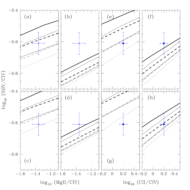
Figure 9: Results from a series of Cloudy calculations (Ferland, 1997). Curves represents Si iv/C iv column density ratio vs. Mg ii/C iv (panels a-d) and C ii/C iv (panels e-h) ratio as the ionisation parameter varies in the range $-4<\log U<-1$. Different curves are for $\log N$(H i)$=15$ (thin lines) and $\log N$(H i)$=17$ (thick lines), [X/H] $=-0.5$ (solid lines), [X/H] $=-1$ (dashed lines), and [X/H] $=-1.5$ (dotted lines). The panels have different ionising spectra and silicon abudances: a,e HM ionising spectrum and solar abundance pattern; b,f SSP spectrum and solar abundance pattern; c,g HM ionising spectrum and [Si/H] $=0.1$; d,h SSP spectrum and [Si/H] $=0.1$ The superposed points are the observed Mg ii/C iv and C ii/C iv column density ratios for component 12 of the system at $z\sim 1.87$

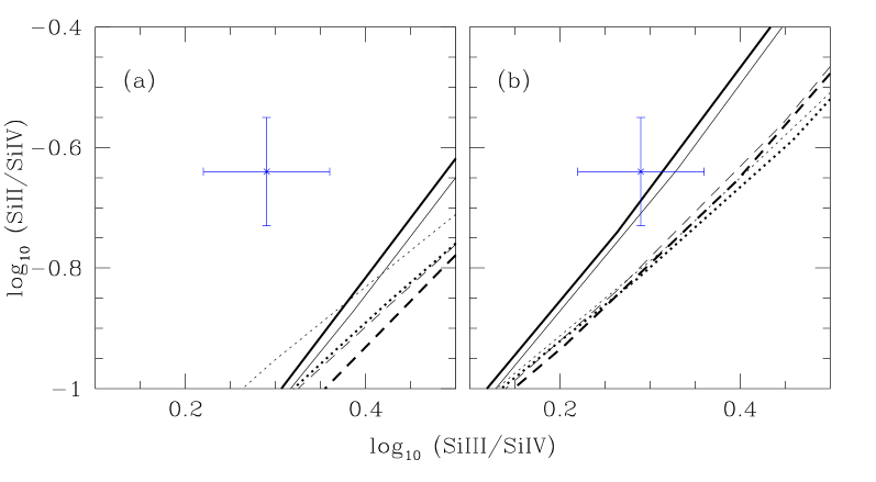
Figure 10: Results from a series of Cloudy calculations (Ferland, 1997). Curves represent Si ii/Si iv vs. Si iii/Si iv column density ratio as the ionisation parameter varies in the range $-4<\log U<-1$. The different curves describe the same models as in Fig. 9 for an HM ionising spectrum (panel a) and an SSP spectrum (panel b). The superposed point is the corresponding observed ratio

The high uncertainty in the H i column density for most of the components and the blending of many interesting absorption lines (refer to Sect. 2.3) makes an abundance analysis for this system difficult. A fit to the column densities in component 2, at $z\simeq 1.8675$, shows that the SSP spectrum model is best suited with $\log U\simeq-2.36\pm 0.04$, [X/H] $\simeq-0.4\pm 0.1$ and an overabundance of silicon, [Si/H] $\simeq 0.1$.

In the case of component 12 at $z\simeq 1.87008$ for which we do not have a reliable determination of H i column density, we run a grid of photoionisation models varying the main parameters. On the basis of what is found from the previous modelisation, we consider metallicities between $\sim 1/3$ and $\sim 1/30$ solar, solar abundance pattern or an overabundance of silicon, [Si/H] $=0.1$. Fig. 9 shows the predicted Si iv/C iv ratio as a function of Mg ii/C iv and C ii/C iv ratios for the ionising parameter varying between $-4<\log U<-1$. Observed ratios are shown as black points. Three models are consistent with the data: an HM ionising spectrum with solar abundance pattern and metallicity [X/H] $\sim-1$ for $\log N$(H i)$=15$ or [X/H] $=-1.5$ for $\log N$(H i)$=17$ (panels a,e); an HM ionising spectrum with overabundance of silicon, $\log N$(H i)$=15$ and metallicity [X/H] $=-1.5$ (panels c, h); an SSP spectrum with overabundance of silicon and a metallicity [X/H] $\sim-0.5$ (panels d, g). The Si iii/Si iv vs. Si ii/Si iv plot favour the latter model (see Fig. 10).

In conclusion, we find that the two components at $z\simeq 1.8675$ and at $z\simeq 1.87008$ can be explained by a model with a local ionising stellar source and a gas metallicity of $\sim 1/3$ solar.

4 The Si iv/C iv ratio

It is well known that the Si iv/C iv  ratio in high-ionisation systems depends critically on the strength of the He ii ionisation edge (54 eV) break. Direct observations of the He ii Ly$\alpha$ absorption in QSO spectra (Jakobsen et al. 1994; Davidsen et al. 1996; Hogan et al. 1997; Reimers et al. 1997; Zheng et al. 1998) show a marked decrease of the opacity for $z<3$. Detailed investigation of the Si iv/C iv ratio have been carried out by Songaila & Cowie (1996); Savaglio et al. (1997); Giroux & Shull (1997) and Songaila (1998) among others. They all agree on the fact that the above ratio increases strongly between $z=2$ and $z=4$ with a possible discontinuity around $z=3$. In particular, Songaila (1998) collected a sample of C iv systems with $N$(C iv)$>5\times 10^{12}$ cm^-2, and obtained median values of $0.043^{+0.015}_{-0.008}$ for all the systems below $z=3$, and $0.15\pm 0.04$ above $z=3$ (errors are $1\,\sigma$ computed using the median sign method). Boksenberg (1998) questioned this result, based on an analysis of the redshift evolution of the ion ratios in individual Voigt components within complex systems.

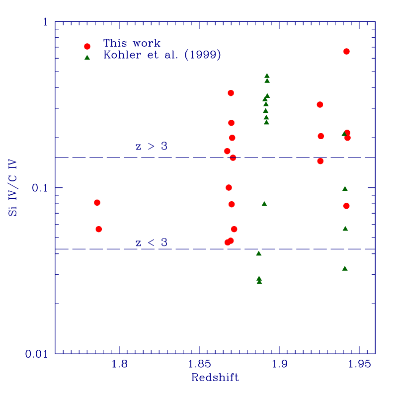
Figure 11: The values of the Si iv/C iv column density ratio for the single components of the metal systems in our sample (see text) are reported as a function of redshift. The two long-dashed lines are the median values computed by Songaila (1998) from lines in her sample below and above $z=3$

The Si iv/C iv ratios for the individual components of the three considered systems are plotted as a function of redshift in Fig. 11 together with the data by Köhler et al. (1999) who observed 4 systems at similar resolution. All systems have $z<3$. Data are spread over more than an order of magnitude and most of them are above the value estimated by Songaila (1998) for systems with $z<3$. It has to be noted that all but one of the systems in our sample have total C iv column density $>10^{14}$ cm^-2, while only 10 % of Songaila’s systems at $z<3$ belongs to this range of column densities.

As a comparison, we consider the HST data on absorption lines arising in the Milky Way halo gas (Savage et al. 2000). The observed Si iv and C iv transitions are weak, thus we transform the observed equivalent width in column density by using the curve of growth relationship for optically thin gas. The weighted mean of the 9 obtained estimates (corresponding to different lines of sight) is Si iv/C iv $\simeq 0.413\pm 0.009$ and the values are spread between $\sim 0.1$ and $\sim 0.6$.

This result supports the idea that high column density systems, which most probably arise in halos of galaxies, have higher values of the Si iv/C iv ratio compared to weak systems arising in regions more typical of the intergalactic medium. The systems studied here are probably influenced by local ionising sources rather than by the diffuse UV background.

5 Conclusion

We have discussed the nature of the three prominent metal absorption systems observed in the UVES spectrum of the HDF-South quasar J2233-606.

We analyse the velocity structure of the systems and their ionisation and abundance properties mainly by means of photoionisation models performed with the Cloudy software package (Ferland 1997). The main conclusions we draw are the following:

1. - The signature of a probable expanding flow in an H ii region is observed in the main metal component of the Lyman limit system, at $z\simeq 1.9259$, which shows a correlation between ionisation state and kinematics. Furthermore, the two main components in the H i absorption profile are shifted by $-43$ km s^-1 and $+184$ km s^-1 with respect to that component. The observed column density pattern is explained by a photoionisation model with a local stellar source and three different metallicities, $\sim 1/500$ and $\sim 1/100$ solar for the two H i clouds and $\sim 1/8$ solar for the metal component. The high metallicity in the latter cloud and the marked inhomogeneity suggest that the line of sight intersects a region of ongoing star formation and recent metal enrichment.

2. - The system at $z\sim 1.94$ shows high metallicity, $\sim 1/4$ solar, when modelled with photoionisation by an HM spectrum. There are three components at higher ionisation where strong O vi absorption is detected. The metallicity of these components is lower or equal to the one in the low ionisation components depending if the same or a different ionising source (SSP spectrum or collisional) is considered. Al ii and Al iii are badly underestimated by the model, this could be due to a still low accuracy in the recombination coefficients for this element (Petitjean et al. 1994).

3. - The system at $z\sim 1.87$ shows associated O vi absorptions. The same ionisation origin for these lines and the narrow transitions of C iv, Si iv,Si iii, etc, is excluded, thus a more complex scenario has to be taken into account. In order to test the different explanations which have been proposed it will be interesting to obtain spectra at high resolution and signal-to-noise ratio of the O vi complexes. We could investigate only two of the 17 components, both agree with [X/H] $\sim 1/3$ solar and a local stellar ionising source.

4. - The analysis of the Si iv/C iv column density ratio for a sample of systems at $z\raisebox{-5.0pt}{$\;\stackrel{{\scriptstyle\textstyle<}}{{\sim}}\;$}2$ with total $N$(C iv)$>10^{1}4$ cm^-2, shows a ditribution skewed towards higher values than observed by Songaila (1998). A comparison with analogous results for the gas in the halo of our galaxy implies that higher total C iv column density systems present higher values of the ratio Si iv/C iv, likely because they arise in a galactic environment and are influenced by local ionising sources rather than by the UV background.

Table 4: Ionic column densities for the $z\sim 1.87$ system

		$b$		$\log N$
Comp.	$z$	(km s-1)	Ion	(cm-2)
1…	1.86733c	$60\pm 6$	C iv	$13.31\pm 0.09$
2…	1.867494a	$5.3\pm 0.2$	Si iv	$12.97\pm 0.01$
	(f)	$5.2\pm 0.4$	Si iii	$12.65\pm 0.03$
	(f)	(f)	Si ii	$11.7\pm 0.1$
	(f)	(f)	C ii	$12.4\pm 0.1$
		$5.9\pm 0.3$	C iv	$13.75\pm 0.02$
3…	1.86756b	$25\pm 2$	C iv	$13.63\pm 0.05$
4…	1.867748a	$4.6\pm 0.4$	Si iv	$12.49\pm 0.02$
		$5\pm 1$	Si iii	$11.93\pm 0.05$
	1.867758a	$6.\pm 0.3$	C iv	$13.82\pm 0.02$
5…	1.867980b	$1.5\pm 0.7$	C iv	$12.\pm 0.2$
6…	1.868459b	$3\pm 3$	Si iv	$11.6\pm 0.1$
		$9\pm 2$	C iv	$12.56\pm 0.05$
7…	1.868749b	$7.8\pm 0.9$	C iv	$12.77\pm 0.04$
8…	1.868966a	$8.4\pm 0.5$	C iv	$13.12\pm 0.02$
9…	1.869414a	$1.5\pm 0.8$	C iv	$12.5\pm 0.2$
10…	1.86964c	$23\pm 4$	Si iv	$12.3\pm 0.1$
		$18\pm 1$	C iv	$13.62\pm 0.04$
11…	1.869767a	$6.6\pm 0.2$	Si iv	$13.12\pm 0.02$
	(f)	$8.4\pm 0.5$	Si iii	$13.09\pm 0.05$
	1.869756b	$8\pm 1$	Mg ii	$11.91\pm 0.04$
			Al ii	$11.1\pm 0.1$
			Al iii	$<11.48\pm 0.09$
	1.869779a	$7.7\pm 0.5$	C iv	$13.55\pm 0.04$
12…	1.870075a	$8.3\pm 0.6$	Si iv	$12.72\pm 0.02$
	(f)	$6.5\pm 0.5$	Si iii	$13.01\pm 0.07$
	1.870086a	$4.8\pm 0.6$	Si ii	$12.08\pm 0.09$
			Mg ii	$11.97\pm 0.03$
			Al ii	$11\pm 0.1$
			Al iii	$<11.2\pm 0.1$
		$10\pm 2$	C ii	$13.53\pm 0.04$
	1.870061a	$12\pm 1$	C iv	$13.33\pm 0.07$
13…	1.870232b	$4\pm 1$	Si iv	$12.01\pm 0.08$
	(f)	$6\pm 1$	Si iii	$12.13\pm 0.06$
		$33\pm 6$	C iv	$13.1\pm 0.1$
14…	1.870411b	$3\pm 2$	Si iv	$11.6\pm 0.1$
	(f)	$5\pm 1$	Si iii	$11.7\pm 0.1$
15…	1.870582a	$4.2\pm 0.5$	Si iv	$12.24\pm 0.03$
	(f)		Si iii	$12.17\pm 0.07$
		$6.1\pm 0.7$	C iv	$12.94\pm 0.05$
16…	1.871079a	$8.6\pm 0.2$	Si iv	$12.86\pm 0.01$
	(f)		Si iii	$12.64\pm 0.07$
	(f)	$6.6\pm 0.8$	C iii	$15.9\pm 0.5$
	1.871102a	$10.2\pm 0.2$	C iv	$13.68\pm 0.01$
17…	1.871796b	$6\pm 1$	Si iv	$12.03\pm 0.05$
	(f)		Si iii	$11.6\pm 0.1$
	(f)	$11\pm 3$	C iii	$13.1\pm 0.1$
	1.871808a	$8.5\pm 0.3$	C iv	$13.28\pm 0.01$

^a Error $\leq 5\times 10^{-6}$, ^b Error $6\div 15\times 10^{-6}$, ^c Error $\geq 50\times 10^{-6}$