A maximum-likelihood approach to removing radio sources from SZ observations, with application to Abell 611

Abstract

We describe a maximum-likelihood technique for the removal of contaminating radio sources from interferometric observations of the Sunyaev-Zel’dovich (SZ) effect. This technique, based on a simultaneous fit for the radio sources and extended SZ emission, is also compared to techniques previously applied to Ryle Telescope observations and is found to be robust. The technique is then applied to new observations of the cluster Abell 611, and a decrement of $-540\pm 125$ $\mu$Jy beam^-1 is found. This is combined with a ROSAT HRI image and a published ASCA temperature to give an $H_{0}$ estimate of $52^{+24}_{-16}$ km s^-1 Mpc^-1.

1 Introduction

This paper is concerned with the subtraction of radio sources which would otherwise contaminate or obliterate detections of the Sunyaev-Zel’dovich (SZ) effect [1970, 1972] towards galaxy clusters. The work described here is in connection with the Ryle Telescope (RT, see e.g. Jones et al. 2001 and Grainge et al. 2001b), but the issues are relevant to all cm-wavelength SZ observations with interferometers (see e.g. Reese et al. 2000). For a massive cluster at moderate or high redshift, the flux that the RT detects from the SZ effect at 15 GHz is typically $-$500 $\mu$Jy on its shortest baselines. This is sufficiently faint that radio sources will almost invariably be present with comparable or greater amplitudes. Thus removing the effects of radio sources is an essential step. We describe and compare two past methods of measuring SZ decrements in the presence of sources as well as a maximum-likelihood method. We then apply this to new RT observations of cluster A611 which we combine with X-ray data to estimate $H_{0}$. All coordinates are J2000 and, except where otherwise stated, we use an Einstein-de-Sitter world model.

2 Removing radio sources from SZ observations with the RT

As the RT is an interferometer with a wide range of baselines, it can simultaneously measure the extended SZ flux and the fluxes and positions of the small angular size radio sources. Figure 1 illustrates the variation of SZ flux with baseline for the RT when observing a massive Abell cluster at $z=0.171$. The variation with redshift is slight over the range $z=0.15$–$5$, as shown in Grainge et al. [2001b]. The SZ effect has effectively been completely resolved out for baselines above $\simeq 1.5$ k$\lambda$, and so these “long” baselines can be used to measure sources and so remove their effects from the SZ signal seen on the “short” baselines. The measurements are simultaneous and, of course, at the same frequency, and so the spectral index is unimportant. Variability is unimportant if the telescope configuration does not change; see Grainge et al. [1996] for details. By choosing an interferometer configuration such that there are more long baselines than short, it is possible to optimise the observations to achieve good signal-to-noise for the SZ effect without it being dominated by noise from unsubtracted sources.

Figure 1: The flux density as a function of baseline for a spherical King-model cluster with central electron density $=10^{4}{\rm m}^{-3},\beta=0.65,\mbox{core radius}=60\hbox{${}^{\prime\prime}$}$, $T_{e}=7.8\times 10^{7}~{}\mbox{K}$, $z=0.171$ and $H_{0}$=50 km s^-1 Mpc^-1, as observed with the RT. (From Grainge 1996). The shortest RT physical baselines are 870 $\lambda$; this becomes somewhat shorter with projection.

There are three methods of source subtraction that have been applied to RT data:

1. using Clean, which has been used for the bulk of published SZ measurements from the RT (e.g. Grainge et al. 1996);

2. the matrix method, which was first used by Grainge [1996]; and

3. the FluxFitter method, first used by Das [1999], and used here in modified form.

This sequence began with Clean, the classical radio-astronomy image deconvolution technique (see e.g. Greisen 1994 and Perley et al. 1989). The matrix method is a linear method for removing the effects of sidelobes, and FluxFitter – using maximum likelihood – addresses the problem of simultaneously fitting both radio sources and SZ decrement.

2.1 The test data

The three methods can be explained and compared with an example of a simulated dataset containing both sources and an SZ effect. The simulation is of a 54 $\times$ 12-hour long observation of a field at declination $44^{\circ}$. The $uv$ coverage is based on a standard Cb configuration for the RT; in this configuration four aerials are parked on an east-west rail-track at locations 36, 72, 90 and 108 m from the closest fixed aerial (see Grainge et al. 1996 for details). The point-source fluxes and positions are shown in Table 1, and the noise level was set to 7 mJy visibility^-1/2, corresponding to 200 $\mu$Jy day^-1/2, as expected for a standard RT observation with five aerials. The SZ decrement is based on Abell 2218, and is modelled as an isothermal ellipsoid with a King electron density profile [1972] at the centre of the map with a central electron density of $10^{4}{\rm m}^{-3}$, $\beta=0.65$, a temperature of $8.7\times 10^{7}$ K and core radii of 60^′′ and 40^′′ on the sky and 49^′′ ($=\sqrt{60\times 40}$) along the line of sight. The central temperature decrement for this cluster is 0.82 mK and, as observed with the RT, the cluster gives $-$660 $\mu$Jy beam^-1 on the shortest baseline.

Table 1: The source fluxes and positions in the simulated data set. The convention used in this and other tables is: positive $\Delta$RA is an increase in the RA value, so the source is to the East (to the left on conventional maps) and positive $\Delta$Dec is an increase in Dec, i.e. to the North.

Source number	Flux	Offset from pointing centre
	($\mu$Jy beam-1)	(arcseconds)
1	2960	$-$10, 10
2	910	35, 15
3	255	$-$50, $-$40
4	170	$-$120, 100
5	100	0, 0
6	80	60, $-$60

2.2 The CLEAN method

For this method, a dirty (i.e. unCleaned) map of all the baselines longer than 1.5 k$\lambda$ is produced within Aips [1994]. Natural weighting is used to give the best possible signal-to-noise ratio at the expense of larger sidelobes. The map is Cleaned in the standard way by placing Clean boxes around the obvious sources. After deconvolution, the source fluxes are measured, using the Aips verb Maxfit, which interpolates the position and value of the maximum flux density. The measured fluxes are then removed from the visibility data using the task Uvsub.

The sources and the positions found in the simulated dataset are listed in Table 2, and the Cleaned map is shown in Figure 2. The noise in the map due to the system temperature is 38 $\mu$Jy beam^-1. The six model sources are labelled; note that only four brightest were found.

A map made with baselines longer than 1.5 k$\lambda$ was consistent with noise after these four sources had been subtracted. The SZ flux observed was $-675\pm 72$ mJy beam^-1, at a position ($-4$, $-2$) arcsec from the pointing centre. The SZ values were measured with Maxfit from a map made with the baselines shorter than 1.0 k$\lambda$.

Table 2: Fluxes and positions as measured by Maxfit after Cleaning with four Clean boxes. The noise on each flux is 38 $\mu$Jy.

Source number	Flux	Offset from pointing centre
	($\mu$Jy beam-1)	(arcseconds)
1	3040	$-$9.6, 9.6
2	970	34.5, 15.8
3	270	$-$49.9, $-$45.8
4	170	$-$120.1, 91.9

Table 3: Fluxes and positions from the Clean method with six Clean boxes.

Source number	Flux	Offset from pointing centre
	($\mu$Jy beam-1)	(arcseconds)
1	3020	$-$9.6, 9.5
2	950	34.5, 15.8
3	240	$-$47.6, $-$42.0
4	180	$-$121.6, 98.4
5	85	12,$-$7
6	82	70,$-$70

Figure 2: A Cleaned map of the simulated data made with baselines longer than 1.5 k$\lambda$. Source 1 has had 2500$\mu$Jy beam^-1 of flux already removed to aid identification of weaker sources. The contour levels are $-$55$\times$(1, $\surd{2}$, 2) $\mu$Jy beam^-1 (dashed), 55$\times$(1, $\surd{2}$, 2, $\surd{8}$, 4, …) $\mu$Jy beam^-1 (solid). The beamsize FWHM (45^′′ $\times$ 26^′′ at 4^∘) is shown in the bottom left. The noise in the map due to the system temperature is 38 $\mu$Jy beam^-1.

A comparison of the sources found (Table 2) and the sources actually in the model (Table 1) shows the how well the Clean method works. The most glaring problem is that only four out of the original six sources have been detected. As lower-frequency surveys such as FIRST, NVSS or optical images often provide information about the source envirnoment at 15 GHz, the long-baseline map is rarely used in isolation. As such, a second test was performed, placing the Clean boxes as before, but adding small Clean boxes around the locations of the other two weaker sources. The positions and fluxes of the six sources are shown in Table 3. The noise on the long-baseline map is 38 $\mu$Jy beam^-1. Thus additional radio or optical information leads to the detection of the two faintest sources.

2.2.1 Source finding

Source finding is done in a non-linear, iterative manner. A typical source-subtraction process may involve many iterations of map making, running the subtraction algorithm on the sources found, mapping residuals, finding another source and then adding that into the model.

A high signal-to-noise source is easy to identify, and causes no problems. However, the process becomes subjective around signal-to-noise ratios of 4 to 3.5. This is the point at which the non-Gaussian, correlated statistics in the image plane conspire with the high RT sidelobes (when using a few antennas for source finding) to make source identification more difficult.

Radio sources in the clusters we observe have angular sizes smaller than the maximum resolution used. However, the number of Clean components is generally much larger than the number of sources in the field. With the test data, only four sources were identified, but Aips produced a model with 28 Clean components. Since the real sources are evidently point sources, this is over-modelling the data; and potentially biasing. There is also a degree of subjectivity in the placing and sizing of Clean boxes.

2.3 The matrix method

The matrix method was initally developed by KG [1996], and we here describe it and assess its performance. In the matrix method, sources are first identified from a unCleaned long-baseline map, and Maxfit used to measure the positions and the fluxes of the sources. The convolution that occurs when observing with an interferometer means that the flux on the dirty map of the $j^{\rm th}$ source, $S_{\mathrm{dirty},j}$, is given by

$$S_{\mathrm{dirty},j}=\sum_{i=1}^{n}S_{{\rm sky},i}\,B_{i,j}\,P_{i},$$ (1)

where $S_{{\rm sky},i}$ is the true flux on the sky of the $i^{th}$ point source, $B_{i,j}$ is a factor due to the synthesised beam that depends on the displacement (on the sky) between the source in question and the $i^{th}$ source, and $P_{i}$ is the primary (envelope) beam attenuation. The value of $B_{i,j}$ is directly measured from the dirty beam produced by Horus. There is thus a matrix equation linking the measured dirty fluxes with the true sky fluxes, which is solved by inverting the matrix. This method has the advantage over Clean in that sources that are measured in the map to be point sources are modelled with one flux and position. With the simulated test data, the four sources identified with the Clean method were used. The resulting matrix was

$$\left(\begin{array}[]{c}2875\\ 473\\ 105\\ 585\\ \end{array}\right)=\left(\begin{array}[]{cccc}1&0.13&-0.03&0.16\\ -0.13&1&0.02&-0.04\\ -0.03&0.02&1&0.12\\ 0.16&-0.04&0.12&1\\ \end{array}\right)\left(\begin{array}[]{c}S_{{\rm sky},1}\\ S_{\mathrm{sky},2}\\ S_{\mathrm{sky},3}\\ S_{\mathrm{sky},4}\\ \end{array}\right),$$ (2)

where the vector on the left side of the equation is a measurement of the dirty flux (in $\mu$Jy  beam^-1) at each point. The value $S_{{\rm sky},x}$ is the beam-attenuated flux on the sky of source $x$, using the same labelling as for sources found in the Clean method.

The matrix method is linear, an apparent advantage over the Clean method. If after the first subtraction attempt some sources are still present, then the additional terms for the matrix can then be measured and the solution recalculated.

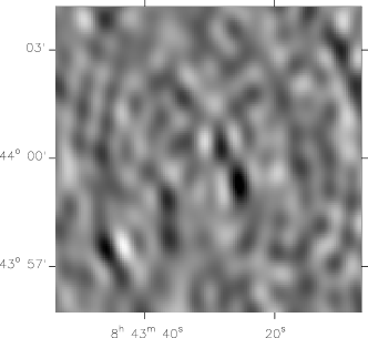
Figure 3: Long – i.e. greater than 1.5 k$\lambda$ – baseline map for the test data after the sources in Table 4 have been subtracted. The greyscale range is from -200 (light) to 200 $\mu$Jy beam^-1.

Table 4 shows the fluxes found. A comparison with the sources known to be in the model (Table 1) shows that the flux of source three is significantly different. There are two reasons for this. Firstly, not all the flux has been subtracted – see Figure 3. Secondly, the positions used have been determined from the unCleaned map, by searching for extrema with Maxfit. Occasionally, the relative positions of sources are such that one source is in the steepest part of a sidelobe of another, and Maxfit does not find an extremum that corresponds to that source. This has occurred in this case with source 4. In this situation, Maxfit is not used, and the position from the Clean method is used. The flux value from the unCleaned map in that position is then used. The reliance on the Clean method combined positional problems and with difficulties automating the process for large numbers of sources means that the “matrix method” has only been applied in simple cases with a few well separated sources.

Table 4: Source fluxes and positions from the matrix method.

Source number	Flux	Offset from pointing centre
	($\mu$Jy  beam-1)	(arcseconds)
1	2970	$-$9, 9.6
2	877	34, 15
3	8	$-$47, $-$42.8
4	142	$-$122, 99.9

2.4 The FLUXFITTER method

In an attempt to overcome the problems of the Clean and matrix methods, the FluxFitter algorithm was introduced. The algorithm that it uses is straightforward:

1. An initial model of the sky is made, using a set of parameters that represents the positions and fluxes of each source, including the SZ decrement. This model is determined from the long-baseline RT maps (either raw or Cleaned) and, for the SZ parameters, from the X-ray image.

2. The flux that the RT would observe is calculated for every visibility point.

3. The misfit between the model and real $uv$ data is then calculated as $\chi^{2}$.

4. The parameters are then varied to minimise $\chi^{2}$.

The best-fitting parameter values are then used to subtract the radio sources; this is done within Aips. There are two advantages to this method. It works almost entirely in the aperture plane; only the source identification and approximate position finding is done in the image plane. Working in the aperture plane is preferred because the noise distribution is known to be Gaussian. The second advantage of this method is in point (i): a simultaneous fit to the positions and fluxes of the point sources and the SZ decrement is a clear improvement over either of the previous methods as there is no arbitrary “long” and “short” baseline split, and it allows full use of all visibility data, which increases the signal-to-noise ratio for point-source measurements.

The initial parameters for the sources are still estimated by iterating the Clean method. In a complex situation with both bright and faint sources, the map is Cleaned, and then positions measured. These sources are then subtracted and the subtracted data then mapped again. This loop can be performed many times to estimate the number of sources and their approximate positions and fluxes. In a less complex situation, Clean is not used, and sources are approximately subtracted and then the data remapped. Again, this is just to provide an initial guess for FluxFitter.

Currently only the amplitude of the SZ decrement is varied. The other parameters that describe the decrement – position, core radius and $\beta$-parameter for the cluster – are all fixed in advance from the X-ray data. This is done as the radio data do not constrain well the core-radius or $\beta$ value; with present telescopes, the X-ray measurements constrain the core radius, $\beta$ value and position much better.

FluxFitter was run twice on the simulated test data. The fluxes and positions from the Clean method were used as an initial guess for the first run. The fluxes and positions from this run are shown in Table 5; the errors are those reported by FluxFitter – see below. After subtraction with Uvsub, the map of baselines greater than 1.5 k$\lambda$ was consistent with noise. For a second run, the fluxes and positions from the Clean method were used, and the positions of the additional two sources were also used. The fluxes and positions from this run are shown in Table 6. This table shows that the two additional sources are detected with good significance. That the overall noise level of 30 $\mu$Jy beam^-1 is lower than that for the Clean method is not surprising as all the baselines are being used in the determination of the fluxes and positions. After subtracting the six reported sources, a map of baselines shorter than 1.0 k$\lambda$ shows a decrement of flux $-700\pm 65$ mJy beam^-1 at an offset (9^′′,4^′′). FluxFitter itself finds a central decrement of $0.87\pm 0.08$ mK, close to the set value of 0.82 mK.

As an additional check, a third run of FluxFitter was performed, and the four sources found from the Clean method and two random points were used as the initial guess. In this case, FluxFitter reported that both of the two random “sources” had fluxes below the noise level and very large positional-errors.

Table 5: Source positions and fluxes as reported by FluxFitter using the Clean model as an initial guess. The formal error on each flux is 30 $\mu$Jy beam^-1.

Source number	Flux	Offset from pointing centre
	($\mu$Jy  beam-1)	(arcseconds)
1	3031	$-9.5\pm 0.1$, $9.6\pm 0.2$
2	966	$34.5\pm 0.3$, $15.3\pm 0.5$
3	208	$-47.5\pm 1.2$, $-42.8\pm 2.8$
4	184	$-122.3\pm 1.6$, $98.2\pm 2.8$

Table 6: Source positions and fluxes as reported by FluxFitter using additional information. The formal error on each flux is 30 $\mu$Jy beam^-1.

Source number	Flux	Offset from pointing centre
	($\mu$Jy  beam-1)	(arcseconds)
1	3024	$-9.9\pm 0.1$, $9.9\pm 0.2$
2	970	$34.9\pm 0.5$, $15.6\pm 0.7$
3	212	$-47.8\pm 1.8$, $-40.8\pm 3.6$
4	155	$-121\pm 2.6$, $98.8\pm 4.1$
5	140	$7.9\pm 3.8$, $-3.1\pm 4.2$
6	132	$67.4\pm 3.3$, $-64.8\pm 4.6$

FluxFitter also reports error bounds. As Figure 5 shows, the $\chi^{2}$ contours are elliptical and orientated along the variable axes, which shows that the parameters are independent. The error on each parameter is calculated by finding the parameter values at which the reduced $\chi^{2}$ increases by 1.

Figure 4: $\chi^{2}$ contours for the flux and position in Dec for the brightest source in the test field.The spacing between contour levels in each figure is such that the reduced $\chi^{2}$ value increases by 1 between each contour.

Figure 5: $\chi^{2}$ contours for position for the brightest source in the test field. The spacing between contour levels in each figure is such that the reduced $\chi^{2}$ value increases by 1 between each contour.

The error-bound reporting was checked by simulating a point source with differing signal-to-noise ratio. 500 observations of a single point source were simulated; the signal-to-noise was kept constant for groups of 10 simulations, and the position was held constant for all the simulations. The visibilities were simulated with Gaussian noise. The known position was then fed to FluxFitter as an initial guess, and the best-fitting position and flux recorded. It was found that the quoted error bar does enclose the position for 67% of the simulations. It was also found that the uncertainty of the position, that is the size of $\sigma$, varies as the inverse of the signal-to-noise. This result is shown in Figure 6. Note that this relation holds down to very low signal-to-noise ratios. The result is useful for determining whether a tentative source found with the RT at low signal-to-noise has a position coincident with higher significance data, for example from NVSS or POSS.

Figure 6: Signal-to-noise ratio verses the uncertainty (in arcseconds) of the position. Fitting a straight line to this data gives $\textrm{uncertainity}/\textrm{arcsec}=(13.7\pm 0.5)(\mathrm{signal/noise})^{-0.99\pm 0.01}$

2.4.1 Possible improvements

Source recognition is clearly the biggest problem that still remains. It is the only step that is still performed in the map plane rather than aperture plane. There are computational issues involved here: producing a map and identifying sources “by hand” is possible and fairly cheap in computer time, but the noise in the map plane is non-Gaussian. Minimising the misfit between the data and a given number of sources is also cheap; but allowing the number of sources to vary vastly increases the complexity of the problem and the time required. It is possible that more advanced minimising techniques such as simulated annealing (see e.g. Press et al. 1993) or using massive inference techniques will make this possible and robust in the aperture plane.

2.5 Comparison of results

Tables 3, 4 and 6 show the results of three different methods for source fitting. For both the Clean and FluxFitter methods, the results with six sources are considered. The positions and fluxes put into the model are shown in Table 1. The resultant position and depth of the SZ decrements after subtraction are shown in Table 7. The parameters are all measured from dirty maps, made with baselines shorter than 1 k$\lambda$. Note that the matrix method has a less deep SZ flux density, and that the FluxFitter and Clean method values are statistically consistent with the expected value for this model cluster ($-660$ $\mu$Jy beam^-1). Also, the positions of the SZ decrement are fully consistent with the model as the beam size is around 180^′′. It is not surprising that the flux of the SZ decrement from the matrix method is less deep as the central 100 $\mu$Jy source has not been subtracted. Also, the matrix method does an incomplete subtraction of the sources it does find, resulting in more contamination of the SZ signal. Note that this does not imply that the matrix method will always will give a lower SZ decrement if the source subtraction is incomplete.

Table 7: Parameters for the resulting SZ decrements from the simulated data.

Subtraction	SZ flux	position
method	($\mu$Jy  beam-1)	(arcseconds)
Clean	$-675\pm 72$	$-$4, $-$2
Matrix	$-500\pm 90$	18, 0
FluxFitter	$-700\pm 65$	9, 4

All three methods benefit from prior knowledge of the source distribution on the sky. This can be estimated from looking at lower frequency surveys such as NVSS or FIRST. Most falling-spectrum sources, i.e. with $\alpha>0$ (where $S\propto v^{-\alpha}$ where $v$ is the observing frequency and $\alpha$ is the spectral index) will be detected in NVSS and or FIRST. However, as shown by Cooray et al. [1998] in clusters and Taylor [2000] generally, there are rising spectrum sources, i.e. with $\alpha<0$ that are present at 15 GHz and not detected in NVSS and FIRST.

3 Observations of Abell 611

3.1 X-ray

Abell 611 is a cluster at $z=0.288$ [1995] originally identified by Abell [1957]. It has an 0.1–2.4 keV luminosity of $8.63\times 10^{44}$ W [], with a temperature of $7.95^{+0.56}_{-0.52}\times 10^{7}$ K [2000]. White derived this value from a 57-ks ASCA exposure by considering both a single-phase and two-phase cooling model. The temperature values found for the bulk of the gas are statistically equivalent and a mass deposit rate of $0^{+177}_{-0}$ $M_{\odot}$ yr^-1 was found for the cooling model.

The 17-ks ROSAT HRI observation from April 1996 is shown in Figure 7. The image contains two bright pixels, which, on comparison with the POSS image, are coincident with a large galaxy. These pixels were removed. We calculate an X-ray emissivity constant of 1.29$\times 10^{-69}$ counts s^-1 from 1 m³ of $7.95\times 10^{7}$-K gas of electron density 1 m^-3 at a luminosity distance of 1 Mpc, assuming a metallicity of $0.21\pm 0.07$ solar and an absorbing H column of $4.88\times 10^{24}$ m^-2.

The best-fitting model parameters were $\beta=0.59$, core radii of 26^′′ and 24^′′ with a position angle of the major axis of 101^∘ and a central electron density of $n_{0}=11.6\times 10^{3}$ m^-3 (assuming a core radius along the line of sight of $25=(24\times 26)^{1/2}$ arcsec and $H_{0}$= 50 km s^-1 Mpc^-1). There is a degeneracy between the core radii fitted and $\beta$ but this has no significant effect on $H_{0}$ (see Grainge et al. 2001b and Jones et al. 2001).

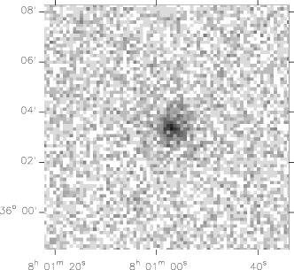
Figure 7: ROSAT HRI image of A611. The exposure time is 17 ks. The greyscale range is 0 to 32 counts.

3.2 RT observations

A611 was observed for 16 sets of 12 hours between November 1994 and January 1995 with the RT in configuration Cb. Flux and phase calibration and overall data reduction strategy are described in Grainge et al. [2001a]. Three days of data – taken in bad weather – were rejected after examining the 1-day maps and noise levels. A map of the combined 13 days of data using baselines longer than 1.5 k$\lambda$ had a noise level of 70 $\mu$Jy beam^-1, and only one source was visible, with flux 299 $\mu$Jy beam^-1 at $\rm{RA}\ 8^{h}\ 0^{m}\ 57^{s}1\$ $\rm{Dec.}\ +36^{\circ}\ 3^{\prime}\ 40^{\prime\prime}$. This source was removed with Uvsub, using the flux and position from the dirty map. A long-baseline map of the subtracted data was consistent with noise, with no other sources in the field.

Table 8 lists the sources found in the FIRST catalogue around the pointing centre for A611. The NVSS catalogue contains no sources in this region. Neither of the two FIRST sources is detected at 15 GHz and the source that is present at 15 GHz is not detected at lower frequencies.

Table 8: The radio sources in the FIRST catalogue within 400^′′ of the RT pointing centre for A611.

		Flux (mJy  beam-1)
RA	Dec	Peak
8 1 20.248	36 5 9.3	$1.25\pm 0.13$
8 0 54.948	36 9 6.1	$1.10\pm 0.13$

FluxFitter was then run using the X-ray data to provide a model of the SZ decrement and using all the baselines. Again, the initial guess was defined by the 1.5-k$\lambda$-only fitting. The source was found to be at $\rm{RA}\ 8^{h}\ 0^{m}\ 57^{s}1\$ $\pm 0.9$ $\rm{Dec.}\ +36^{\circ}\ 3^{\prime}\ 35^{\prime\prime}$0 $\pm 8$ with a flux of $188\pm 65$ $\mu$Jy  beam^-1, which is lower than the long-baseline only values. As the angular size of A611 is small, it is likely that the SZ signal was contaminating the “long”-baseline map. Note that this source is not detected in the FIRST survey, and so in this case prior knowledge from a lower frequency survey has not helped. Figure 8 shows a Cleaned map of baselines shorter than 1 k$\lambda$ after this source has been subtracted. The decrement (as measured from the map) is $-540\pm 125$ $\mu$Jy beam^-1 at $\rm{RA}\ 8^{h}\ 0^{m}\ 57^{s}3\$ $\rm{Dec.}\ +36^{\circ}\ 2^{\prime}\ 38^{\prime\prime}$. This location is 3^′′ in RA and 36^′′ in Dec away from the X-ray cluster location. Considering the Clean beam used is 92^′′$\times$ 350^′′, this is a good positional agreement between the X-ray and SZ observations. The slight extension to the south is not significant.

Figure 8: The SZ effect in A611. The contour levels are $-$480, $-$360, $-$240 and $-$120 $\mu$Jy beam^-1 (solid) and 120 $\mu$Jy beam^-1 (dashed). The map has been Cleaned; the restoring beam, which is 92^′′ by 350^′′ FWHM at a position angle 3.4^∘, is shown in the bottom left.

3.3 $H_{0}$ determination

From the source subtracted dataset and the X-ray parameters of the cluster, it is possible to estimate $H_{0}$, as described in Grainge et al. [2001b]. The likelihoods for different $H_{0}$ values are calculated and are shown in Figure 9. The best-fit $H_{0}$ for A611 is then $52^{+22}_{-14}$ km s^-1 Mpc^-1. The error quoted is due to the noise in the SZ measurement, and does not include any of the other sources of error in the determination. The additional sources of error are described fully in Grainge et al. [2001b]. For A611, the error from the SZ measurement is by far the most important, and the final $H_{0}$ value is $52^{+24}_{-16}$ km s^-1 Mpc^-1 for an Einstein-de-Sitter world model. Assuming a world model with $\Omega_{\Lambda}=0.7$, $\Omega_{\rm M}=0.3$, $H_{0}$=$59^{+27}_{-18}$ km s^-1 Mpc^-1 from this cluster.

Figure 9: Likelihood plot for different $H_{0}$ values from fitting to the source-subtracted SZ data from A611.

4 Conclusions

The problem of radio source contamination in interferometric SZ observations and methods to remove it have been investigated, demonstrating the following.

1. The non-linear Clean method can work well, but does not use all the available information and can over-complicate the problem.

2. The matrix method, though linear, fails in typical situations such as the one simulated here. The failure is mainly due to the high sidelobes from the Ryle Telescope; they make it difficult to determine accurate positions, and so fluxes, for sources close to each other on a map.

3. FluxFitter uses all the available information and produces the simplest model. It solves simultaneously for sources and SZ decrement, and it works with with the visibilities, where noise is known to be Gaussian, rather than in the map plane where the noise is correlated.

4. All three techniques suffer from the problem of source identification, which is currently performed in the image plane where the noise characteristics are complex. Source identification can be aided by prior information, for example from lower-frequency surveys.

5. The positional uncertainty, as determined in the aperture plane, is found to vary as $\textrm{uncertainity}/\textrm{arcsec}\propto(\mathrm{signal/noise})^{-0.99\pm 0.01}$ even at signal-to-noise ratios below nominal detection limits. The constant of proportionality will be a function of the interferometer used.

6. Observations of the cluster A611 with the Ryle Telescope give a 4.3-$\sigma$ detection of an SZ decrement, and combination with X-ray data gives and estimate of $H_{0}$= $52^{+24}_{-16}$ km s^-1 Mpc^-1, assuming an Einstein-de-Sitter cosmology, and $59^{+27}_{-18}$ km s^-1 Mpc^-1 using $\Omega_{\Lambda}=0.7$ and $\Omega_{\rm M}=0.3$.

5 Acknowledgements

We thank the staff of the Cavendish Astrophysics group who ensure the continued operation of the Ryle Telescope. Operation of the RT is funded by PPARC. WFG acknowledges support from a PPARC studentship. We have made use of the ROSAT Data Archive of the Max-Planck-Institut für extraterrestrische Physik (MPE) at Garching, Germany.

References

- [1957] Abell G. O., 1957, AJ, 62, 2
- [] Böhringer H., Voges W., Huchra J. P., McLean B., Giacconi R., Rosati P., Burg R., Mader J., Schuecker P., Simiç D., Komossa S., Reiprich T. H., Retzlaff J., Trümper, J., 2000, ApJS, 129, 435
- [1998] Cooray A. R., Grego L., Holzapfel W. L., Joy M., Carlstrom J. E., 1998, AJ, 115, 1388
- [1995] Crawford C. S., Edge A. C., Fabian A. C., Allen S. W., Bohringer H., Ebeling H., McMahon R. G., Voges W., 1995, MNRAS, 274, 75
- [1999] Das R., 1999, M.Phil. thesis, Cambridge University
- [1996] Grainge K., 1996, Ph.D. thesis, Cambridge University
- [1996] Grainge K., Jones M., Pooley G., Saunders R., Baker J., Haynes T., Edge A., 1996, MNRAS, 278, L17
- [2001a] Grainge K., Grainger W. F., Jones M. E., Kneissl R., Pooley G. G., Saunders R., 2001a, MNRAS, submitted
- [2001b] Grainge K., Jones M. E., Pooley G., Saunders R., Edge A., Grainger W. F., Kneissl R., 2001b, MNRAS, submitted
- [1994] Greisen E. (ed.), 1994, Aips Cookbook, NRAO
- [2001] Jones M. E., Grainge K., Grainger W. F., Pooley G., Saunders R., Edge A., Kneissl R., 2001, MNRAS, submitted
- [1972] King I. R., 1972, ApJ, 174, L123
- [1989] Perley R. A., Schwab F. R., Bridle A. H. (ed.), 1989, ASP Conf. Ser. 6: Synthesis Imaging in Radio Astronomy
- [1993] Press W. H., Teukolsky S. A., Vetterling W. T., Flannery B. P., Lloyd C., Rees P., 1993, Numerical Recipes in FORTRAN - the Art of Scientific Computing, 2nd edn. Cambridge University Press
- [2000] Reese E. D., Mohr J. J., Carlstrom J. E., Joy M., Grego L., Holder G. P., Holzapfel W. L., Hughes J. P., Patel S. K., Donahue M., 2000, ApJ, 533, 38
- [1970] Sunyaev R., Zel’dovich Y., 1970, Comments Astrophys. Space Phys., 2, 66
- [1972] Sunyaev R., Zel’dovich Y., 1972, Comments Astrophys. Space Phys., 4, 173
- [2000] Taylor A., 2000, IAU Symposium. 201, 5
- [2000] White D. A., 2000, MNRAS, 312, 663