The Clustering of Hot and Cold IRAS Galaxies: The Redshift Space Correlation Function

Abstract

We measure the autocorrelation function, $\xi$, of galaxies in the IRAS Point Source Catalogue galaxy redshift (PSCz) survey and investigate its dependence on the far-infrared colour and absolute luminosity of the galaxies. We find that the PSCz survey correlation function can be modelled out to a scale of $10\;h^{-1}{\rm Mpc}$ as a power law of slope $1.30\pm 0.04$ and correlation length $4.77\pm 0.20$. At a scale of $75\;h^{-1}{\rm Mpc}$ we find the value of $J_{3}$ to be $1500\pm 400$.

We also find that galaxies with higher $100\mu m/60\mu m$ flux ratio, corresponding to cooler dust temperatures, are more strongly clustered than warmer galaxies. Splitting the survey into three colour subsamples, we find that, between 1 and $10\;h^{-1}{\rm Mpc}$, the ratio of $\xi$ is factor of 1.5 higher for the cooler galaxies compared to the hotter galaxies. This is consistent with the suggestion that hotter galaxies have higher star-formation rates, and correspond to later-type galaxies which are less clustered than earlier types.

Using volume limited sub-samples, we find a weak variation of $\xi$ as a function of absolute luminosity, in the sense that more luminous galaxies are less clustered than fainter galaxies. The trend is consistent with the colour dependence of $\xi$ and the observed colour-luminosity correlation, but the large uncertainties mean that it has a low statistical significance.

1 Introduction

The relation between the distribution of galaxies and the distribution of mass is now one of the most important problems in large-scale structure. Empirically, it has been found that different galaxy types have different clustering amplitudes and hence that galaxies are biased tracers of the mass distribution. Evidently, we need to understand the physical mechanisms responsible for these biases if we are to establish the connection between galaxy tracers and the mass. This problem can be understood in terms of two related questions: (i) How does the clustering of a galaxy sample depend on the properties of the galaxies? and (ii) How do the properties of galaxies depend on their local environment?

Many ideas have been put forward as to how the environment may modify galaxy properties, from schematic ideas concerning feedback in the formation process (White & Rees 1978; Dekel & Rees 1987) to hydrodynamical simulations of galaxy formation incorporating cooling and dissipation (e.g. Katz & Gunn 1991; Navarro & White 1993; Pearce et al. 1999). Over the next few years we can expect major advances in hydrodynamic simulations employing parallel computers and there is a real prospect of understanding the relationship between galaxy morphologies and environment within the context of specific theories of cosmological fluctuations. We can hope that such numerical simulations will eventually be able to provide detailed predictions of the spatial distribution of galaxies as a function of their stellar content, rotation velocity, star-formation rate, and morphological type.

The simplest bias schemes are those based on the statistics of high density peaks (Kaiser 1984, Mo & White 1996). Since the optical magnitude of a galaxy is correlated to the depth of the potential via the Tully Fisher relation for spirals and $D_{n}-\sigma$ relation for ellipticals, this would suggest that the brightest galaxies will be more strongly correlated than fainter galaxies. Realistic galaxy formation models rely on feedback mechanisms to limit star-formation, either acting internally within each galaxy or involving interactions with other galaxies and the intergalactic medium. So galaxies in regions of high local galaxy density are likely to have a reduced star-formation rate (SFR). Indeed this is confirmed by the observation that later-type optical galaxies, which have higher SFRs, have a much lower clustering amplitude than earlier galaxy types (e.g. Rosenberg, Salzer & Moody 1994; Loveday et al. 1995; Loveday, Tresse & Maddox 1999).

Galaxies with a high SFR tend to be bright in the far infra-red (FIR) because of the thermal emission from dust heated by young stars. Thus the observations that IRAS galaxies (selected on their $60\mu$m flux) tend to avoid rich galaxy clusters, and have a lower clustering amplitude are consistent with this general picture. In this paper we divide the PSCz sample of IRAS galaxies into subsamples based on their FIR colour. Since the galaxies with warmer FIR colours are those with higher SFR, we can further test the dependence on star-formation rate. Mann, Saunders & Taylor (1996) selected warm and cool sub-samples of IRAS galaxies from the QDOT survey based on their 60$\mu m$/100$\mu m$ flux ratio, and found marginal evidence that warmer galaxies are more strongly clustered than cooler galaxies, the opposite to what is expected from the morphology density relation. However they did not consider the result very significant compared to the expected cosmic variance.

Using optical galaxy samples, a number of authors have found indications of changes of the clustering amplitude with galaxy luminosity, (e.g. Valls-Gabaud, Alimi & Blanchard 1989; Park et al. 1994; Moore et al. 1994; Loveday et al. 1995; Benoist et al. 1996) but the samples are small and the observed amplitude shifts do not have a high statistical significance. The expected luminosity dependence for IRAS galaxy samples is less clear, since the FIR luminosity of a galaxy is likely to depend on both the mass of its dark halo and its specific SFR. If the FIR luminosity is correlated to the halo mass, then brighter galaxies should have a higher clustering amplitude. On the other hand, a high SFR will make a galaxy more luminous, and galaxies with a high star-formation rate tend to have weaker clustering. It is not easy to predict which of these is the dominant effect. Observationally Szapudi et al. (2000) and Beisbart & Kerscher (2000) have used mark correlation functions with volume limited sub-samples to examine the luminosity dependence of clustering in the PSCz survey. Over the narrow range of luminosities they consider they concluded that there is no significant luminosity dependence.

In this paper we investigate clustering amplitude for different sub-samples of galaxies from the PSCz survey. We begin by summarizing the relevant aspects of the PSCz survey and describe various sub-samples that we will study here. In Section 3 we show our methods and in Section 4 we give our results for the whole sample and consider how the amplitude of the redshift space autocorrelation function depends on the colour and luminosity selection of the galaxies. Finally, we discuss our conclusions in Section 5.

2 The PSC Redshift survey

2.1 Description

Galaxies for the PSCz were selected from the IRAS Point Source Catalogue (Beichman et al. 1988) by positional, identificational flux and colour criteria designed to accept almost all galaxies while keeping contamination by Galactic sources to an acceptable level. The significant differences compared with the QDOT survey (Lawrence et al. 1999), were that the colour criteria were relaxed to avoid excluding previously uncatalogued galaxies with unusual (especially cool) colours and the sky coverage is increased to 84 per cent by including areas of high cirrus contamination. These changes increase the contamination of the galaxy catalogue from local galactic sources (stars, planetary nebulae, cirrus etc) but ensure the sample has a higher completeness. The contaminating Galactic sources were excluded by a combination of IRAS and optical properties (from sky survey plates), and where necessary spectroscopy. Redshifts were taken from all available published or unpublished sources; principally Huchra’s ZCAT, the LEDA database, the 1.2Jy and QDOT surveys. Also 4500 new redshifts were taken on the Isaac Newton Telescope, the Anglo-Australian Telescope, the Cerro-Tololo 1.5-m and Cananea 2.1-m telescopes. In total the catalogue contains 14677 redshifts and the median redshift is $\sim 0.028$. The uniformity and completeness of the catalogue are discussed by Saunders et al. (2000).

The redshift distribution of the galaxies is shown in Figure 1. It can be seen that the peak of the distribution is near $z=0.02$, and there is a tail which extends out to beyond $z=0.1$. This tail means that there are over 1200 galaxies in the survey with a redshift $>$ 0.08.

For our present analysis, only galaxies with a redshift $>$ 0.004, corresponding to a recession velocity of 1200 ${\rm km\;s}^{-1}$ were selected, so that local effects and the velocity uncertainties of around 120 ${\rm km\;s}^{-1}$ were less significant.

(a)

(b)

Figure 1: The redshift distributions for galaxy samples. (a) colour selected sub-samples listed in Table 1. (b) absolute luminosity selected sub-samples listed in Table 2.

2.2 Sub-samples

2.2.1 Colour sub-samples

In order to investigate the dependence of clustering on the temperature of the galaxies, we used the addscan $60\mu m$ and $100\mu m$ fluxes ($f_{60}$ and $f_{100}$) to sub-divide the parent redshift catalogue into three sub-samples: hot galaxies, with $f_{100}/f_{60}<1.7$ ; warm galaxies, with $1.7<f_{100}/f_{60}<2.3$; and cold galaxies, with $f_{100}/f_{60}>2.3$. These boundaries correspond to blackbody temperatures of around 31 and 28K, and were chosen to give roughly equal numbers in each sub-sample. The actual numbers of galaxies in the sub-samples were 4452, 4388 and 4107 respectively. The mean $f_{100}/f_{60}$ colour ratios for the hot, warm and cold sub-samples were 1.31, 1.98 and 2.91 respectively, corresponding to black-body temperatures of about 34K, 30K and 26.5K respectively. The mean for the whole catalogue is 2.05, corresponding to a black-body temperature of around 29.5K.

The redshift distributions for the sub-samples are plotted in Figure 1(a) and it can be seen that the cooler samples tend to peak at a slightly lower redshift than the hotter samples. This reflects the correlation between colour and absolute luminosity as plotted in Figure 2: cooler galaxies tend to be fainter, and so are only seen nearby. Nevertheless, these differences in redshift distributions are smaller than the difference for luminosity selected sub-samples, as discussed in the next section.

The angular distribution of these sub-samples are plotted in Figure 3. It can be seen that these samples show no obvious gradients as a function of position on the sky, and also that the cooler sample appears to be more strongly clustered. Figure 4 shows the projection of the galaxies on to a plane along the celestial equator. Again the cooler sample appears more clustered than the warmer samples. Though apparently quite significant, these visual impressions should be treated with caution. The cooler sample is shallower than the warmer samples, so the angular clustering would be stronger, even if the samples had the same spatial clustering. Also the cool sample has a higher space density than the warmer samples, and this may enhance the visual appearance of clustering.

Figure 2: Log plot of absolute luminosity at 60$\mu m$ against the $100\mu m/60\mu m$ colour. The vertical lines show the boundaries used to select our colour sub-samples, and the horizontal line shows the boundary between the luminosity samples.

(a)

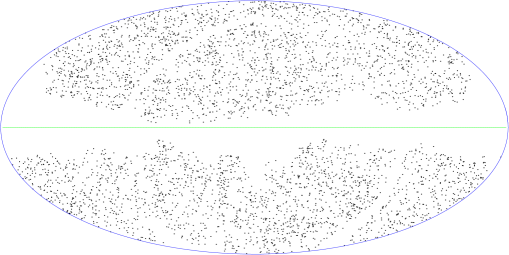
(b)

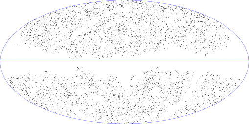
(c)

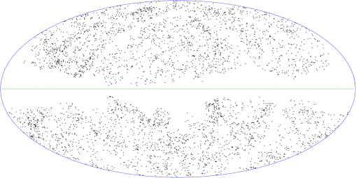
Figure 3: Plots of the position of galaxies on the sky for the three colour sub-samples listed in Table 1: (a) hot, (b) warm, and (c) cold. The line shows the Galactic equator and the obscuration around this is masked out in the analysis.

(a) (b)

(c) (d)

Figure 4: The galaxy positions projected onto the celestial equator for the full survey and the three colour sub-samples listed in Table 1: (a) all, (b) hot, (c) warm, and (d) cold.

2.2.2 Absolute luminosity sub-samples

The parent sample was also divided into sub-samples of absolute luminosity at $60\mu m$: faint galaxies, with $\log_{10}(L_{60})<9.6$; and bright galaxies with $\log_{10}(L_{60})>9.6$, where $L_{60}=4\pi d^{2}f_{60}$ and $d$ is the luminosity distance to the galaxy (we assumed $\Omega=1$ and $\Lambda=0$ to determine the geometry, but at the distances considered here, cosmological effects are negligible.) The units of $L_{60}$ are $L_{\odot}h^{-2}.$ Note that the usual definition of an ultra-luminous IRAS galaxy corresponds to $\log_{10}(L_{60})\mathrel{\hbox to0.0pt{\lower 3.0pt\hbox{$\mathchar 536\relax$}\hss}\raise 2.0pt\hbox{$\mathchar 318\relax$}}11.4$ (Soifer et al 1987), and so the lower limit of our brighter sample is a factor of $\sim$ 60 fainter than ultra-luminous galaxy samples.

The bright sample has a higher mean redshift, and hence covers a much larger volume, but the galaxies are a more dilute sampling of the density field and so a larger number is needed to give a similar number of small separation pairs. Hence the faint and bright samples were chosen to have 4719 and 8228 galaxies respectively.

The redshift distribution for these sub-samples is shown in Figure 1(b). Since the parent sample is flux limited, the low luminosity galaxies have a sharply defined upper redshift limit corresponding to the distance where the observed flux equals the flux limit. For the more luminous galaxies, the clustering signal is dominated by the volume at higher redshifts. This means that the clustering measurements for the two samples come from almost independent volumes, and so cosmic variance introduces a large uncertainty in the comparison. The clustering measurements for colour selected sub-samples are less affected by cosmic variance because they cover very similar volumes, and so their comparison should be more reliable.

2.2.3 Volume limited sub-samples

The cosmic variance between the luminosity sub-samples can be partly overcome by using volume limited sub-samples. To do this, the parent catalogue was split into sub-samples limited by distance and also by absolute luminosity. Galaxies within a sphere of radius $x$, centred on us, are included only if their absolute luminosity ($L_{60}$) is greater than $4\pi x^{2}f_{min}$, where $f_{min}$ is the flux-limit of the survey or sample (0.6 Jy for the full PSCz survey). Without galaxy evolution these samples will be homogeneous. Unfortunately the numbers of galaxies in these samples, shown in Table 3, are rather small.

IRAS galaxies are known to show very rapid evolution (Saunders et al 1990), and this could introduce a radial gradient in space density in the volume-limited samples. Figure 5 shows the galaxy number density as a function of radius, normalised so that the maximum radius of the volume is 1, for the samples with radius 100, 150, 200 and 300$\;h^{-1}{\rm Mpc}$. No significant gradients are apparent, and so we assume a constant density in our clustering estimates. These sub-samples allow another test for a luminosity trend in the clustering as the larger volumes are limited to brighter galaxies than the smaller volumes. Note that the different volumes have a significant fraction of galaxies in common, so that the results for different volume scales are not completely independent.

2.3 PSCz mock catalogues

Large N-body simulations from Cole et al. (1998) were used to create mock PSCz surveys. The simulations used the $AP^{3}M$ code of Couchman (1991) loaded with $192^{3}$ particles of mass $1.64\times 10^{12}\Omega_{0}h^{-1}M_{\odot}$ in a box with a co-moving size of $345.6h^{-1}{\rm Mpc}$. More details can be found in Cole et al. (1998). For this analysis three different cosmological models have been considered. They are a spatially flat low density universe model ($\Lambda CDM$) with $\Omega_{0}=0.3$, $\Omega_{\Lambda}=0.7$ and $\Gamma=0.25$, a spatially flat universe model ($SCDM\Gamma_{0.25}$) with $\Omega_{0}=1.0$ and $\Gamma=0.25$, and finally a spatially flat universe model ($SCDM_{cobe}$) with $\Omega_{0}=1.0$ and $\Gamma=0.5$, normalised to match the amplitude of the COBE data. For pure CDM-type models the shape parameter, $\Gamma=\Omega h$.

The galaxy catalogues were extracted from the numerical simulations by first identifying a population of objects with similar properties to the Local Group (LG). Then an observer is placed by considering the observational constraints of peculiar velocity, local overdensity and shear. All points within a sphere of $120h^{-1}{\rm Mpc}$ radius around the observer are included, and the frame is rotated so that the motion of the observer is the same as the LG peculiar velocity. Note that this sphere radius is less than the size of the PSCz survey. A luminosity was randomly assigned to each galaxy in the mock realizations to mimic the corresponding observational properties. The PSCz density is reproduced by using the PSCz selection function to reject points and also to randomly assign a flux to each point. Unsurveyed regions are rejected using the PSCz mask to give the same sky coverage as the real catalogue. Each mass point is associated with a galaxy so the linear bias parameter, $b=1.0$. Lastly the bias against early-type galaxies in the original IRAS survey is introduced by rejecting an appropriate fraction of galaxies in clusters the cores of clusters, which is meant to reproduce Dressler’s morphology-density relation (Dressler 1980). The resulting mock surveys have approximately the same correlation function, redshift distribution and flux distribution as the real PSCz sample.

We calculated the correlation function for the 10 realizations of each model, and used the standard deviation about the mean of $s_{0}$ and $\gamma$ to estimate of the uncertainties in these measurements for the real sample. These catalogues can also be split into the same bright and faint sub-samples as the real catalogue. Again, the standard deviation between the realizations gives an estimate of the uncertainty on the measurements for the real data, and so allows more reliable estimates of the significance level of any variations seen in the real data. Colours can be included in the mocks by considering Figure 2, which we modelled as a linear relation between $\log_{10}(f_{100}/f_{60})$ and $\log_{10}(L_{60})$ with a Gaussian dispersion about the mean. Each galaxy can then be assigned a colour according to its luminosity, $\log_{10}(f_{100}/f_{60})=A\log_{10}(L_{60})+B+C$, where $A=-0.117$, $B=1.427$ and $C$ is a random number selected from a Gaussian distribution with variance of 0.2. Then colour sub-samples can be selected and tested in the same way as the real data. Since the luminosities were assigned at random to the mock galaxies, and the colours are based on the luminosities, the clustering in the mocks is independent of luminosity and colour.

3 Methods for estimating the redshift space autocorrelation function $\xi$

There has been considerable interest in analysing the best way to estimate the autocorrelation function from redshift surveys (e.g. Landy & Szalay 1993; Vogeley & Szalay 1996; Hamilton 1997a,b). Reliable and unbiased estimates can be obtained by cross-correlating the real data with an artificial unclustered catalogue which has the same selection functions in angle on the sky and in redshift. We create this catalogue by generating random positions uniformly over the sky, and rejecting positions behind the mask which defines the boundaries of the real data. For each position we then assign a redshift from a distribution which matches the observed data.

We investigated several methods to generate the redshift distribution for the random catalogues: random shuffling of the positions on the sky relative to the redshifts; random shuffling followed by adding a further random velocity from a Gaussian distribution with $\sigma=500,1000$ or $1500~{}{\rm km\;s}^{-1}$; and generating a random redshift distribution to match an analytic fit to the selection function (Saunders et al. 2000). For the full catalogue we found that random shuffling with $1000~{}{\rm km\;s}^{-1}$ smoothing and the analytic fit gave indistinguishable results for $\xi$. Rather than calculating a best fit selection function for each sub-sample we simply generated appropriate sub-samples using the $1000~{}{\rm km\;s}^{-1}$ smoothed randomized distribution. For each random catalogue we generated 12 times the number of random points as real galaxies for the whole sample, and 20 times as many for the sub-samples.

3.1 Flux limited sample methods

The estimate of $\xi(s)$ we used (Landy & Szalay 1993) is given by

$$\xi(s)={\langle DD\rangle-2\langle DR\rangle+\langle RR\rangle\over\langle RR\rangle},$$ (1)

where $\langle DD\rangle$ is the weighted sum over galaxy pairs with separation $s$ in redshift space; $\langle RR\rangle$ is the weighted sum of pairs with the same separation in the random catalogue; and $\langle DR\rangle$ is the weighted sum of galaxy-random pairs. In each of these sums, the pairs at separation $s$ are weighted by a factor

$$w_{ij}=\frac{1}{(1+4\pi n(z_{i})J_{3}(s))(1+4\pi n(z_{j})J_{3}(s))},$$ (2)

where $n(z_{i})$ is the space density of observed galaxies at the redshift $z_{i}$ for galaxy $i$, and $J_{3}(s)=\int_{0}^{s}\xi(r)r^{2}dr$ (Efstathiou 1988).

To calculate $\xi(s)$ we first calculated $\xi(s)$ with a standard pair weighting of the sample and fitted a power law to the results for $1<s<10~{}h^{-1}{\rm Mpc}$. We then recalculated the correlation function using $J_{3}$ from this best fit power law, truncated so that the maximum $J_{3}$ is 1500. It was found that only one iteration was needed to produce a stable result with a consistent $J_{3}$ and $\xi$. The calculation of $\xi(s)$ is relatively insensitive to the precise form of the $J_{3}$ weighting employed. We then fit the final correlation function with a power law of the form:

$$\xi(s)=\left(\frac{s}{s_{0}}\right)^{-\gamma}.$$ (3)

We calculate the correlation function for mock catalogues in the same way as for the real sample.

3.2 Volume limited sub-sample methods

For the volume-limited sub-samples a different technique was used to estimate the correlation functions. Following the method of Croft et al. (1997), we used a maximum likelihood approach that assumes that each distinct galaxy pair is an independent object. This technique uses the fact that $1+\xi(s)$ can be considered as the probability distribution for galaxy pairs as a function of separation. Thus a power law $\xi$ can be fitted directly to the galaxy pair distribution without the need to specify arbitrary bins of pair separation. The resulting power law parameters tend to be more robust than fitting to a binned version of $\xi$, especially for small samples. The homogeneity of volume limited samples means that simple unit pair weighting yields the best results.

If galaxy pairs were independent, the calculated likelihood contours would directly provide 1-$\sigma$ uncertainties in the best-fit parameters, equivalent to the Poisson error in the pair counts. Since galaxy pairs are correlated, the effective number of pairs is reduced, and so the uncertainties are increased by a factor $(1+4\pi nJ_{3})$. These corrected Poisson estimates still do not allow for any uncertainty introduced by the variance in mean density on the scale of sample size. We used a simple approach to include this effect, by considering the variance in the mean density within the sample volume, ${\rm var}(\delta n/n)=3J_{3}/R^{3}$, where $R$ is the radius of the volume. This introduces an uncertainty in $\xi$, which we add in quadrature to the corrected Poisson estimates.

For volumes with radius $R\leq 100\;h^{-1}{\rm Mpc}$ we have also analysed the ten $\Lambda CDM$ mock catalogues using the same method. The $\Lambda CDM$ model was chosen because its clustering amplitude is the closest match to the observed amplitude. The standard deviation between results provides an independent estimate of the uncertainties in $s_{0}$ for each sample. For the volumes we consider (with radius $R\geq 50\;h^{-1}{\rm Mpc}$) the value of $J_{3}$ is roughly constant, and we find that the two methods agree to $\sim$10% if we choose $J_{3}=1500$. For volumes with radius $R>100\;h^{-1}{\rm Mpc}$ the mock catalogues are too small, and so we have to rely on the analytical approximation to estimate the uncertainties.

4 Results

4.1 Full sample

Our estimate of $\xi(s)$ for the full sample is shown in Figure 6. The power law fit gives $s_{0}=4.77\pm 0.20$ and $\gamma=1.30\pm 0.04$. The errors are estimated from the standard deviation between the ten realizations of the $\Lambda CDM$ mock catalogues. We calculated the value of $J_{3}$ and found it to be $1500\pm 400$ at a scale of $75\;h^{-1}{\rm Mpc}$. The error on the $J_{3}$ result is from the standard deviation of the mock realization results.

4.2 Colour sub-samples

Our estimates of the redshift-space correlation functions for the three colour sub-samples are shown in Figure 7. The error bar for each point shows the standard deviation between 10 realizations of the $\Lambda CDM$ mock catalogues. It is clear that over the range $1<s<10~{}h^{-1}{\rm Mpc}$ the amplitude of $\xi$(s) is higher by about a factor of 1.5 for the cooler sub-sample. Fitting a power law to the data over the range of $1<s<10~{}h^{-1}{\rm Mpc}$ gives parameters as shown in Table 1, clearly confirming the increase in clustering amplitude for cooler galaxies. Figure 8 shows $\chi^{2}$ contours for the hot and cold sub-sample, and suggests that trend is significant at about the $2\sigma$ level.

Since the best-fit $s_{0}$ and $\gamma$ are correlated, we have also fitted the data using a fixed value for $\gamma$, set to the best fit value for the full sample, $\gamma=1.30$. The resulting $s_{0}$ values for the three different colour sub-samples are listed in Table 1 and plotted as a function of mean colour in Figure 9. The trend of increasing $s_{0}$ for warmer galaxies is clearly apparent at about the $3\sigma$ level. A simple linear regression to the points yields

$$\log_{10}(s_{0})=0.24\log_{10}(\frac{f_{100}}{f_{60}})+0.61.$$ (4)

Analyzing colour selected sub-samples from the mock catalogues shows no significant difference in amplitude between the hot and cold sub-samples. This is as expected since we assigned the colours at random, but the measurements provide an important check that there are no subtle biases in our algorithms.

Figure 5: Galaxy number density plotted against normalised radius for the volume limited samples with radii labelled.

Table 1: Power law fit parameters to the colour sub-samples

Free parameter best fits:
colour range	$s_{0}$	$\gamma$
$f_{100}/f_{60}<1.7$	4.41 $\pm$ 0.29	1.32 $\pm$ 0.06
$1.7<f_{100}/f_{60}<2.3$	4.76 $\pm$ 0.30	1.21 $\pm$ 0.06
$f_{100}/f_{60}>2.3$	5.49 $\pm$ 0.29	1.25 $\pm$ 0.05
Fixed $\gamma$ at 1.30:
colour range	$s_{0}$
$f_{100}/f_{60}<1.7$	4.43 $\pm$ 0.30
$1.7<f_{100}/f_{60}<2.3$	4.64 $\pm$ 0.33
$f_{100}/f_{60}>2.3$	5.38 $\pm$ 0.30

Table 2: Power law fit parameters to the luminosity sub-samples

Free parameter best fits:
luminosity range	$s_{0}$	$\gamma$
$log(L_{60})<9.6$	4.96 $\pm$ 0.44	1.21 $\pm$ 0.04
$log(L_{60})>9.6$	4.80 $\pm$ 0.31	1.36 $\pm$ 0.06
Fixed $\gamma$ at 1.30:
luminosity range	$s_{0}$
$log(L_{60})<9.6$	4.82 $\pm$ 0.54
$log(L_{60})>9.6$	4.89 $\pm$ 0.35

Figure 6: Logarithmic plot of $\xi$ against $s$ for the full PSCz sample. The dotted line is the best-fit power-law, fitted for $1<s<10\;h^{-1}{\rm Mpc}$. The inset shows a linear plot of $\xi$ against $s$. The error bars are derived from the scatter between ten realizations of the $\Lambda CDM$ mock galaxy catalogues.

Figure 7: Logarithmic plots of $\xi$ against $s$ for the colour sub-samples defined in Table 1. The inset shows a linear plot of $\xi$ against $s$. The error bars are derived from the scatter between ten realizations of the $\Lambda CDM$ mock galaxy catalogues. For clarity, error bars are plotted only for the warm sub-sample.

4.3 Luminosity sub-samples

The estimates for the two luminosity sub-samples are shown in Figure 10. The error bars are derived from the scatter between ten realizations of the $\Lambda CDM$ mock galaxy catalogues. It is clear that there is very little difference between the two sub-samples. The power law fit parameters are shown in Table 2. These parameters show no significant difference when the errors are taken into account.

For all mock catalogues we found no difference between the results for the faint and bright sub-samples within the errors. This is as expected since we assigned the luminosities at random, but the measurements provide an important check that there are no subtle biases in our algorithms.

4.4 Volume limited sub-samples

Our results from the volume limited sub-samples are shown in Table 3 and displayed in Figure 11. Although there is clearly a hint of a trend of reducing amplitude with scale, it can be seen that the error bars are too large to say that this is a statistically significant relation.

The minimum absolute luminosity in the volume limited samples increases with the radius of the volume, so the mean luminosity also increases. Figure 12 explicitly shows the clustering amplitude as a function of the mean luminosity in the volume limited samples.

Table 3: Maximum likelihood fits to the volume limited sub-samples with $\gamma$ fixed at 1.30, and uncertainties estimated as described in Section 3.2.

Volume radius	no. of	$\left\langle\log_{10}\left(\frac{L_{\phantom{\odot}}}{L_{\odot}}\right)\right\rangle$	$s_{0}$
($h^{-1}{\rm Mpc}$)	galaxies		($h^{-1}{\rm Mpc}$)
50	1699	9.41	5.11 $\pm 1.19$
75	2151	9.71	4.91 $\pm 0.65$
100	2188	9.94	4.23 $\pm 0.44$
125	1961	10.12	4.90 $\pm 0.38$
150	1633	10.28	5.25 $\pm 0.42$
175	1399	10.41	3.86 $\pm 0.53$
200	1202	10.53	3.56 $\pm 0.74$
225	958	10.64	2.83 $\pm 1.08$
250	779	10.74	4.35 $\pm 1.43$
275	653	10.83	4.49 $\pm 2.00$
300	587	10.91	3.65 $\pm 2.50$

Figure 8: Contours of $\chi^{2}$ as a function of $s_{0}$ and $\gamma$ for the power-law fits to $\xi$ of the hot and cold sub-samples as in Table 1.

Figure 9: Clustering length $s_{0}$ versus mean colour for $\gamma$ = 1.30. The filled points show the colour sub-samples as defined in Table 1, and the open point shows the full catalogue. The best fit line is also shown and has the form $\log_{10}(s_{0})=0.24\log_{10}(\frac{f_{100}}{f_{60}})+0.61$.

Figure 10: Logarithmic plots of $\xi$ against $s$ for the luminosity sub-samples defined in Table 2. The inset shows a linear plot of $\xi$ against $s$. The error bars are derived from the scatter between ten realizations of the $\Lambda CDM$ mock galaxy catalogues. For clarity, error bars are plotted only for the bright sub-sample.

Figure 11: Clustering length $s_{0}$ versus volume radius for the volume limited sub-samples for a fixed $\gamma$ = 1.30. The error bars show the overall uncertainties including both Poisson errors in the pair counts, and an estimate of the cosmic variance as described in Section 3.2. For volumes with radius $R<100\;h^{-1}{\rm Mpc}$ we also estimated the uncertainties from the standard deviation between the ten realizations of the $\Lambda CDM$ mock catalogues and found good agreement with the analytic estimates.

5 Conclusions and discussion

We detect a colour dependence in the clustering of PSCz galaxies: the cooler galaxies are more strongly clustered than the hotter galaxies. Although the significance level of amplitude variations is not high, this does not mean that the effects are small: the clustering amplitude differs by a factor of 1.5 between the warm and cool sub-samples. We do not detect any significant variation in clustering for luminosity selected subsamples. Volume limited sub-samples show a slight trend corresponding to a weaker clustering for brighter galaxies, but the uncertainties mean it is not significant.

Our results are different to those of Mann, Saunders & Taylor (1996) who found marginal evidence that warmer galaxies are more strongly clustered than cooler galaxies. The main reason for the difference is simply the factor of 6 increase in number of galaxies in our sample, which dramatically reduces the uncertainties in our clustering estimates. The uncertainties on the earlier measurements encompass our results, so there is actually no discrepancy.

The variation of clustering with FIR colour that we find in the PSCz is consistent with the variation with star-formation rate indicated by H$\alpha$ and O[II] emission lines in the SAPM survey (Loveday et al. 1999). Loveday et al. split the SAPM survey into three samples with low, medium and high H$\alpha$ equivalent widths (EW), and estimate $s_{0}$ for the samples to be 8.7, 5.5 and 4.6 $h^{-1}{\rm Mpc}$ respectively. A similar split into low, medium and high O[II] EW samples gives $s_{0}$ values of 8.6, 4.9 and 4.1 $h^{-1}{\rm Mpc}$ respectively. The low EW samples are early type galaxies, which do not appear in IRAS samples. The medium and high EW samples are actively star-forming galaxies, which are more similar to IRAS samples. The clustering amplitude of the medium and high EW galaxies is very similar to that of the IRAS galaxies, suggesting that they do indeed trace a similar population. Furthermore, the change in $s_{0}$ between the medium and high SAPM emission-line galaxies is very similar to the change between cold and hot PSCz galaxies as seen in Figure 9.

The luminosity dependence is a more complex effect, because the FIR luminosity of a galaxy depends on both the mass of dust, and the recent star-formation rate. If the dust mass is correlated with the halo mass, then more luminous galaxies will, on average, be in more massive halos, which are expected to have a higher clustering amplitude. On the other hand, a high star-formation rate will make a galaxy more luminous, and galaxies with a high star-formation rate tend to be less clustered. It is not obvious which will be the dominant effect.

Given the correlation between colour and luminosity seen in Figure 2 we can infer the luminosity dependence from the colour dependence seen in Figure 9. From Figure 2 we find $\log_{10}(\frac{f_{100}}{f_{60}})=-0.117\log_{10}(L_{60})+1.427$, and so together with equation 4 we would expect $\log_{10}(s_{0})=-0.028\log_{10}(L_{60})+0.95$. This relation is plotted as the dashed line on Figure 12, and it can be seen that it is consistent with the data points. The luminosity variation seen in optical galaxy samples is approximately of the form $\log_{10}(s_{0})=4.37(0.7+0.3\frac{L}{L^{*}})$ (Benoist et al. 1996). The dotted line shows this with $L^{*}=3.6\times 10^{9}L_{\odot}$ (Springel & White 1998). This is clearly inconsistent with the trend seen in the PSCz sample.

The small decrease in clustering that we find for more luminous galaxies is consistent with the colour dependence effect alone, with no evidence for an increase in clustering for more luminous galaxies. If the standard picture of high-peak biasing is correct, we conclude that there is a very weak correlation between the FIR luminosity of a galaxy and the mass of it’s dark-matter halo. However, models which allow a variable number of galaxies per dark halo, and include scatter about the mean mass-luminosity relation lead to a very weak luminosity dependence of clustering (Somerville et al. 1999).

Finally we note that our present analysis has been restricted to the redshift space correlation functions. This means that any differences in the velocity distributions of the different sub-samples of galaxies will affect the amplitude of $\xi(s)$, particularly on small scales where the velocity separations are comparable to the random peculiar velocities. We consider these effects in a future paper.

Figure 12: Log plot of clustering length $s_{0}$ versus mean absolute luminosity for the volume limited sub-samples (filled circles), the bright and faint sub-samples (open circles) and the whole sample (open square). The dashed line shows the trend expected from the colour dependence seen in Figure 9 and the luminosity-colour correlation in Figure 2. The dotted line shows $\log_{10}(s_{0})=4.37(0.7+0.3\frac{L}{L^{*}})$, which approximates the variation seen in optical galaxy samples.

References

Beichman C., Neugebauer G., Habing H.J., Clegg P.E., Chester T.J., 1988, IRAS Catalogs and Atlases Explanatory Supplement, NASA RP-1190 vol 1, US Government Printing Office, Washington DC.

Beisbart Claus, Kerscher Martin, 2000, Ap.J. accepted, astro-ph/0003358.

Benoist, C., Maurogordato, S., da Costa, L.N., Cappi, A., Schaeffer, R., 1996, Ap.J., 472, 452.

Cole S., Hatton S., Weinberg D., Frenk C., 1998, MNRAS, 300, 945.

Couchman H.M.P., 1991, Ap.J., 368, L23.

Croft R., Dalton G., Efstathiou G., Sutherland W., Maddox S., 1997, MNRAS, 291, 305.

Dekel A., Rees M.J., 1987, Nature, 326, 455.

Dressler A., 1980, Ap.J., 236, 351.

Efstathiou G., 1988, in Proc. 3rd IRAS Conf., Comets to Cosmology, ed. A.Lawrence (New York:Springer), 312.

Hamilton A.J., 1997a, MNRAS, 289, 285.

Hamilton A.J., 1997b, MNRAS, 289, 295.

Kaiser, N., 1984, Ap.J., 284, L1.

Katz N., Gunn J.E., 1991, Ap.J., 377, 365.

Landy S.D., Szalay A.S., 1993, Ap.J., 412, 64.

Lawrence, A., Rowan-Robinson, M., Ellis, R. S., Frenk, C. S., Efstathiou, G., Kaiser, N., Saunders, W., Parry, I. R., Xiaoyang, Xia, Crawford, J., 1999, MNRAS, 380, 897.

Loveday J., Maddox, S.J., Efstathiou G., Peterson B.A., 1995, Ap.J., 442, 457.

Loveday J., Tresse L., Maddox S., 1999, MNRAS, 310, L281.

Mann R.G., Saunders W., Taylor A.N., 1996, MNRAS, 279, 636

Mo, H.J., White, S.D.M., 1996, MNRAS, 282 347.

Moore B., Frenk C.S., Efstathiou, G.P., Saunders, W., 1994, MNRAS, 269, 742.

Navarro, J.F., White, S.D.M., 1993, MNRAS, 265, 271.

Park C., Vogeley M.S., Geller M.J., Huchra J.P., 1994, Ap.J., 431, 569.

Pearce F.R. et al., 1999, Ap.J., 521, 99.

Rosenberg Jessica L., Salzer John J., Moody J. Ward, 1994, A.J., 108, 1557.

Saunders, W., Sutherland, W. J., Maddox, S. J., Keeble, O., Oliver, S. J., Rowan-Robinson, M., McMahon, R. G., Efstathiou, G. P., Tadros, H., White, S. D. M., Frenk, C. S., Carramiñana, A., Hawkins, M. R. S., 2000, MNRAS317, 55.

Saunders, W., Rowan-Robinson, M., Lawrence, A., Efstathiou, G., Kaiser, N., Ellis, R. S., Frenk, C. S., 1990 MNRAS242, 318.

Somerville, R.S., Lemson, G., Kolatt, T.S., Dekel, A., 1999, astro-ph/9912073

Soifer, B. T., Sanders, D. B., Madore, B. F., Neugebauer, G., Danielson, G. E., Elias, J. H., Lonsdale, Carol J., Rice, W. L., 1987, Ap.J.320, 238.

Springel, V., White, S.D.M., 1998, MNRAS, 298, 143.

Szapudi Istv${\rm\acute{a}}$n, Branchini Enzo, Frenk C.S., Maddox Steve, Saunders Will, 2000, MNRAS, 2000, 318 L45.

Valls-Gabaud D., Alimi J.-M., Blanchard A., 1989, Nature, 341, 215.

Vogeley M.S., Szalay A.S., 1996, Ap.J., 465, 34.

White S.D.M., Rees M.J., 1978, MNRAS, 183, 341.