Radio limits on an isotropic flux
of $\geq 100$ EeV cosmic neutrinos

Abstract

We report on results from about 30 hours of livetime with the Goldstone Lunar Ultra-high energy neutrino Experiment (GLUE). The experiment searches for $\leq 10$ ns microwave pulses from the lunar regolith, appearing in coincidence at two large radio telescopes separated by about 22 km and linked by optical fiber. The pulses can arise from subsurface electromagnetic cascades induced by interactions of up-coming $\sim 100$ EeV neutrinos in the lunar regolith. A new triggering method implemented after the first 12 hours of livetime has significantly reduced the terrestrial interference background, and we now operate at the thermal noise level. No strong candidates are yet seen. We report on limits implied by this non-detection, based on new Monte Carlo estimates of the efficiency. We also report on preliminary analysis of smaller pulses, where some indications of non-statistical excess may be present.

I Introduction

Recent accelerator results Gor00 ; Sal01 have confirmed the 1962 prediction of AskaryanAsk62 ; Ask65 that electromagnetic cascades in dense media should produce strong coherent pulses of microwave Cherenkov radiation. These confirmations strengthen the motivation to use this effect to search for cascades induced by predicted diffuse backgrounds of high energy neutrinos, which are associated with the presence of $\geq 10^{20}$ eV cosmic rays in many models. At neutrino energies of about 100 EeV (1 EeV = $10^{18}$ eV), cascades in the upper 10 m of the radio-transparent lunar regolith result in pulses that are detectable by large radio telescopes at earth Zhe88 ; Dag89 . One prior experiment has been reported, using the Parkes 64 m telescope H96 with about 10 hours of livetime.

At frequencies above 2 GHz, ionospheric delay smearing is unimportant, and the signal should appear as highly linearly-polarized, band-limited electromagnetic impulses ZHS92 ; Alv96 ; Alv97 . However, since there are many anthropogenic sources of impulsive radio emission, the primary problem in detecting such pulses is eliminating sensitivity to such interference.

Since 1999 we have been conducting a series of experiments to establish techniques to measure such pulses, using the JPL/NASA Deep Space Network antennas at Goldstone Tracking Facility near Barstow, California Gor99 . We employ the 70 m and 34 m telecommunication antennas (designated DSS14 and DSS13 respectively) in a coincidence-type system to solve the problem of terrestrial interference, and this approach has proven very effective. Since mid-2000, the project has moved into a new status as an ongoing experiment, and receives more regularly scheduled observations, subject to the constraints imposed by the spacecraft telecommunications priorities of the Goldstone facility.

Although the total livetime accumulated in such an experiment is a relatively small fraction of what is possible with a dedicated system, the volume of material to which we are sensitive, a significant fraction of the Moon’s surface to $\sim 10$ m depth, is enormous, exceeding 100,000 km³ at the highest energies. The resulting sensitivity is enough to begin to constrain some models for diffuse neutrino backgrounds at energies near and beyond $10^{20}$ eV. We report on the status of the experiment, and astrophysical constraints imposed by limits from about 30 hours of livetime. We are also improving our understanding of the emission geometry and detection sensitivity through simulations, and describe initial results in extending our sensitivity to pulses of lower amplitude.

II Description of Experiment

The lunar regolith is an aggregate layer of fine particles and small rocks, thought to be the accumulated ejecta of meteor impacts with the lunar surface. It consists mostly of silicates and related minerals, with meteoritic iron and titanium compounds at an average level of several per cent, and traces of meteoritic carbon. It has a typical depth range of 10 to 20 m in the maria and valleys, but may be hundreds of meters deep in portions of the highlands Mor87 . It has a mean dielectric constant of $\epsilon\simeq 3$ and a density of $\rho\simeq 1.7$ gm cm^-3, both increasing slowly with depth. Measured values for the loss tangent vary widely depending on iron and titanium content, but a mean value at high frequencies is $\tan\delta\simeq 0.003$, implying a field attenuation length at 2 GHz of $(\alpha)^{-1}=9$ m Olh75 .

II.1 Emission geometry & Signal Characteristics

In Fig. 1 we illustrate the signal emission geometry. At 100 EeV the interaction length $L_{int}$ of an electron or muon neutrino for the dominant deep inelastic hadronic scattering interactions (averaging over the charged and neutral current processes) is about 60 km Gan00 ($R_{m}=1740$ km). Upon interaction, a $\sim 10$ m long cascade then forms as the secondary particles multiply, and compton scattering, positron annihilation, and other scattering processes then lead to a $\sim 20\%$ negative charge excess which radiates a cone of coherent Cherenkov emission at an angle of $56^{\circ}$, with a FWHM of $1^{\circ}$. The radiation propagates in the form of a sub-ns pulse through the regolith to the surface where it is refracted upon transmission.

Because the angle for total internal reflection (TIR) of the radiation emitted from the cascade is to first order the complement of the Cherenkov angle, we consider for the moment only neutrinos that cascade upon emerging from a penetrating chord through the lunar limb. Under these conditions the typical neutrino cascade has an upcoming angle with respect to the local surface of

$$\theta_{up}~{}=~{}\sin^{-1}\left({L_{int}\over 2R_{m}}\right)$$ (1)

which implies a mean of $\theta_{up}\sim 1^{\circ}$ at $10^{20}$ eV.

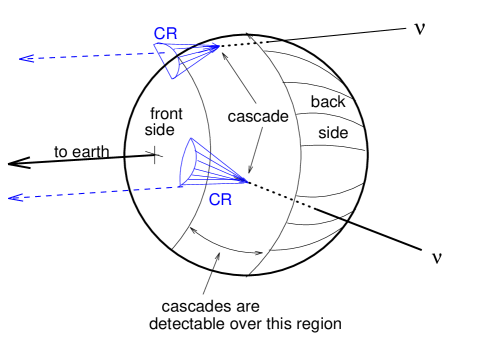
Figure 1: Schematic of the geometry for lunar neutrino cascade event detection.

At the regolith surface the resulting microwave Cherenkov radiation is refracted strongly into the forward direction. Scattering from surface irregularities and demagnification from the interface refraction gradient fills in the Cherenkov cone, and results in a larger effective area of the lunar surface over which events can be detected, as well as a greater acceptance solid angle. These effects are discussed in more detail in section III.A.

II.2 Antennas & receivers

The antennas employed in our search are the shaped-Cassegrainian 70 m antenna DSS14, and the beam waveguide 34 m antenna DSS13, both part of the NASA Goldstone Deep Space Network (DSN) Tracking Station. DSS13 is located about 22 km to the SSE of DSS14. The S-band (2.2 GHZ) right-circular-polarization (RCP) signal from DSS13 is filtered to 150 MHz BW, then downconverted with an intermediate frequency (IF) near 300 MHz. The band is then further subdivided into high and low frequency halves of 75 MHz each, and no overlap. These IF signals are then sent via an analog fiber-optic link to DSS14. At DSS14, the dual polarization S-band signals are downconverted with the same 300 MHz IF, and bandwidths of $100$ MHz (RCP) and 40 MHZ (LCP) are used. A third signal is also employed at DSS14: a 1.8 GHz (L-band) feed which is off-pointed by $\sim 0.5^{\circ}$ is used as a monitor of terrestrial interference signals; the signal is downconverted in the same manner as the other signals and has a 40 MHz bandwidth.

II.3 Trigger system

The experimental approach in our initial 12 hours of observations was to use a single antenna trigger with dual antenna data recording Gor99 . This was accomplished by using the local S-band signals as DSS14 to form a 2-fold coincidence with an active veto from the L-band interference monitor. Since any system with an active veto is subject to potential unforeseen impact on the trigger efficiency, we have now developed an approach which utilizes signals from both antennas to form a real-time dual-antenna trigger, with no active veto.

Fig. 2 shows the layout of the trigger. The four triggering signals from the two antennas are converted to unipolar pulses using tunnel-diode square-law detectors. Stanford Research Systems SR400 discriminators are used for the initial threshold level, and these are set to maintain a roughly constant singles rate, typically 0.5-1 kHz/chan for DSS14 and 30 kHz/chan for DSS13 (DSS13’s rate is higher due to a lower threshold, compensating for the reduced aperture size). A local coincidence is then formed for each antenna’s signals. The DSS14 coincidence between both circular polarizations ensures that the signals are highly linearly polarized, and the DSS13 coincidence helps to ensure that the signal is broadband.

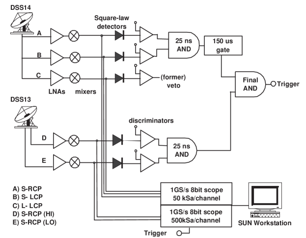
Figure 2: The GLUE trigger system used for the lunar neutrino search.

Fig. 3 indicates the timing sequence for a trigger to form (negative logic levels are used here). A local coincidence at DSS14, typically with a 25 ns gate, initiates the trigger sequence. After a 65 $\mu$s delay, a 150 $\mu$s gate is opened (the delays compensate for the 136 $\mu$s fiber delay between the two antennas). This large time window encompasses the possible geometric delay range for the moon throughout the year. Use of a smaller window is possible but would require delay tracking and a thus more stringent need for testing and reliability; use of a large window avoids this and a tighter coincidence can then be required offline.

If a 25 ns local coincidence now forms between the two DSS13 signals within the allowed 150 $\mu$s window, a trigger is formed. The sampling scopes are then triggered, and a 250 $\mu$s record, sampled at 1 Gs/s, is stored. The average trigger rate, due primarily to random coincidences of thermal noise fluctuations, is about 1.6 mHz, or 1 trigger every 5 minutes or so. Terrestrial interference triggers are uncommon (a few percent of the total), but can occasionally increase in number when a large burst of interference occurs at either antenna, with DSS14 more sensitive to this effect. The deadtime per event is about 6 s; thus on average we maintain about 99% livetime during a run.

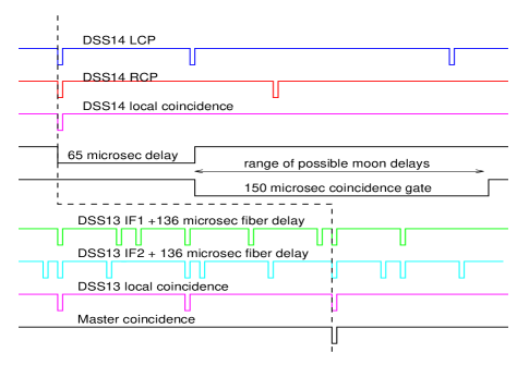
Figure 3: A timing diagram for the GLUE trigger system.

III Estimated sensitivity

Estimates of the sensitivity of radio telescope observations usually involve systems that integrate total power for some time constant $\Delta t$ which is in general much longer than the antenna’s single temporal mode duration which is given by the inverse of the bandwidth: $\tau=(\Delta\nu)^{-1}$. Since the pulses of interest in our experiment are much shorter than this time scale, the observed pulse structure of induced voltage in the antenna receiver is determined only by the bandpass function; that is, the pulses are band-limited. Thus the typical dependence of sensitivity on the factor $\sqrt{\Delta t\Delta\nu}$ does not obtain; this factor is always unity in band-limited pulse detection.

Because much of the theoretical work in describing such pulses has been done in terms of field strength rather than power, we analyze our sensitivity in these terms as well. Such analysis is also compatible with the receiving system, which records antenna voltages proportional to the incident electric field, and leads to a more linear analysis. It also yields signal-to-noise ratio estimates which are consistent with Gaussian statistics, since thermal noise voltages are described by a Gaussian random process.

The expected field strength per unit bandwidth from a cascade of total energy $W_{T}$ can be expressed as ZHS92 ; Alv96 ; Alv97 :

$$E_{0}~{}({\rm V~{}m^{-1}~{}MHz^{-1}})~{}=~{}{2.53\times 10^{-7}\over R}\left({W_{T}\over 1~{}{\rm TeV}}\right){\nu\over\nu_{0}}\left({1\over 1+0.4(\nu/\nu_{0})^{1.44}}\right)~{},$$ (2)

where $R$ is the distance to the source in m, $\nu$ is the radio frequency, and the decoherence frequency is $\nu_{0}\simeq 2500$ MHz for regolith material ($\nu_{0}$ scales mainly by radiation length). For typical parameters in our experiment, a $10^{19}$ eV cascade will result in a peak field strength at earth of $E\simeq 0.5~{}\mu$V m^-1 for a 70 MHz BW. Equation 2 has now been verified to within factors of $2$ through accelerator tests Gor00 ; Sal01 using silica sand targets and $\gamma$-ray-bunch-induced cascades with $W_{T}\leq 10^{19}$ eV per bunch.

Given that the use of a dual antenna trigger has virtually eliminated the problem of terrestrial interference that was the primary limitation to the sensitivity of the one previous experiment H96 , we can now express the minimum detectable field strength $E_{min}$ for each antenna in terms of the induced signal and the thermal noise background.

The expected signal strength $E_{0}$ induces a voltage at the antenna receiver given by

$$v_{s}~{}=~{}h_{e}E_{0}\Delta\nu$$ (3)

where the antenna effective height $h_{e}$ is given by Kra88

$$h_{e}~{}=~{}2\sqrt{{Z_{a}\eta A\over Z_{0}}}\cos\theta_{p}$$ (4)

where $Z_{a}$ is the antenna radiation resistance, $\eta$ and $A$ are the antenna efficiency and area, respectively, $Z_{0}=377~{}\Omega$ is the impedance of free space, and $\theta_{p}$ the polarization angle of the antenna with respect to the plane of polarization of the radiation.

The average thermal noise voltage in the system is given by

$$v_{n}~{}=~{}\sqrt{4kT_{sys}Z_{T}\Delta\nu}~{}.$$ (5)

Here $k$ is Boltzmann’s constant, $T_{sys}$ is the system thermal noise temperature, and $Z_{T}$ the termination impedance of the receiver. If we assume that $Z_{a}\approx Z_{T}$ then the resulting SNR $S$ is

$$S~{}\equiv~{}{v_{s}\over v_{n}}~{}=~{}E_{0}\cos\theta_{p}\sqrt{{\eta A\Delta\nu\over kT_{sys}Z_{0}}}~{}.$$ (6)

The minimum detectable field strength ($E_{0}\rightarrow E_{min}$) is then given by

$$E_{min}~{}=~{}S\sqrt{{kT_{sys}Z_{0}\over\eta A\Delta\nu}}~{}{1\over\cos\theta_{p}}~{}.$$ (7)

Combining this with equation 2 above, the threshold energy for pulse detection is

$$W_{thr}(\mbox{EeV})~{}\simeq~{}4.0\left({E_{min}\over{\rm 1V~{}m^{-1}MHz^{-1}}}\right)\left({R\over{\rm 1~{}m}}\right){\nu_{0}\over\nu}\left[{1+0.4\left({\nu\over\nu_{0}}\right)^{1.44}}\right]~{}.$$ (8)

For the lunar observations on the limb, which make up about 85% of the data reported here, $T_{sys}\simeq 110$ K, $\nu=2.2$ GHz, and the average $\Delta\nu\simeq 70$ MHz. For the 70 m antenna, with efficiency $\eta\simeq 0.8$, the minimum detectable field strength is $E_{min}\simeq 1.2\times 10^{-8}$ V m^-1 MHz^-1 for $\cos\theta_{p}=0.7$. The estimated threshold energy for these parameters is $W_{thr}=2.8\times 10^{19}$ eV, assuming a detection level of $S=5~{}(5\sigma)$ per IF at DSS14 (with a somewhat lower requirement at DSS13 in coincidence).

III.1 Monte Carlo results

To estimate the effective volume and acceptance solid angle as a function of incoming neutrino energy, events were generated at discrete neutrino energies, including the current best estimates of both charged and neutral current cross sections Gan00 , and the Bjorken-y distribution. Both electron and muon neutrino interactions were included, and Landau-Pomeranchuk-Migdal effects in the shower formation were estimated Alv97 . At each neutrino energy, a distribution of cascade angles and depths with respect to the local surface was obtained, and a refraction propagation of the predicted Cherenkov angular distribution was made through the regolith surface, including absorption and reflection losses and a first order roughness model. Antenna thermal noise fluctuations were included in the detection process.

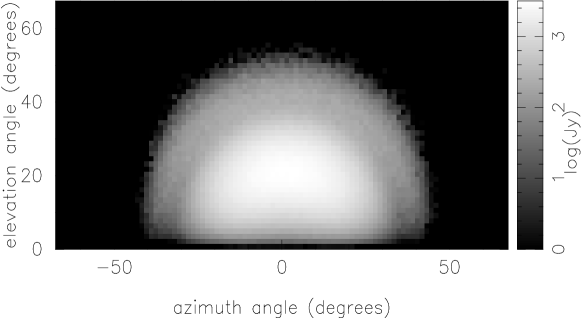
Figure 4: The microwave Cherenkov radiation pattern from an event in the lunar regolith.

A portion of the simulation is shown in Fig. 4. Here the flux density is shown as it would appear projected on the sky, with (0,0) corresponding to the tangent to the lunar surface in the direction of the original cascade. The units are Jy (1 Jy = $10^{-26}$ W m^-2 Hz^-1) as measured at earth, and the plot is an average over several hundred events at different depths and a range of $\theta_{up}$ consistent with a $10^{20}$ eV neutrino interaction, averaging over inelasticity effects and a mixture of electron and muon neutrinos consistent with decays from a hadronic $\pi^{\pm}$ source.

Although the averaging has broadened the distribution somewhat, a typical cascade still produces a flux density pattern of comparable angular size. The angular width of the pattern directly increases the acceptance solid angle, and the angular height increases the annular band of the lunar surface over which neutrino events can be detected, as indicated in Fig. 1. The net effect is that, although the specific flux density of the events are lowered somewhat by refraction and scattering, the effective volume and acceptance solid angle are significantly increased. The neutrino acceptance solid angle, in particular, is about a factor of 50 larger than the apparent solid angle of the moon itself.

III.2 EHE cosmic rays

We have noted above that the refraction geometry of the regolith favors emission from cascades that are upcoming relative to the local regolith surface. Thus to first order EHE cosmic ray events, which cascade within a few tens of cm as they enter the regolith, will not produce detectable pulses since their emission with be totally internally reflected within the regolith. This effect has been now demonstrated in an accelerator experiment Sal01 .

This conclusion does not account for several effects however. These effects are illustrated in Fig. 5. In Fig. 5A, the varying surface angles due surface roughness on scales greater than a wavelength will lead to escape of some radiation from cosmic ray cascades. Fig. 5B illustrates that, because the Cherenkov angular distribution is not infinitely narrow arround the Cherenkov angle (FWHM $\sim 1^{\circ}$), emission at angles larger then the Cherenkov angle can escape total internal reflectance. In Fig. 5C cascades from cosmic rays that enter along ridgelines can encounter a change in slope of the local surface that results in more efficient transmission of the radiation.

Even if total internal reflection strongly suppresses detection of cosmic rays in cases A and B, the latter case C of favorable surface geometry along ridgelines or hilltops will lead to some background of EHE cosmic ray events. We have not as yet made estimates of this background.

Fig. 5D shows the formation zone aspect of the process of Cherenkov emission from near-surface cosmic ray cascades. This constraint may suppress Cherenkov production even if surface roughness and the width of the Cherenkov distribution would otherwise favor some escape of emission.

Figure 5: Various effects associated with EHE cosmic ray hadron interactions.

It has now been conclusively shown Tak00 that coherent Cherenkov emission is a process involving the bulk dielectric properties of the radiating material. Cherenkov radiation is induced over a macroscopic region of the dielectric (with respect to the scale of a wavelength), and does not even require that the charged particles enter the dielectric for radiation to be produced—a proximity of several wavelengths or less is sufficient Ulr66 . A corollary to this result is that a cascade travelling along very near a boundary of the dielectric will not radiate (or radiate only weakly) into the hemisphere with the boundary.

Thus in the case of a cosmic ray entering the regolith at near grazing incidence (say within $\sim 1^{\circ}$) the resulting cascade reaches maximum within $\sim 3$ cm of the surface, still less than a wavelength for S-band observations. We therefore expect that the suppression of Cherenkov emission in such events significantly reduces our sensitivity to cosmic rays. Such effects have not been included yet in other estimates Alv96 ; Alv01 of the cosmic ray detection efficieny of such experiments.

IV Results

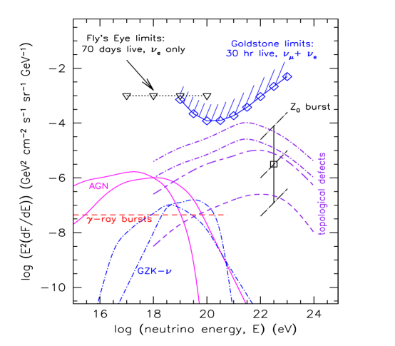
Figure 6: Plot of model neutrino fluxes and limits from the Fly’s Eye experiment and the present work.

Figure 6 plots the predicted fluxes of EHE neutrinos from a number of models including AGN production Man96 gamma-ray bursts BW99 , EHE cosmic-ray interactions HS85 , topological defects Yos97 ; Bha92 , and the $Z_{0}$ burst scenario Wei99 . Also plotted are limits from about 70 days of Fly’s Eye livetime Bal85 (accumulated in several years of runtime), which apply only to electron neutrino events.

Our initial 90% CL limit, for 30 hours of livetime is shown plotted with diamonds (see also Table 1), based on the observation of no events above an equivalent $5\sigma$ level amplitude (referenced to the 70 m antenna) consistent with the direction of the moon. These limits assume a monoenergetic signal at each energy; thus they are differential limits and independent of source spectral model, and represent the most conservative limits we can apply. Our limits just begin to constrain the highest topological defect model Yos97 for which we expected a total of order 1–2 events.

Table 1: Differential limits on mono-energetic EHE neutrino fluxes.

Energy (eV)	$10^{19}$	$3\times 10^{19}$	$10^{20}$	$3\times 10^{20}$	$10^{21}$	$3\times 10^{21}$	$10^{22}$	$3\times 10^{22}$	$10^{23}$
$\log_{10}(E^{2}dF/dE)$	-3.14	-3.66	-3.92	-3.91	-3.73	-3.42	-3.03	-2.66	-2.30
(GeV cm-2 s-1 sr-1)

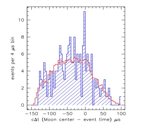
Figure 7: Low amplitude event histogram of GLUE data in delay with respect to the moon center delay. The overlain histogram is the expected background level. An excess occurs near zero delay, with a 2 microsecond offset.

In addition to the limits set above from the non-observation of events above, we have also analyzed events which triggered the system, but did not pass our more stringent software amplitude cuts. A sample of events was prepared by applying our standard cuts to remove terrestrial interference events. We required somewhat tighter timing that the hardware trigger, as well as band-limited pulse shape, but allowed smaller amplitudes, typically corresponding to $\sim 4.5\sigma$ at DSS14, and about $3\sigma$ at DSS13. The results are shown in Fig. 7, where the passing events have been binned according to their delay timing with respect to the expected delay from an event at the center of the moon. The background level (solid line) has been determined by randomizing the UT of the events and indicates the somewhat non-uniform seasonal coverage of our observations.

An excess is observed in the vicinity of zero delay where the lunar events are expected to cluster. At present there is a $\sim 2\mu$s offset from zero delay; this is too large to be accounted for by differential delays to the lunar limb, which can produce offsets of several hundred ns. Further study of the low amplitude events is in progress.

V Conclusions

We have developed a robust system for observing microwave pulses produced in the lunar regolith by electromagnetic particle cascades above $\sim 10^{19}$ eV. We have operated this system to achieve a livetime of 30 hours, with no large apparent signals detected to date. We have set conservative upper limits on the diffuse cosmic neutrino fluxes over the energy range from $10^{19-23}$ eV. We have also begun to analyze smaller events and have some preliminary indications that a signal may be present, but requiring further study.

We thank Michael Klein, George Resch, and the staff at Goldstone for their enthusiastic support of our efforts. This work was performed in part at the Jet Propulsion Laboratory, California Institute of Technology, under contract with NASA, and supported in part by the Caltech President’s Fund, by DOE contract DE-FG03-91ER40662 at UCLA, the Sloan Foundation, and the National Science Foundation.

References

- (1) P. W. Gorham, D. P. Saltzberg, P. Schoessow, et al., 2000, Phys. Rev. E. 62, 8590.
- (2) D. Saltzberg, P. Gorham, D. Walz, et al. 2001, Phys. Rev. Lett., in press.
- (3) G. A. Askaryan,1962, JETP 14, 441
- (4) G. A. Askaryan,1965, JETP 21, 658
- (5) I. M. Zheleznykh, 1988, Proc. Neutrino ’88, 528.
- (6) R. D. Dagkesamanskii, & I. M. Zheleznyk, 1989, JETP 50, 233
- (7) T. H. Hankins, R. D. Ekers & J. D. O’Sullivan, 1996, MNRAS 283, 1027.
- (8) E. Zas, F. Halzen,, & T. Stanev, 1992, Phys Rev D 45, 362
- (9) J. Alvarez–Muñiz, & E. Zas, 1996, Proc. 25th ICRC, ed. M.S. Potgeiter et al.,7,309.
- (10) J. Alvarez–Muñiz, & E. Zas, 1997, Phys. Lett. B, 411, 218
- (11) P. Gorham, et al., Proc. 26th ICRC, HE 6.3.15, astro-ph/9906504
- (12) D. Morrison & T. Own, 1987 The Planetary System, (Addison-Wesley: Reading,MA)
- (13) G. R. Olhoeft & D. W. Strangway, 1975, Earth Plan. Sci. Lett. 24, 394
- (14) J. D. Kraus, 1988, Antennas, (McGraw-Hill:New York)
- (15) R. Gandhi, 2000, hep-ph/0011176.
- (16) T. Takahashi, Y. Shibata, K. Ishi, et al. 2000, Phys Rev. E, 62, 8606
- (17) R. Ulrich, 1966, Zeit. Phys., 194, 180.
- (18) J. Alvarez–Muñiz, & E. Zas,, 2001, this proceedings.
- (19) E. Waxman & J. N. Bahcall,, 2000, Ap.J. 541, 707, astro-ph/9902383
- (20) Baltrusaitas, R.M., Cassiday, G.L., Elbert, J.W., et al 1985, Phys Rev D 31, 2192.
- (21) Bhattacharjee, P., Hill, C.T., & Schramm, D.N, 1992 PRL 69, 567.
- (22) Hill, C.T., & Schramm, D.N., 1985, Phys Rev D 31, 564.
- (23) Mannheim, K., 1996, Astropart. Phys 3, 295.
- (24) T. Weiler, 1999, hep-ph/9910316.
- (25) S. Yoshida, H. Dai, C. C. H. Jui, & P. Sommers, 1997, ApJ 479, 547.