Scalar Field Dark Matter

Abstract

This work is a review of the last results of research on the Scalar Field Dark Matter model of the Universe at cosmological and at galactic level. We present the complete solution to the scalar field cosmological scenario in which the dark matter is modeled by a scalar field $\Phi$ with the scalar potential $V(\Phi)=V_{0}\left[\cosh{(\lambda\,\sqrt{\kappa_{0}}\Phi)}-1\right]$ and the dark energy is modeled by a scalar field $\Psi$, endowed with the scalar potential $\tilde{V}(\Psi)=\tilde{V_{0}}\left[\sinh{(\alpha\,\sqrt{\kappa_{0}}\Psi)}\right]^{\beta}$, which together compose the $95\%$ of the total matter energy in the Universe. The model presents successfully deals with the up to date cosmological observations, and is a good candidate to treat the dark matter problem at the galactic level.

I Introduction

There is no doubt that we are living exiting times in physics. Certainly, the last results of the observations of the Universe will conduce to a qualitative new knowledge of Nature. One question which singles out is that of finding out which is the nature of the matter energy composing the Universe. It is amazing that after so much effort dedicated to such a question, what is the Universe composed of?, it has not been possible to give a conclusive answer. From the latest observations, we do know that about 95% of matter in the Universe is of non baryonic nature. The old belief that matter in Cosmos is made of quarks, leptons and gauge bosons is being abandoned due to the recent observations and the inconsistencies which spring out of this assumption [1]. We think there is strong evidence on the existence of an exotic non baryonic sort of matter which dominates the structure of the Universe, but its nature is until now a puzzle.

In this work we pretend to summarize the results of one proposal for the nature of the matter in the Universe, namely, the Scalar Field Dark Matter model (SFDM). This model has had relative success at cosmological level as well as at galactic scale. In this work we pretend to put both models together and explain which is the possible connection between them.

The hypothesis that the scalar field is the dark matter is not new. For example, Denhen has proposed that the Higgs scalar field could be the dark matter in galaxies [2, 3]. Other authors has suggested that the halo of galaxies are boson stars, etc. Maybe the most popular hypothesis was the axions fields as dark matter. Nevertheless, this hypothesis show some problems of consistency[4, 5]. In our opinion, it was not possible to do a model of the Universe till the accelerated expansion of it was established. Most of the material contained in this work has been separately published elsewhere, the main goal of this work is to write it all together and with a unifying description. First, let us give a brief introduction of the Dark Matter problem.

The existence of dark matter in the Universe has been firmly established by astronomical observations at very different length-scales, ranging from single galaxies, to clusters of galaxies, up to cosmological scale (see for example [6]). A large fraction of the mass needed to produce the observed dynamical effects in all these very different systems is not seen. At the galactic scale, the problem is clearly posed: The measurements of rotation curves (tangential velocities of objects) in spiral galaxies show that the coplanar orbital motion of gas in the outer parts of these galaxies keeps a more or less constant velocity up to several luminous radii [7, 8], forming a nearly radii independent curve in the outer parts of the rotational curves profile; a motion which does not correspond to the one due to the gravitational effects of the observed matter distribution, hence there must be present some type of dark matter causing the observed motion. The flat profile of the rotational curves is the clearest indication of the presence of more than the observed matter. It is usually assumed that the dark matter in galaxies has an almost spherical distribution which decays like $1/r^{2}$. With this distribution of some kind of matter it is possible to fit the rotational curves of galaxies quite well [8]. Nevertheless, the main question of the dark matter problem remains: Which is the nature of the dark matter in the Universe? The problem is not easy to solve, it is not sufficient to find out an exotic particle which could exist in galaxies in the low energy regime of some theory. It is necessary to show as well, that this particle distributes in a very similar manner in all these galaxies, and finally, to give even some reason for its existence in galaxies.

Recent observations of the luminosity-redshift relation of Ia Supernovae suggest that distant galaxies are moving slower than predicted by Hubble’s law impliying an accelerated expansion of the Universe [9]. These observations open the possibility to the existence of an energy component in the Universe with a negative equation of state, $\omega<0$, being $p=\omega\rho$, called dark energy. This result is very important because it separates the components of the Universe into gravitational (also called the “matter component” of the Universe) and antigravitational (repulsive, the dark energy). The dark energy would be the currently dominant component in the Universe and its ratio relative to the whole energy would be $\Omega_{DE}\sim 70\%$. The most simple model for this dark energy is the cosmological constant ($\Lambda$), for which $\omega=-1$.

Observations in galaxy clusters and dynamical measurements of the mass in galaxies indicate that the matter component of the Universe is $\Omega_{M}\sim 30\%.$ But this component of the Universe decomposes itself in baryons, neutrinos, etc. and cold dark matter, which is the responsible of the formation of structure in the Universe. Observations indicate that stars and dust (baryons) represent something like $0.3\%$ of the whole matter of the Universe. The new measurements of the neutrino mass indicate that neutrinos contribute with a same quantity like dust. In other words, say $\Omega_{M}=\Omega_{b}+\Omega_{\nu}+\cdot\cdot\cdot+\Omega_{DM}\sim 0.05+\Omega_{DM}$, where $\Omega_{DM}$ represents the dark matter part of the matter contributions which has a value of $\Omega_{DM}\sim 0.25$. The value of the amount of baryonic matter ($\sim 5\%$) is in concordance with the bounds imposed by nucleosynthesis (see for example [1]). These observations are in very good agreement with the preferred value $\Omega_{0}\sim 1.$

The standard cosmological model then considers a flat Universe ($\Omega_{\Lambda}+\Omega_{M}\approx 1$) full with $95\%$ of unknown matter which is of great importance at cosmological level. Moreover, it seems to be the most successful model fitting current cosmological observations [10].

The SFDM model [11, 12, 13, 14] consists in to assume that the dark matter and the dark energy are of scalar field nature. A particular model we have considered in the last years is the following. For the dark energy we adopt a quintessence field ${\Psi}$ with a $\sinh$ like scalar potential. In [15], it was showed that the potential

$$\tilde{V}(\Psi) = \tilde{V_{0}}\left[\sinh{(\alpha\,\sqrt{\kappa_{0}}\Psi)}\right]^{\beta}$$ (1)

$$= \left\{\begin{array}[]{cc}\tilde{V_{0}}\left(\alpha\,\sqrt{\kappa_{0}}\Psi\right)^{\beta}&|\alpha\,\sqrt{\kappa_{0}}\Psi|\ll 1\\ \left(\tilde{V_{0}}/2^{\beta}\right)\exp{\left(\alpha\beta\,\sqrt{\kappa_{0}}\Psi\right)}&|\alpha\,\sqrt{\kappa_{0}}\Psi|\gg 1\end{array}\right.;$$ (4)

is a reliable model for the dark energy, because of its asymptotic behaviors. Nevertheless, the main point of the SFDM model is to suppose that the dark matter is a scalar field ${\Phi}$ endowed with the potential [14]

$$V(\Phi) = V_{0}\left[\cosh{(\lambda\,\sqrt{\kappa_{0}}\Phi)}-1\right]$$ (5)

$$= \left\{\begin{array}[]{cc}\frac{1}{2}m^{2}_{\Phi}\Phi^{2}+\frac{1}{24}\lambda^{2}m^{2}_{\Phi}\kappa_{0}\Phi^{4}&|\lambda\,\sqrt{\kappa_{0}}\Phi|\ll 1\\ \left(V_{0}/2\right)\exp{\left(\lambda\,\sqrt{\kappa_{0}}\Phi\right)}&|\lambda\,\sqrt{\kappa_{0}}\Phi|\gg 1\end{array}\right..$$ (8)

The mass of the scalar field $\Phi$ is defined as $m_{\Phi}^{2}=V^{\prime\prime}|_{\Phi=0}=\lambda^{2}\kappa_{0}V_{0}$. In this case, we are dealing with a massive scalar field.

The main results of the model presented in this work are: 1) the fine tuning and the cosmic coincidence problems are ameliorated for both dark matter and dark energy and the models agrees with astronomical observations. 2) The model predicts a suppression of the Mass Power Spectrum for small scales having a wave number $k>k_{min,\Phi}$, where $k_{min,\Phi}\simeq 4.5\,h\,$ Mpc^-1 for $\lambda\simeq 20.3$. This last fact could help to explain the dearth of dwarf galaxies and the smoothness of galaxy core halos. 3) From this, all parameters of the scalar dark matter potential are completely determined. 4) The dark matter consists of an ultra-light particle, whose mass is $m_{\Phi}\simeq 1.1\times 10^{-23}\,{\rm eV}$ and all the success of the standard cold dark matter model is recovered. 5) If the scale of renormalization of the model is of order of the Planck Mass, then the scalar field $\Phi$ can be a reliable model for dark matter in galaxies. 6) The predicted scattering cross section fits the value required for self-interacting dark matter. 7) Studying a spherically symmetric fluctuation of the scalar field $\Phi$ in cosmos we show that it could be the halo dark matter in galaxies. 8) The local space-time of the fluctuation of the scalar field $\Phi$ contains a three dimensional space-like hypersurface with surplus of angle. 9) We also present a model for the dark matter in the halos of spiral galaxies, we obtain that the effective energy density goes like $1/(r^{2}+K^{2})$ and 10) the resulting circular velocity profile of tests particles is in good agreement with the observed one in spiral galaxies.

All these facts lead us to consider that the scalar field is a very good candidate for being the dark matter of the Universe.

II Cosmological Scalar Field Solutions

In this section, we give all the solutions to the model at the cosmological scale and focus our attention in the scalar dark matter. Since current observations of CMBR anisotropy by BOOMERANG and MAXIMA [16] suggest a flat Universe, we use as ansatz the flat Friedmann-Robertson-Walker (FRW) metric

$$ds^{2}=-dt^{2}+a^{2}(t)\left[dr^{2}+r^{2}d\Omega^{2}\right],$$ (9)

where $a$ is the scale factor ($a=1$ today) and we have set $c=1$. The components of the Universe are baryons, radiation, three species of light neutrinos, etc., and two minimally coupled and homogenous scalar fields $\Phi$ and $\Psi$, which represent the dark matter and the dark energy, respectively. The evolution equations for this Universe read

$$H^{2}\equiv\left(\frac{\dot{a}}{a}\right)^{2} = \frac{\kappa_{0}}{3}\left(\rho+\rho_{\Phi}+\rho_{\Psi}\right)$$ (10)

$$\ddot{\Phi}+3H\dot{\Phi}+\frac{dV(\Phi)}{d\Phi} = 0$$ (11)

$$\ddot{\Psi}+3H\dot{\Psi}+\frac{d\tilde{V}(\Psi)}{d\Psi} = 0$$ (12)

$${\dot{\rho}}+3H\left(\rho+p\right) = 0,$$ (13)

being $\kappa_{0}\equiv 8\pi G$ and $\rho$ ($p$) is the energy density (pressure) of radiation, plus baryons, plus neutrinos, etc. The scalar energy densities (pressures) are $\rho_{\Phi}=\frac{1}{2}\dot{\Phi}^{2}+V(\Phi)$ ($p_{\Phi}=\frac{1}{2}\dot{\Phi}^{2}-V(\Phi)$) and $\rho_{\Psi}=\frac{1}{2}\dot{\Psi}^{2}+\tilde{V}(\Psi)$ ($p_{\Psi}=\frac{1}{2}\dot{\Psi}^{2}-\tilde{V}(\Psi)$). Here overdots denote derivative with respect to the cosmological time $t$.

A Radiation Dominated Era (RD)

We start the evolution of the Universe at the end of inflation, $i.e.$ in the radiation dominated (RD) era. The initial conditions are set such that $\left(\rho_{i\Phi},\,\rho_{i\Psi}\right)\leq\rho_{i\gamma}$. Let us begin with the dark energy. For the potential (1) an exact solution in the presence of nonrelativistic matter can be found[15, 17] and the parameters of the potential are given by

$$\alpha = \frac{-3\omega_{\Psi}}{2\sqrt{3(1+\omega_{\Psi})}},$$ (14)

$$\beta = \frac{2\,(1+\omega_{\Psi})}{\omega_{\Psi}},$$ (15)

$$\kappa_{0}\tilde{V_{0}} = \frac{3(1-\omega_{\Psi})}{2}\left(\frac{\Omega_{oM}}{\Omega_{o\Psi}}\right)^{\frac{1+\omega_{\Psi}}{\omega_{\Psi}}}\Omega_{o\Psi}H^{2}_{0}$$ (16)

with $\Omega_{o\Psi}$ and $\Omega_{oCDM}$ the current values of dark energy and dark matter, respectively; and $-0.9\leq\omega_{\Psi}\leq-0.6$ the range for the current equation of state. With these values for the parameters ($\alpha,\,\beta<0$) the solution for the dark energy ($\Psi$) becomes a tracker one and is only reached until a matter dominated epoch. The scalar field $\Psi$ would begin to dominate the expansion of the Universe after matter domination. Before this, at the radiation dominated epoch, the scalar energy density $\rho_{\Psi}$ is frozen, strongly subdominant and of the same order than today [15]. Then the dark energy contribution can be neglected during this epoch.

Now we study the behavior of the dark matter. For the potential (5) we begin the evolution with large and negative values of $\Phi$, when the potential behaves as an exponential one. It is found that the exponential potential makes the scalar field $\Phi$ mimic the dominant energy density, that is, $\rho_{\Phi}=\rho_{i\Phi}a^{-4}$. The ratio of $\rho_{\Phi}$ to the total energy density is [17, 18]

$$\frac{\rho_{\Phi}}{\rho_{\gamma}+\rho_{\Phi}}=\frac{4}{\lambda^{2}}.$$ (17)

This solution is self-adjusting and it helps to avoid the fine tuning problem of matter, too. Here appears one restriction due to nucleosynthesis [18] acting on the parameter $\lambda>\sqrt{24}$. Once the potential (5) reaches its polynomial behavior, $\Phi$ oscillates so fast around the minimum of the potential that the Universe is only able to feel the average values of the energy density and pressure in a scalar oscillation. Both $\Phi$ and $<\omega_{\Phi}>$ go down to zero and $<\rho_{\Phi}>$ scales as non-relativistic matter [19]. If we would like the scalar field $\Phi$ to act as cold dark matter, in order to recover all the successful features of the standard model, we need first derive a relation between the parameters ($V_{0}$, $\lambda$). The required relation reads [14]

$$\kappa_{0}V_{0}\simeq\frac{1.7}{3}\left(\lambda^{2}-4\right)^{3}\left(\frac{\Omega_{0CDM}}{\Omega_{o\gamma}}\right)^{3}\Omega_{0CDM}H^{2}_{0}.$$ (18)

Notice that $V_{0}$ depends on both current amounts of dark matter and radiation (including light neutrinos) and that we can choose $\lambda$ to be the only free parameter of potential (5). Since now, we can be sure that $\rho_{\Phi}=\rho_{CDM}$ and that we will recover the standard cold dark matter evolution.

B Matter Dominated Era (MD) and Scalar Field $\Psi$ Dominated Era ($\Psi$D)

During this time, the scalar field $\Phi$ continues oscillating and behaving as nonrelativistic matter and there is a matter dominated era just like that of the standard model. A short after matter completely dominates the evolution of the Universe, the scalar field $\Psi$ reaches its tracker solution and it begins to be an important component. Lately, the scalar field $\Psi$ becomes the dominant componente of the Universe and the scalar potential (1) is effectively an exponential one [13, 15]. Thus, the scalar field $\Psi$ drives the Universe into a power-law inflationary stage ($a\sim t^{p}$, $p>1$). This solution is distinguishable from a cosmological constant one [15].

A complete numerical solution for the dimensionless density parameters $\Omega$’s are shown in Fig. 1 up to date. The results agree with the solutions found in this section. It can be seen that eq. (18) makes the scalar field $\Phi$ behave quite similar to the standard cold dark matter model once the scalar oscillations start and the required contributions of dark matter and dark energy are the observed ones [14, 15, 20]. We recovered the standard cosmological evolution and then we can see that potentials (1,5) are reliable models of dark energy and dark matter in the Universe.

FIG. 1.: Evolution of the dimensionless density parameters vs the scale factor $a$ with $\Omega_{oM}=0.30$: $\Lambda$CDM (solid-curves) and $\Psi\Phi DM$ for two values of $\lambda=6$ (dashed-curves), $\lambda=8$ (dotted-curves). The equation of state for the dark energy is $\omega_{\Psi}=-0.8$.

C Scalar Power Spectrum for $\Phi$ dark matter

In this section, we analyze the perturbations of the space due to the presence of the scalar fields $\Phi,\Psi$. First, we consider a linear perturbation of the space given by $h_{ij}$. We will work in the synchronous gauge formalism, where the line element is $ds^{2}=a^{2}[-d\tau^{2}+(\delta_{ij}+h_{ij})dx^{i}dx^{j}]$. We must add the perturbed equations for the scalar fields $\Phi(\tau)\rightarrow\Phi(\tau)+\phi(k,\tau)$ and $\Psi(\tau)\rightarrow\Psi(\tau)+\psi(k,\tau)$[18, 21]

$$\ddot{\phi}+2{\cal H}\dot{\phi}+k^{2}\phi+a^{2}V^{\prime\prime}\phi+\frac{1}{2}\dot{\Phi}\dot{h} = 0$$ (19)

$$\ddot{\psi}+2{\cal H}\dot{\psi}+k^{2}\psi+a^{2}\tilde{V}^{\prime\prime}\psi+\frac{1}{2}\dot{\Psi}\dot{h} = 0.$$ (20)

to the linearly perturbed Einstein equations in $k$-space ($\vec{k}=k\hat{k}$) (see [22]). Here, overdots are derivatives with respect to the conformal time $\tau$ and primes are derivatives with respect of the unperturbed scalar fields $\Phi$ and $\Psi$, respectively.

It is known that scalar perturbations can only grow if the $k^{2}$-term in eqs. (19,20) is subdominant with respect to the second derivative of the scalar potential, that is, if $k<a\sqrt{V^{\prime\prime}}$ [23]. According to the solution given above for potential (5), $k_{\Phi}=a\sqrt{V^{\prime\prime}}$ has a minimum value given by [20]

$$k_{min,\Phi}=m_{\Phi}a^{\ast}\simeq 1.3\,\lambda\sqrt{\lambda^{2}-4}\frac{\Omega_{0CDM}}{\sqrt{\Omega_{o\gamma}}}H_{0},$$ (21)

$a^{\ast}$ being the scale factor at the time when the scalar field $\Phi$ starts to oscillate coherently around the minimum of the scalar potential (5). For $\lambda\geq 5$, we have that $k_{min,\Phi}\geq 0.375\,$ Mpc^-1. Then, it can be assured that there are no scalar perturbations for $k>m_{\Phi}$, that is, bigger than $k_{\Phi}$ today. These $k$ correspond to scales smaller than $1.2$ kpc (here $\lambda=5$). They must have been completely erased. Besides, modes which $m_{\Phi}>k>k_{min,\Phi}$ must have been damped during certain periods of time. From this, we conclude that the scalar power spectrum of $\Phi$ will be damped for $k>k_{min,\Phi}$ with respect to the standard case. Therefore, the Jeans length must be [20]

$$L_{J}(a)=2\pi\,k^{-1}_{min,\Phi},$$ (22)

and it is a universal constant because it is completely determined by the mass of the scalar field particle. $L_{J}$ is not only proportional to the quantity $(\kappa_{0}V_{0})^{-1/2}$ (recalling that $m^{2}_{\Phi}=\lambda^{2}\kappa_{0}V_{0}$), but also the time when scalar oscillations start (represented by $a^{\ast}$) is important.

On the other hand, the wave number for the dark energy $k_{\Psi}=a\sqrt{\tilde{V}^{\prime\prime}}$ is always out of the Hubble horizon, then only structure at larger scales than $H^{-1}$ can be formed by the scalar fluctuations $\psi$. Instead of a minimum, there is a maximum $k_{max,\Psi}\sim 10^{-3}\,$ Mpc^-1. All scalar perturbations of the dark energy which $k>10^{-3}\,$ Mpc^-1 must have been completely erased. Perturbations with $k\leq 10^{-3}\,$ Mpc^-1 have started to grow only recently. For a more detailed analysis of the dark energy fluctuations, see [23, 24].

In Fig. 2, a numerical evolution of the density contrasts $\delta\equiv\delta\rho/\rho$ is shown compared with the standard CDM case[14]. The evolution was done using an amended version of CMBFAST [25]. Due to its oscillations around the minimum, the scalar field $\Phi$ changes to a complete standard CDM and so do its perturbations. All the standard growing behavior for modes $k<k_{min,\Phi}$ is recovered and preserved until today by potential (5).

FIG. 2.: Evolution of the density contrasts for baryons $\delta_{b}$, standard cold dark matter $\delta_{CDM}$ and scalar dark matter $\delta_{\Phi}$ vs the scale factor $a$ taking $\Omega_{oM}=0.30$ for the models given in fig. (1). The modes shown are $k=1.0\times 10^{-5}\,$ Mpc^-1 (left) and $k=0.1\,$ Mpc^-1 (right).

In Fig. 3 we can see $\delta^{2}$ at a redshift $z=50$ from a complete numerical evolution using the amended version of CMBFAST[20].We also observe a sharp cut-off in the processed power spectrum at small scales when compared to the standard case, as it was argued above. This suppression could explain the smooth cores of dark halos in galaxies and a less number of dwarf galaxies [26].

FIG. 3.: Power spectrum at a redshift $z=50$: $\Lambda$CDM (solid-curve), and $\Phi$CDM with $\lambda=5$ (dashed-curve) and $\lambda=10$ (dotted-curve). The normalization is arbitrary.

The mass power spectrum is related to the CDM case by the semi-analytical relation (see [27])

$$P_{\Phi}(k)\simeq\left(\frac{\cos{x^{3}}}{1+x^{8}}\right)^{2}P_{CDM}(k),$$ (23)

but using $x=(k/k_{min,\Phi})$ with $k_{min,\Phi}$ being the wave number associated to the Jeans lenght (22). If we take a cut-off of the mass power spectrum at $k=4.5\,h\,{\rm Mpc}^{-1}$ [26], we can fix the value of parameter $\lambda$. Using eq. (21), we find that [20]

$$\lambda \simeq 20.3,$$ (24)

$$V_{0} \simeq \left(3.0\times 10^{-27}\,M_{Pl}\simeq 36.5\,{\rm eV}\right)^{4},$$ (25)

$$m_{\Phi} \simeq 9.1\times 10^{-52}\,M_{Pl}\simeq 1.1\times 10^{-23}\,{\rm eV}.$$ (26)

where $M_{Pl}=1.22\times 10^{19}\,{\rm GeV}$ is the Plank mass. All parameters of potential (5) are now completely determined and we have the right cut-off in the mass power spectrum.

III Scalar dark matter and Planck scale physics

At galactic scale, numerical simulations show some discrepancies between dark-matter predictions and observations [28]. Dark matter simulations show cuspy halos of galaxies with an excess of small scale structure, while observations suggest a constant halo core density [29] and a small number of subgalactic objects [30]. There have been some proposals for resolving the dark matter crisis (see for example [28, 30]). A promising model is that of a self-interacting dark matter [31]. This proposal considers that dark matter particles have an interaction characterized by a scattering cross section by mass of the particles given by [29, 31]

$$\frac{\sigma_{2\rightarrow 2}}{m}=10^{-25}-10^{-23}cm^{2}\,GeV^{-1}.$$ (27)

This self-interaction provides shallow cores of galaxies and a minimum scale of structure formation, that it must also be noticed as a cut-off in the Mass Power Spectrum [26, 30].

Because of the presence of the scalar field potential (5), there must be an important self-interaction among the scalar particles. That means that this scalar field dark matter model belongs to the so called group of self-interacting dark matter models mentioned above, and it should be characterized by the scattering cross section (27).

Let us calculate $\sigma_{2\rightarrow 2}/m_{\Phi}$ for the scalar potential (5). The scalar potential (5) can be written as a series of even powers in $\Phi$, $V=\sum_{n=1}^{\infty}V_{0}\lambda^{2n}\kappa_{0}^{n}\Phi^{2n}$. Working on 4 dimensions, it is commonly believed that only $\Phi^{4}$ and lower order theories are renormalizable. But, following the important work [32], if we consider that there is only one intrinsic scale $\Lambda$ in the theory, we conclude that there is a momentum cut-off and that we can have an effective $\Phi^{4}$ theory which depends upon all couplings in the theory. In addition, it was recently demonstrated [33] that scalar exponential-like potentials of the form (we have used the notation of potential (5) and for example, parameter $\mu$ in eqs. (7-8) in ref. [33] is $\mu^{-1}=\lambda\sqrt{\kappa_{0}}$)) [34]

$$U_{\Lambda}(\Phi)=M^{4}\exp{\left(-\frac{\lambda^{2}\kappa_{0}\Lambda^{2}}{32\pi^{2}}\right)}\exp{\left(\pm\lambda\sqrt{\kappa_{0}}\Phi\right)}$$ (28)

are non-perturbative solutions of the exact renormalization group equation in the Local Potential Approximation (LPA). Here $M$ and $\lambda$ are free parameters of the potential and $\Lambda$ is the scale of renormalization. Being our potential for scalar dark matter a $\cosh$-like potential (non-polynomial), it is then a solution to the renormalization group equations in the (LPA), too. Comparing eqs. (5, 28), we can identify $V_{0}=M^{4}\exp{\left[-\left(\lambda^{2}\kappa_{0}\Lambda^{2}\right)/(32\pi^{2})\right]}$. We see that an additional free parameter appears, the scale of renormalization $\Lambda$. From this, we can assume that potential (5) is renormalizable with only one intrinsic scale: $\Lambda$.

Following the procedure shown in [35] for a potential with even powers of the dimensionless scalar field $\phi$, $U(\phi)=\sum^{\infty}_{n=1}u_{2n}\phi^{2n}$, the cross section for $2\rightarrow 2$ scattering in the center-of-mass frame is [34]

$$\sigma_{2\rightarrow 2}=\frac{M^{8}\kappa^{4}_{0}\lambda^{8}}{16\pi E^{2}},$$ (29)

where $E$ is the total energy. Thus, we arrive to a real effective $\phi^{4}$ theory with a coupling $g=M^{4}\kappa^{2}_{0}\lambda^{4}$, leading to a different cross section for the self-interacting scalar field than that obtained from polynomial models [36]. Near the threshold $E\simeq 4m^{2}$, and taking the values of $\lambda$, $m_{\Phi}$ and the expected result (27), we find $M=(6.7\pm 1.9)\times 10^{2}$ TeV and $\Lambda\simeq(1.93\pm 0.01)\,M_{Pl}\simeq 2.3\times 10^{19}$ GeV. The scale of renormalization is of order of the Planck Mass. All parameters are completely fixed now [34].

IV Scalar Field Dark Matter in Galaxies

In this section we explore whether a scalar field can fluctuate along the history of the Universe and thus forming concentrations of scalar field density. This idea was first explored in the early 90’s for a Bose gas made of Higgs bosons in the newtonian regime [2, 3, 37]. Nevertheless, we assume that the halo of a galaxy is a fluctuation of cosmological scalar dark matter and study the consequences for the space-time background at this scale starting directly from a relativistic point of view [38]. Such relativistic approach for weakly gravitating systems has its origins in the Projective Unified Field Theory [39, 40], where it appears a scalar field as a consequence of the projection to four dimensions.

The region of the galaxy we are interested in is that which goes from the limits of the luminous matter (including the stars far away of the center of the galaxy) over the limits of the halo. In this region measurements indicate that circular velocity of stars is almost independent of the radii at which they are located within the equatorial plane [41]. Observational data show that the galaxies are composed by almost 90% of dark matter. Nevertheless the halo contains a larger amount of dark matter, because otherwise the observed dynamics of particles in the halo is not consistent with the predictions of Newtonian theory, which explains well the dynamics of the luminous sector of the galaxy. So we can suppose that luminous matter does not contribute in a very important way to the total energy density of the halo of the galaxy at least in the mentioned region, instead the scalar matter will be the main contributor to it. As a first approximation we can neglect the baryonic matter contribution to the total energy density of the halo of the galaxy. On the other hand, the exact symmetry of the halo is stills unknown, but it is reasonable to suppose that the halo is symmetric with respect to the rotation axis of the galaxy. Furthermore, the rotation of the galaxy does not affect the motion of test particles around the galaxy, dragging effects in the halo of the galaxy should be too small to affect the tests particles (stars) traveling around the galaxy. Hence, we can consider a time reversal symmetry of the space-time. We consider that the dark matter will be the main contributor to the dynamics, and then we will treat the observed luminous matter as a test fluid. The line-element of such space-time, given in the Papapetrou form is [42]:

$$ds^{2}=-e^{2\,\psi}(dt+\omega\,d\varphi)^{2}+e^{-2\psi}[e^{2\gamma}(d\rho^{2}+dz^{2})+\mu^{2}d\varphi^{2}],$$ (30)

where $\psi,\omega,\gamma$, and $\mu$, are functions of $(\rho,z)$.

We will derive the geodesic equations in the equatorial plane, that is for $z=\dot{z}=0$, where dot stands for the derivative with respect to the proper time $\tau$. The Lagrangian for a test particle travelling on the static space time ($\omega=0$) described by (30) is given by:

$$2{\cal L}=-e^{2\,\psi}\dot{t}^{2}+e^{-2\psi}[e^{2\gamma}\,(\dot{\rho}^{2}+\dot{z}^{2})+\mu^{2}\,\dot{\varphi}^{2}],$$ (31)

In order to have stable circular motion, which is the motion we are interested in, we have to satisfy three conditions:

i) $\dot{\rho}=0$, and

ii)${\frac{{\partial V(\rho)}}{{\partial\,\rho}}}=0$, where $V(\rho)=-e^{2(\psi-\gamma)}\,[E\,\dot{t}-L\,\dot{\varphi}-1]$.

iii)${\frac{{\partial^{2}V(\rho)}}{{\partial\,\rho^{2}}}}|_{extr}>0$, in order to have a minimum.

Under these conditions, we find the form of the line element in the equatorial plane has to be [43]

$$ds^{2}=-\left({\frac{{\mu}}{{\mu_{0}}}}\right)^{2l}\,dt^{2}+\left({\frac{{\mu}}{{\mu_{0}}}}\right)^{-2l}\,[e^{2\,\gamma}\,d\rho^{2}+\mu^{2}\,d{\varphi}^{2}].$$ (32)

where $l=(v^{\varphi})^{2}/(1+(v^{\varphi})^{2})$, being $v^{\varphi}$ the tangential velocity of a test particle travelling on the equatorial plane of the background space-time. Notice that this type of space time definitely can not be asymptotically flat.

In what follows we study the circular trajectories of a test particle on the equatorial plane taking the space-time (32) as the background. The motion equation of a test particle in such space-time can be derived from the Lagrangian (31), the angular momentum per unit of mass is

$$\frac{\mu^{2}}{f}\frac{d\varphi}{d\tau}=B,$$ (33)

where $f=e^{2\psi}=\left({\mu/\mu_{0}}\right){{}^{2l}}$ and the total energy of the test particle reads

$$f\ c^{2}\frac{d\ t}{d\tau}=A,$$ (34)

with $\tau$ is the proper time of the test particle. An observer falling freely into the galaxy, with coordinates $(\rho,\zeta,\phi,t)$, will have a line element given by

$$ds^{2} = \left\{\frac{1}{f\ c^{2}}[e^{2\gamma}({\dot{\rho}}^{2}+{\dot{\zeta}}^{2})+\mu^{2}{\dot{\varphi}}^{2}]-f\right\}c^{2}dt^{2}$$ (35)

$$= \left(\frac{v^{2}}{c^{2}}-f\right)c^{2}dt^{2}$$ (36)

$$= -c^{2}d\tau^{2}.$$ (37)

The velocity ${\bf v}$ given by $v^{a}=(\dot{\rho},\dot{\zeta},\dot{\phi})$, is the three-velocity of the test particle, where a dot means derivative with respect to $t$, the time measured by the free falling observer. The squared velocity $(v^{\varphi})^{2}$ is

$$v^{2}=g_{ab}v^{a}v^{b}=\frac{e^{2\gamma}}{f}(\dot{\rho}^{2}+\dot{\zeta}^{2})+\frac{\mu^{2}}{f}\dot{\varphi}^{2},$$ (38)

where $a,b=1,2,3$. Using equation (36) we obtain an expression for $dt/d\tau$, by substituting it into (34), we get

$$A^{2}=\frac{c^{4}f^{2}}{f-\frac{v^{2}}{c^{2}}}.$$ (39)

For the axisymmetric scalar field dark matter halo, an exact solution of the field equations reads in Boyer-Lindquist coordinates [12]:

$$ds^{2} = -f_{0}c^{2}\left(r^{2}+b^{2}\sin^{2}{\theta}\right)dt^{2}$$ (42)

$$+\frac{1+b^{2}\cos^{2}{\theta}/r^{2}}{f_{0}}\left(\frac{dr^{2}}{1+b^{2}/r^{2}}+r^{2}d\theta^{2}\right)$$

$$+\frac{r^{2}+b^{2}\sin^{2}{\theta}}{f_{0}}d\varphi^{2}$$

and the effective energy density $\mu_{DM}$ is half the value of the scalar potential:

$$\mu_{DM} = \frac{1}{2}V(\Phi)=-\frac{2f_{0}r_{0}}{\kappa_{0}(r^{2}+b^{2}\sin^{2}{\theta)}},$$ (43)

$$V(\Phi) = -\frac{l}{\kappa_{0}(1-l)}exp\left[-2\sqrt{\frac{\kappa_{0}}{l}}(\Phi-\Phi_{0})\right]$$ (44)

being $\mu=\sqrt{r^{2}+b^{2}}\sin\theta$ and $\zeta=r\cos\theta$ in (32).

The geodesic equations of the metric (42) in the equatorial plane read

$$\frac{d^{2}D}{d\tau^{2}}-D\left(\frac{d\varphi}{d\tau}\right)^{2}+f_{0}^{2}c^{2}D\left(\frac{dt}{d\tau}\right)^{2} = 0,$$ (45)

$$\frac{d\varphi}{d\tau} = \frac{B}{D^{2}},$$ (46)

$$\frac{dt}{d\tau} = \frac{A}{c^{2}f_{0}^{2}D^{2}}$$ (47)

where $\tau$ is the proper time of the test particle and $D=\int{ds}=\sqrt{(r^{2}+b^{2})/f_{0}}$ is the proper distance of the test particle at the equator from the galactic center. Observe that for a circular trajectory it follows

$$\frac{d\varphi}{dt}=f_{0}c=c^{2}f_{0}^{2}\frac{B}{A}$$ (48)

Moreover $B=cD$ along the whole galaxy. The first of equations (47) is the second Newton’s law for particles travelling onto the scalar field background. We can interpret

$$\frac{d^{2}D}{d\tau^{2}} = D\left(\frac{d\varphi}{d\tau}\right)^{2}-f_{0}^{2}c^{2}D\left(\frac{dt}{d\tau}\right)^{2}$$ (49)

$$= \frac{B^{2}}{D^{3}}-\frac{A^{2}}{c^{2}D^{3}}=\frac{c^{2}}{D}-\frac{A^{2}}{c^{2}f_{0}^{2}D^{3}}$$ (50)

as the force due to the scalar field background, i.e. $F_{\Phi}=f_{0}^{2}c^{2}/D-A^{2}/\left(c^{2}f_{0}^{2}D^{3}\right)$. Using the expression for $A$ given in equation (39), we can write down this force in terms of $v^{\varphi}$

$$F_{\Phi}=-\frac{(v^{\varphi})^{2}}{D\left(f_{0}^{2}D^{2}-(v^{\varphi})^{2}/c^{2}\right)}$$ (51)

which corresponding gravitational potential due to the prsence of the scalar field‘ is

$$V_{\Phi}=\frac{1}{2}c^{2}\ln\left(f_{0}^{2}-\frac{1}{D^{2}}\frac{v^{2}}{c^{2}}\right)$$ (52)

This potential corresponds to non stable trajectories. Nevertheless, $v^{2}/c^{2}\simeq 10^{-6}$, and $f_{0}\simeq 0.01$ kpc^-1, this means that potential $V_{\Phi}$ is almost constant for $D\sim 0.3$ kpc, which corresponds to the region where the solution is valid. At the other hand, we know that the luminous matter is completely Newtonian (possesses small velocities, provokes weak gravitational field and is dust). The Newtonian force due to the luminous matter is then given by $F_{L}=GM(D)/D^{2}=v_{L}^{2}/D=B_{L}^{2}/D^{3}$, where $v_{L}$ is the circular velocity of the test particle due to the contribution of the luminous matter and $B_{L}=B_{L}(D)$ is its corresponding angular momentum per unit of mass. The total force acting on the test particle is then $F=F_{L}+F_{\Phi}.$ For circular trajectories $d^{2}D/d\tau^{2}=F=0$, then

$$F=\frac{B_{L}^{2}}{D^{3}}-\frac{A^{2}}{c^{2}f_{0}^{2}D^{3}}+\frac{c^{2}}{D}=0$$ (53)

The corresponding potential is then $V=V_{L}+V_{\Phi}$, but for the regions within $D\leq 0.3$ kpc, potential $V$ is dominated by the behavior of $V_{L}$, which contains stable circular trayectories, like in a galaxy. For regions with $D\sim 0.3$ kpc the solution is not valid any more due to the approximations we have carried out.

Using (39) and (53) we obtain an expression for $B$ in terms of $(v^{\varphi})^{2}$,

$$B_{L}^{2} = \frac{(v^{\varphi})^{2}D^{2}}{f_{0}^{2}D^{2}-\frac{(v^{\varphi})^{2}}{c^{2}}}$$ (54)

$$\sim (v^{\varphi})^{2}\frac{1}{f_{0}^{2}},$$ (55)

since $(v^{\varphi})^{2}\ll c^{2}$. Now using (55) one concludes that for our solution (42) $(v^{\varphi})^{2}=f_{0}^{2}B_{L}^{2}$, $i.e.$

$$v_{DM}=f_{0}B_{L},$$ (56)

where we call $v^{\varphi}\rightarrow v_{DM}$ the circular velocity due to the dark matter.

The observed luminous matter in a galaxy behaves in accord to Newtonian dynamics to a good approximation, so that its angular momentum per unit mass will be $B_{L}=v_{L}\times D$, where $v_{L}$ is the contribution of the luminous matter, and $D$ is the interval from the metric as written in equation (42) with $D=\sqrt{(r^{2}+b^{2})/f_{0}}$. Since the expression for $v_{DM}$ represents the velocity of test particles due to the presence of the scalar field; we get:

$$v_{DM}=f_{0}v_{L}\sqrt{(r^{2}+b^{2})/f_{0}},$$ (57)

Noting that the total kinetic energy is the sum of the individual contributions, i.e., $mv_{C}^{2}/2=mv_{L}^{2}/2+mv_{gas}^{2}/2+mv_{DM}^{2}/2$, we arrive at the final form of the velocity along circular trajectories in the equatorial plane of the galaxy:

$$v_{C}^{2}=v_{L}^{2}(1+f_{0}(r^{2}+b^{2}))+v_{gas}^{2},$$ (58)

where the constants $f_{0}$ and $b$ will be parameters to adjust to the observed RC. The total luminous mass at a distance $r$ from the center of the galaxy will be $M_{L}(r)=(M/L)\times L(r)$, i.e.:

$$v_{L}^{2}(r)=\frac{GM_{L}(r)}{r}.$$ (59)

Combining equations (58) and (59), and including the 21 cm data from gas, we are led to:

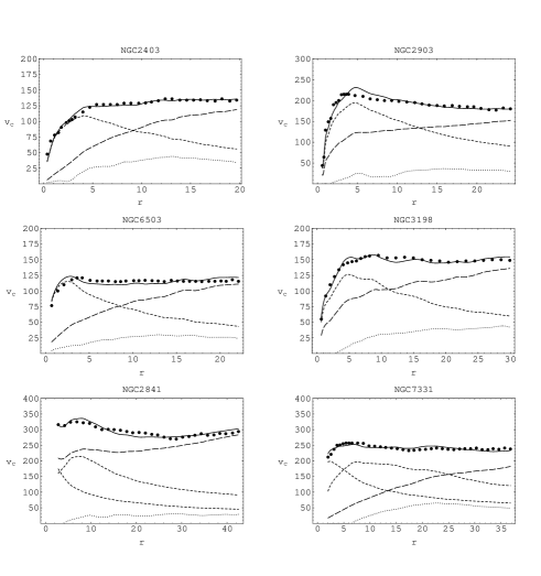
FIG. 4.: Curves of $v_{C}$ (km/s) vs $r$ (kpc) for the observational data (dots) and the fits from equation (60) (solid). Also shown are the individual contributions from luminous matter (short dashed), the scalar field (long dashed) and gas (dotted). In the case of NGC 2841 and NGC 7331, the lower short dashed curve represents the contribution from the bulge of these galaxies.

$$v_{C}^{2}(r)=\frac{GM_{L}(r)}{r}(1+f_{0}(r^{2}+b^{2}))+v_{gas}^{2}.$$ (60)

The main results are shown in Fig. 4 and in Table 1 (see also [44]), in which there are shown the observational RC (for simplicity we have omitted the error bars) as well as the best fit parameters for the generated curves using equation (60). Shown are also the individual contributions from luminous matter, gas and the scalar field. It can be noted that the agreement is quite good (within 5% in all cases), which could have been expected since there are three parameters to be adjusted.

The remaining two parameters, $f_{0}$ and $b$, serve only to determine completely the metric, and they do not have a direct physical interpretation other than as part of the scalar field energy density.

A A particular case: spherical symmetry

Analogously, assuming that the halo has spherically symmetry (a particular case of the previous symmetry) the space-time with the flat curve condition, it is easy to find the (see [43, 45]) becomes in general

$$ds^{2}=-B_{0}r^{m}dt^{2}+A(r)dr^{2}+r^{2}d\theta^{2}+r^{2}\sin^{2}\theta d\varphi^{2}$$ (61)

with $m=2(v^{\varphi})^{2}$ preserving the meaning of $v^{\varphi}$. This result is not surprising. Remember that the Newtonian potential $\psi_{N}$ is defined as $g_{00}=-\exp(2\psi_{N})=-1-2\psi_{N}-\cdots$. On the other side, the observed rotational curve profile in the dark matter dominated region is such that the rotational velocity $v^{\varphi}$ of the stars is constant, the force is then given by $F=-(v^{\varphi})^{2}/r$, which respective Newtonian potential is $\psi=(v^{\varphi})^{2}\ln(r)$. If we now read the Newtonian potential from the metric (61), we just obtain the same result. Metric (61) is then the metric of the general relativistic version of a matter distribution, which test particles move in constant rotational curves. Function $A(r)$ will be determined by the kind of substance we are supposing the dark matter is made of.

However, the case we are putting forward in this moments corresponds to the case of a stress-energy tensor corresponding to a scalar field, for which, when assumed the equivalent potential found for the axial case (44)

$$V(\Phi)=-\frac{m}{\kappa_{0}(2-m)}\exp\left[-2\sqrt{\frac{\kappa_{0}}{m}}(\Phi-\Phi_{0})\right]$$ (62)

the interesting line element reads:

$$ds^{2}=-B_{0}r^{m}dt^{2}+dr^{2}+\frac{4}{4-m^{2}}r^{2}\left[d\theta^{2}+\sin^{2}\theta d\varphi^{2}\right]$$ (63)

for which the two dimensional hypersurface area is $4\pi r^{2}\times 4/(4-m^{2})=4\pi r^{2}/(1-(v^{\varphi})^{4})$. Observe that if the rotational velocity of the test particles were the speed of light $v^{\varphi}\rightarrow 1$, this area would grow very fast. Nevertheless, for a typical galaxy, the rotational velocities are $v^{\varphi}\sim 10^{-3}$ ($300km/s$), in this case the rate of the difference of this hypersurface area and a flat one is $(v^{\varphi})^{4}/(1-(v^{\varphi})^{4})\sim 10^{-12}$, which is too small to be measured, but sufficient to give the right behavior of the motion of stars in a galaxy. The effective density depends on the velocities of the stars in the galaxy, $\rho=(v^{\varphi})^{4}/(1-(v^{\varphi})^{4})\times 1/(\kappa_{0}r^{2})$ which for the typical velocities in a galaxy is $\rho\sim 10^{-12}\times 1/(\kappa_{0}r^{2})$, while the effective radial pressure is $|P|=(v^{\varphi})^{2}((v^{\varphi})^{2}+2)/(1-(v^{\varphi})^{2})\times 1/(\kappa_{0}r^{2})\sim 10^{-6}\times 1/(\kappa_{0}r^{2})$, $i.e.$, six orders of magnitude greater than the scalar field density. This is the reason why it is not possible to understand a galaxy with Newtonian dynamics. Newton theory is the limit of the Einstein theory for weak fields, small velocities but also for small pressures (in comparison with densities). A galaxy fulfills the first two conditions, but it has pressures six orders of magnitude bigger than the dark matter density, which is the dominating density in a galaxy. This effective pressure is the responsible for the behavior of the flat rotation curves in the dark matter dominated part of the galaxies.

Metric (63) is not asymptotically flat, it could not be so. An asymptotically flat metric behaves necessarily like a Newtonian potential provoking that the velocity profile somewhere decays, which is not the observed case in galaxies. Nevertheless, the energy density in the halo of the galaxy decays as

$$\rho\sim\frac{10^{-12}}{\kappa_{0}r^{2}}=\frac{10^{-12}H_{0}^{-2}}{3r^{2}}\rho_{crit}$$ (64)

where $H_{0}^{-1}=\sqrt{3}/h\ 10^{6}$ kpc is the Hubble parameter and $\rho_{crit}$ is the critical density of the Universe. This means that after a relative small distance $r_{crit}\sim\sqrt{3/h^{2}}\approx 3$ kpc the effective density of the halo is similar as the critical density of the Universe. One expects, of course, that the matter density around a galaxy is smaller than the critical density, say $\rho_{around}\sim 0.0002\rho_{crit}$, then $r_{crit}\approx 100$ kpc. Observe also that metric (63) has an almost flat three dimensional space-like hypersurface. The difference between a flat three dimensional hypersurface area and the three dimensional hypersurface area of metric (63) is $\sim 10^{-12}$ , this is the reason why the space-time of a galaxies seems to be so flat.

V The Galaxy Center

The study of the center of the galaxy is much more complicated because we do not have any direct observation of it. If we follow the hypothesis of the scalar dark matter, we cannot expect that the center of a galaxy is made of  “ordinary matter” , we expect that it contains baryons, self-interacting scalar fields, etc. There their states must in extreme conditions. At the other hand, we think that the center of the galaxy is not static at all. Observations suggest, for instance, an active nuclei. A regular solution that explains with a great accuracy the galactic nucleus is the assumption that there lies a boson star [46], which on the other hand would be an excellent source for the scalar dark matter [47]. It is possible to consider also the galactic nucleus as the current stage of an evolving collapse, providing a boson star in the galactic center made of a complex scalar field or a regular structure made of a time dependent real scalar field (oscillaton), both being stable systems [4, 5].

The energy conditions are no longer valid in nature, as it is shown by cosmological observations on the dark energy. Why should the energy conditions be valid in a so extreme state of matter like it is assumed to exist in the center of galaxies? If dark matter is of scalar nature, why should it fulfill the energy conditions in such extreme situation? In any case, the center of the galaxy still remains as a place for speculations.

VI Conclusions

We have developed most of the interesting features of a $95\%$ scalar-nature cosmological model. The interesting implications of such a model are direct consequences of the scalar potentials (1,5).

The most interesting features appear in the scalar dark matter model. As we have shown in this work, the solutions found alleviate the fine tuning problem for dark matter. Once the scalar field $\Phi$ atarts to oscillate around the minimum of its potential (5), we can recover the evolution of a standard cold dark matter model because the dark matter density contrast is also recovered in the required amount. Also, we find a Jeans lenght for this model. This provokes the suppression in the power spectrum for small scales, that could explain the smooth core density of galaxies and the dearth of dwarf galaxies. Up to this point, the model has only one free parameter, $\lambda$. However, if we suppose that the scale of suppression is $k=4.5h\,$ Mpc, then $\lambda\approx 20.3$, and then all parameters are completely fixed. From this, we found that $V_{0}\simeq(36.5\,{\rm eV})^{4}$ and the mass of the ultra-light scalar particle is $m_{\Phi}\simeq 1.1\times 10^{-23}\,{\rm eV}$. Considering that potential  (5) is renormalizable, we calculated the scattering cross section $\sigma_{2\rightarrow 2}$. From this, we find that the renormalization scale $\Lambda$ is of order of the Planck mass if we take the value required for self-interacting dark matter, as our model is also self-interacting.

The hypothesis of the scalar dark matter is well justified at galactic level (see also [45]) and at the cosmological level too [14]. But at this moment it is only that, a hypothesis which is worth to be investigated.

Summarizing, a model for the Universe where the dark matter and energy are of scalar nature can be realistic and could explain most of the observed structures and features of the Universe.

VII Acknowledgements

We would like to thank Vladimir Avila-Reese, Michael Reisenberger, Ulises Nucamendi and Hugo Villegas Brena for helpful discussions. L.A.U. would like to thank Rodrigo Pelayo and Juan Carlos Arteaga Velázquez for many helpful insight. F. S. G. wants to thank the criticism provided by Paolo Salucci related to the galactic phenomenology and the ICTP for its kind hospitality during the begining of this discussion. We also want to express our acknowledgment to the relativity group in Jena for its kind hospitality. This work is partly supported by CONACyT México under grant 34407-E,  and by grant 119259 (L.A.U.), DGAPA-UNAM IN121298 (D.N.) and by a cooperations grant DFG-CONACyT.

TABLE I.: Best-fit parameters

Galaxy	(M/L)disk	(M/L)bulge	b	f0
			(kpc)	(kpc-1)
NGC 2403	1.75	–	1.63	0.0116
	0.04	–	0.003	$5.7\times 10^{-4}$
NGC 2903	2.98	–	8.33	0.0043
	0.12	–	0.03	$4.0\times 10^{-4}$
NGC 6503	2.12	–	1.79	0.013
	0.09	–	0.01	$8.7\times 10^{-4}$
NGC 3198	2.69	–	7.83	0.0054
	0.08	–	0.02	$3.0\times 10^{-4}$
NGC 2841	5.39	3.25	13.85	0.0039
	0.34	0.36	0.16	$2.5\times 10^{-4}$
NGC 7331	5.06	1.11	0.845	0.0013
	0.23	0.06	0.002	$8.9\times 10^{-5}$

REFERENCES

- [1] D. N. Schramm, In “Nuclear and Particle Astrophysics”, ed. J. G. Hirsch and D. Page, Cambridge Contemporary Astrophysics, (1998). Shi, X., Schramm, D. N. and Dearborn, D., Phys. Rev. D 50, (1995) 2414.
- [2] H. Dehnen and B. Rose, Astrophys. Sp Sci. 207 (1993) 133-144.
- [3] H. Dehnen, B. Rose and K. Amer, Astrophys. Sp Sci. 234 (1995) 69-83.
- [4] E. Seidel and W. Suen, Phys. Rev. Lett. 72 (1994) 2516.
- [5] J. Balakrishna, E. Seidel and W. Suen, Phys. Rev. D (1999) 104004.
- [6] P. J. E. Peebles, “Principles of Physical Cosmology”, Princeton University Press, (1993).
- [7] M. Persic, P. Salucci and F. Stel, MNRAS 281 (1996) 27-47.
- [8] K. G. Begeman, A. H. Broeils and R. H. Sanders, MNRAS 249 (1991) 523.
- [9] S. Perlmutter et al. Astrophys. J. 517 (1999) 565. A. G. Riess et al., AJ 116 (1998) 1009.
- [10] N. A. Bahcall, J. P. Ostriker, S. Perlmutter and P. J. Steinhardt, Science 284 1481. V. Sahni, A. Starobinsky, Int. J. Mod. Phys. D 9 (2000) 373.
- [11] V. Sahni and L. Wang, Phys. Rev. D 62 (2000) 103517.
- [12] F. S. Guzmán and T. Matos, Class. Quantum Grav. 17 (2000) L9-L16. T. Matos and F. S. Guzmán, Ann. Phys. (Leipzig) 9 (2000) SI 133-136. T. Matos, F. S. Guzmán and D. Núñez, Phys. Rev. D 62 (2000) 061301.
- [13] T. Matos, F. S. Guzmán and L. A. Ureña-López, Class. Quantum Grav. 17 (2000) 1707.
- [14] T. Matos and L. A. Ureña-López, Class. Quantum Grav. 17 (2000) L71.
- [15] L. A. Ureña-López and T. Matos, Phys. Rev. D 62 (2000) 081302.
- [16] P. de Bernardis et al., Nature (London) 404 (2000) 955-959. S. Hanany et al. , preprint astro-ph/0005123.
- [17] L. P. Chimento, A. S. Jakubi, Int. J. Mod. Phys. D 5(1996) 71.
- [18] Pedro G. Ferreira and Michael Joyce, Phys. Rev. D 58 (1998) 023503.
- [19] M. S. Turner, Phys. Rev. D 28 (1983) 1243. L.H. Ford, Phys. Rev. D 35 (1987) 2955.
- [20] T. Matos and L. A. Ureña-López, Phys. Rev. D63, (2001), 063506. Preprint astro-ph/0006024.
- [21] R. R. Caldwell, R. Dave and P. J. Steinhardt, Phys. Rev. Lett. 80 (1998) 1582. I. Zlatev, L. Wang and P. J. Steinhardt, Phys. Rev. Lett. 82 (1999) 896. P.J. Steinhardt, L. Wang and I. Zlatev, Phis. Rev. D 59 (1999) 123504.
- [22] C.-P. Ma and E. Berthshinger, Astrophys. J. 455 (1995) 7.
- [23] C.-P. Ma et al, Astrophys. J. 521 (1999) L1-L4.
- [24] P. Brax, J. Martin and A. Riazuelo, Phys. Rev. D 62 (2000) 103505.
- [25] U. Seljak and M. Zaldarriaga, Astrophys. J. 469 (1996) 437.
- [26] Marc Kamionkowski and Andrew R. Liddle, Phys. Rev. Lett. 84 (2000) 4525.
- [27] W. Hu, R. Barkana and A. Gruzinov, Phys. Rev. Lett. 85, (2000) 1158.
- [28] B. D. Wandelt, R. Dave, G. R. Farrar, P. C. McGuire, D. N. Spergel and P.J. Steinhardt, astro-ph/0006344.
- [29] C. Firmani, E. D’Onghia, G. Chincarini, X. Hernández and V. Ávila-Reese, preprint astro-ph/0005001. V. Ávila-Reese, C. Firmani, E. D’Onghia and X. Hernández, astro-ph/0007120.
- [30] P. Colín, V. Ávila-Reese and O. Valenzuela, astro-ph/0004115.
- [31] D. N. Spergel and P. J. Steinhardt, Phys. Rev. Lett. 84 (2000) 3760.
- [32] K. Halpern and K. Huang, Phys. Rev. Lett. 74 (1995) 3526. K. Halpern and K. Huang, Phys. Rev. D 53 (1996) 3252
- [33] V. Branchina, hep-ph/0002013.
- [34] T. Matos and L. A. Ureña-López, astro-ph/0010226.
- [35] K. Halpern, Phys. Rev. D 57 (1998) 6337.
- [36] M.C. Bento, O. Bertolami and R. Rosenfeld, Phys. Rev. D 62 (2000) 041302.
- [37] E. Gessner, Astrophys. Sp Sci. 196 (1992) 29-43.
- [38] F. S. Guzmán, T. Matos and H. Villegas-Brena, Astron. Nachr. 320 (1999) 3, 97.
- [39] E. Schmutzer, “Kosmoligie ohne Urknall auf der Basis der Projektiven Einheitlichen Feldtheorie”. Forschungsbeiträge der Naturwissenschaftlichen Klasse, München 1998.
- [40] E. Schmutzer, Astron. Nachr. 320 (1999) 1.
- [41] Vera C. Rubin, W. Kent Ford and Norbert Thonnard, AJ 238 (1980) 471-487.
- [42] D. Kramer, H. Stephani, E. Herlt and M. MacCallum, “Exact Solutions of Einstein’s Field Equations”. Ed. by E. Schmutzer, Cambridge University Press, (1980).
- [43] T. Matos, D. Nuñez, F. S. Guzmán and E. Ramírez, to be published. Preprint astro-ph/0005528.
- [44] T. Matos and F. S. Guzmán, Rev. Mex. A & A, accepted. Preprint astro-ph/9811143.
- [45] T. Matos, F. S. Guzmán and D. Núñez, Phys. Rev. D 62 (2000) 061301.
- [46] D. F. Torres, S. Capozziello and G. Lambiase, Phys. Rev. D 62 (2000) 104012.
- [47] T. Matos, L. A. Ureña-López and F. S. Guzmán, to be published.