Acceleration and collimation of relativistic plasmas ejected by fast rotators

Abstract

A stationary self-consistent outflow of a magnetised relativistic plasma from a rotating object with an initially monopole-like magnetic field is investigated in the ideal MHD approximation under the condition $\sigma/U_{0}^{2}>1$, where $\sigma$ is the ratio of the Poynting flux over the mass energy flux at the equator and the surface of the star, with $U_{0}=\gamma_{0}v_{0}/c$ and $\gamma_{0}$ the initial four-velocity and Lorentz factor of the plasma. The mechanism of the magnetocentrifugal acceleration and self-collimation of the relativistic plasma is investigated. A jet-like relativistic flow along the axis of rotation is found in the steady-state solution under the condition $\sigma/U_{0}^{2}>1$ with properties predicted analytically. The amount of the collimated matter in the jet is rather small in comparison to the total mass flux in the wind. An explanation for the weak self-collimation of relativistic winds is given.

1 Introduction

Radio pulsars (Michel michel91 (1991)), superluminal galactic objects (Mirabel & Rodriguez mirabel94 (1994), mirabel99 (1998)) and AGNs (Begelman, Blandford & Rees blandford (1984), Pelletier et al. pelletier (1996)) are observed to be associated with relativistic outflows. AGNs and superluminal galactic objects produce jets, while radio pulsars demonstrate a surprisingly high efficiency of transforming the pulsar rotational energy into kinetic energy of the relativistic wind (Kennel & Coroniti kennel (1984)). Hence, the problem of acceleration and collimation of relativistic plasmas is among the most important in the physics of relativistic outflows.

Nevertheless, radio pulsars, AGNs and superluminal galactic objects are objects of rather different nature and scales. It may well be that the mechanisms of acceleration of the outflows in these sources are not the same. However, there seems to exist a mechanism which operates very well for all these objects, namely, the so-called magnetocentrifugal acceleration where the acceleration of the plasma outflow occurs in the magnetic field of the rotating object. Such conditions are realized in the magnetospheres of radio pulsars, in the winds from accretion disks (Blandford & Payne bp (1982)) and apparently in superluminal galactic objects (Mirabel & Rodriguez mirabel99 (1998)). However, it has not been investigated whether the magnetocentrifugal mechanism could provide the acceleration of the relativistic plasma in these objects to the observed bulk motion velocities.

The analysis of problem of the relativistic plasma acceleration and collimation in a rotating magnetosphere started with Michel (michel (1969)), where it was shown that the magnetocentrifugal acceleration of the plasma is not effective for a prescribed monopole-like magnetic field. Subsequently, the relativistic plasma outflow has been investigated in several other studies and for different astrophysical conditions (Okamoto okamoto78 (1978), Ardavan ardavan (1979), Beskin et al. bgi (1983), Camenzind max86 (1986)). In particular, the ultrarelativistic plasma outflow from an accretion disk was investigated numerically in Camenzind (max87 (1987)) while the structure of electromagnetically driven relativistic jets was discussed in Li (li93 (1993)) under the assumption of jet confinement by an ambient medium. Collimation of stellar magnetospheres to jets in the force-free approximation was studied in Sulkanen & Lovelace (ml (1990)) and Fendt et al. (fendt95 (1995)). Later, Fendt & Camenzind (fendt96 (1996)) investigated the plasma dynamics in the MHD approximation in magnetic configurations obtained via the force-free approximation. A class of self-similar solutions of the relativistic plasma outflow has been obtained in Contopoulos (ianos94 (1994)). It was found that the efficiency of the plasma acceleration can be higher than in Michel’s solution due to the effect of the magnetic collimation of the wind to the axis of rotation (Begelman & Li (li (1994)), Fendt & Camenzind fendt96 (1996), Takahashi & Shibata (ts (1998))). Thus, the problem of the relativistic plasma acceleration in a rotating magnetic field appeared to be closely connected to the problem of plasma collimation.

Strong evidence has been accumulated for a correlation between collimated astrophysical outflows (jets) and accretion disks. Direct evidence for a disk-jet connection has been demonstrated by HST observations of the Herbig-Haro object HH30 (Burrows et al. burrows (1996)), although on the theoretical front this connection was discussed earlier (Camenzind max90 (1990), Ferreira & Pelletier ferreira (1993), Falke & Biermann falke (1995)). A disk-jet connection is also supported by observations of the active galaxy M87 (Ford et al. ford (1994)) and superluminal galactic objects (Mirabel & Rodriguez mirabel98 (1998)). These observations seem to lead to the conclusion that jets require the existence of accretion disks for their formation (e.g. Livio livio (1999)) and therefore accretion disks should be a necessary element of the collimation mechanism. However, we have by now reliable evidence that there is at least one source producing jets without the presence of an accretion disk. Namely, recent observations of the Crab Nebula by the Chandra observatory leave no doubts that the Crab pulsar indeed produces jets (Weiskopff et al. crab (2000)). Therefore, it would be important to understand the mechanism of plasma collimation in all known jet sources, including the Crab pulsar.

Such a mechanism is provided by magnetic collimation of outflows from accretion disks and it was first suggested by Lovelace (lovelace (1976)), Blandford (blandford76 (1976)) and Bisnovatyi-Kogan & Ruzmaikin (bkgr (1976)). Subsequently, it was shown from an analysis of the full set of the MHD equations for nonrelativistic (Heayvaerts & Norman heyvaerts (1989)) and relativistic outflows (Chiueh et al. chiueh (1991), Bogovalov bog95 (1995)) that collimation is a rather general property of magnetised winds from a rotating object. A magnetised fast-mode supersonic wind inevitably will be partially cylindrically collimated along the axis of rotation at distances large compared to all characteristic dimensions of the source, such as the size of the accretion disk, provided that: the flow is non-dissipative, the magnetised central object is rotating, the total magnetic flux of one polarity reaching infinity (open field lines) is finite, the polytropic index of the plasma exceeds unity and the pressure of ambient matter is low enough not to be able to terminate the wind before the formation of the jet. This result is independent of the specific properties of the central source. Collimation occurs spontaneously due to the internal Lorentz force arising in the magnetised plasma which is ejected from the rotating source and therefore can be regarded as a process of self-collimation (hereafter SC process). Note that the assumption of a polytropic gas with a constant polytropic index $\gamma$ does not seem really restrictive, since several exact MHD solutions for collimated outflows have been constructed for the case of a variable index $\gamma$, Sauty & Tsinganos (1994), Vlahakis & Tsinganos (1998).

Although the SC process has been questioned (e.g., Okamoto okamoto99 (1999)), a numerical investigation of this process and the characteristics of jets produced via this mechanism in the cold (Bogovalov & Tsinganos bogts (1999)) or hot (Tsinganos & Bogovalov tsbog (2000), Sauty et al (1999)) nonrelativistic winds leave no doubt that this mechanism works. This mechanism provides the formation of cylindrically collimated outflows at a large distance from the central source while collimation is accompanied by essentially more efficient acceleration of the plasma at the equatorial region as compared with the original study of Michel (michel (1969)). Evidence for the focusing of MHD outflows from accretion disks to the axis of rotation at distances of the order of the dimension of accretion disks has been obtained in other studies as well, such as in Ouyed & Pudritz (op (1997)), Ustyugova et.al. (ustyug (1999)) and Krasnopolskii et. al. (krasno (1999)).

In the analysis of Bogovalov & Tsinganos (1999), the relaxation method was used to obtain the solution of the steady state outflow problem, i.e., the time-dependent problem was solved in order to get a steady-state solution. This method was first employed by Washimi & Shibata (shibata (1993)) for outflows from stellar objects. Later this method was applied in Bogovalov (1996) for the investigation of the SC process in an initially monopole-like magnetic field. It seems that this numerical method allows us to solve accurately all problems connected with the critical surfaces (Bogovalov 1997b , Tsinganos et al. tsincr (1996)).

In our previous study (Bogovalov 1997a ), the relaxation method has been applied to the investigation of the relativistic plasma outflow and it was found that the relativistic plasma is very weakly collimated and accelerated even if the Poynting flux dominates the matter energy flux at the equator. However, an analytical study performed in this work has shown that an efficient SC of the relativistic plasma is still possible for very fast rotation of the central source. Recently it has been argued that a relativistic plasma is poorly accelerated even under this condition (Beskin et al. beskin98 (1998)). However, the SC process was totally neglected in this work. Therefore, the question concerning the efficiency of the acceleration and SC of the relativistic winds from fast rotators remains open.

2 Basic assumptions

Outflows of magnetised plasmas are described by the system of the familiar nonlinear MHD equations. It is not surprising that this system has many solutions corresponding to different physical conditions. Then, a reasonable choice of the appropriate approximation and a sound model is crucially important to arrive at some physically meaningful solution.

To formulate the basic demands of the model let us consider the general properties of winds and jets. According to observations, the length of the jets greatly exceeds all characteristic scales of the central source. Therefore, for an investigation of the SC process and the characteristics of the jets, the theory should allow us to obtain the solution on scales greatly exceeding all sizes of the central source.

Observations of winds and jets from several classes of astrophysical objects such as our Sun (Parker parker (1963)), or, YSO’s (Burrows et al. burrows (1996)), pulsars (Kennel & Coroniti kennel (1984)) and AGNs (Ferrari et al. ferrari (1996)) show that they are super-magnetosonic at relatively large distances from the source. At the same time all winds must be subsonic near the central source where the basic parameters of the outflows are controlled. Therefore, the theory must describe flows of mixed type, containing the small scale regions of a subsonic flow and the large scale regions of the super magnetosonic flow. The scales of these regions may differ by several orders of magnitude. These properties of the outflows dictate the choice of the approximations and mathematical models.

2.1 Approximations

The force-free approximation has been widely used for the analysis of axisymmetric relativistic outflows (Scharlemann & Wagoner sw (1973), Mestel & Wang mw (1979), Beskin et al. bgi (1983), Lyubarskii lyubarskii (1990), Fendt et al. fendt95 (1995)). For simplification reasons, the axisymmetric stellar magnetosphere can be assumed initially to have a dipolar magnetic field (Contopoulos et al.kazanas (1999)). However, this approximation is not appropriate for the investigation of the SC process for several reasons. For example, it describes only subsonic flows of plasma since the force-free transfield (Grad-Shafranov) equation is elliptic everywhere (Fendt et al. fendt95 (1995)). Therefore, this approximation cannot be used for the investigation of plasma outflow in the supersonic regions. Moreover, the collimating and accelerating forces are equal to zero in this approximation. For these reasons, the force-free approximation gives ambiguous results. For example, the structure of the flow of the relativistic plasma at large distances from the source obtained in Sulkanen & Lovelace ml (1990) and in Fendt et al. fendt95 (1995) differs from the structure obtained in Contopoulos et al. (kazanas (1999)). Although Sulkanen & Lovelace (ml (1990)) and Contopoulos et al. (kazanas (1999)) used similar models, Contopoulos et al. (kazanas (1999)) obtained a radially outflowing plasma while Sulkanen & Lovelace (ml (1990)) obtained collimated jets. Jets were obtained as well in Fendt et al. (fendt95 (1995)). Actually all these works are mathematically correct. The difference between them is only in the boundary conditions at infinity or at the outer boundary of the integration domain. These works clearly demonstrate that the flow of plasma at large distances from the source in the force-free approximation basically depends on the boundary conditions at infinity. But there is no such dependence in real supersonic flows. This is the most important qualitative difference between the subsonic and super fast magnetosonic flows.

In the steady state subsonic flow the MHD signals propagate down and upstream of the flow. That is why the plasma flow is defined by the forces affecting the plasma at a given point, upstream and down stream of the flow. This is not the case in the super fast magnetosonic flow. No MHD signals can propagate upstream of the supersonic flow. The supersonic flow is defined only by the forces which affect the plasma upstream and at the given point and does not depend on the forces which affect the plasma downstream of the flow. For this reason the supersonic flow does not depend on the boundary conditions located downstream of the flow (actually the situation is more complicated; the flow should cross the fast mode critical surface, Bogovalov 1997b ). The simplest approximation which allows us to describe the mixed type outflows is the ideal MHD approximation. This approximation is used in this paper.

2.2 Model

However, even the use of the MHD approximation does not always allow us to investigate the SC process in the supersonic region. There is a wide class of self-similar solutions for the nonrelativistic (Blandford & Payne bp (1982), Vlahakis & Tsinganos tv (1999) e.g.) and relativistic plasma (Contopoulos ianos94 (1994)). All these solutions terminate not so far from the source. Independent of why this termination happens, the self-similar solutions cannot be used for the verification of the predictions of the SC theory since the central source has infinitely large size with infinite magnetic flux in the upper hemisphere. At any distance from the source, the dimension of the source exceeds the distance to the source. However, we are interested in the opposite case, when the distance is large compared with the dimension of the central source. Therefore, we demand that the appropriate model should have finite geometrical dimensions, finite magnetic flux of the open field lines of every polarity and initially uncollimated plasma outflow. The last condition is important for us since our objective is to study the process which transforms the initially uncollimated outflow into the outflow containing the jet. The word “initially” means that if one of the conditions for the SC process is not fulfilled (for example if the central source is not rotating or the magnetic field is absent) the wind expands radially at large distances from the source. Actually, a lot of models satisfy all these conditions.

The SC is a general property of magnetised winds from rotating sources. It must take place in a wind from any source provided that the conditions specified by Heayvaerts & Norman (heyvaerts (1989)), Chiueh et al. (chiueh (1991)) and Bogovalov (bog95 (1995)) are fulfilled. Therefore “convenience” and “simplicity” become reasonable arguments for the choice of the model for the investigation of this process. The model of a star with a wind in an initially monopole-like (below m-l) magnetic field firstly proposed by Sakurai (sakurai (1985)) is the most simple and convenient. This model allows us to avoid the mathematically complicated problem connected with the coexistence of open and closed field lines near the source which actually has no direct relation to the SC process and usually is considered particular (Keppens & Goedbloed keppens (1999)).

The model with the initially monopole-like magnetic field describes more a wider class of outflows, including the time-dependent outflows from oblique rotators (Bogovalov bog99 (1999)) and outflows from objects with arbitrary distribution of the polarity of the magnetic field at the base (Tsinganos & Bogovalov tsbog (2000)).

In this paper we consider the outflow of an initially cold relativistic plasma and neglect only gravitation since we are interested in the effect of the electromagnetic forces only on the plasma.

3 Basic equations and methods of solution.

The plasma outflow from astrophysical objects consists of two zones where the properties of the flow differ qualitatively. The nearest zone is located near the surface of the central source and includes all the critical surfaces of the steady state flow (Bogovalov 1997b ). The outer boundary of the nearest zone can be located rather arbitrary but always downstream of the fast mode critical surface. The flow of the plasma in the nearest zone is of the mixed type. It is subsonic near the source and is super fast magnetosonic at the outer boundary. The far zone is located downstream of the nearest zone. The plasma flow in the far zone is super fast magnetosonic. Different methods should be applied for the solution of the problem in each of these zones.

The solution of the problem of the steady state plasma outflow can be divided in two steps (Bogovalov & Tsinganos bogts (1999)). In the first step, the problem is solved in the nearest zone by the relaxation method and in the second, the steady state solution in the far zone is obtained by solving directly the transfield equation as a Cauchy problem. The solution in the nearest zone is used to specify the initial values for the flow in the far zone.

3.1 Solution in the nearest zone.

The system of equations defining the dynamics of the relativistic plasma in the ideal MHD approximation is as follows,

$$\rho c({\bf\dot{U}}+({\bf v}\cdot{\bf\nabla}){\bf U})=q{\bf E}+{1\over c}{\bf j\times B},$$ (1)

$${\bf E}+{1\over c}{\bf v\times B}=0,$$ (2)

$${\bf\nabla\times B}={4\pi\over c}{\bf j}+{1\over c}\bf\dot{E},$$ (3)

$${1\over c}\bf\dot{B}=-{\bf\nabla\times E},$$ (4)

$$\dot{\rho}+({\bf\nabla\cdot v}\rho)=0.$$ (5)

Here $q=({\bf\nabla\cdot\bf E})/4\pi$ is the induced electric charge density, $\bf j$ is the electric current density, $\bf E$ is the electric field, ${\bf U=v}\gamma/c$ is the spatial component of the plasma four-velocity and $\rho$ is the mass density of the plasma.

The problem was solved in the cylindrical system of coordinates. Some details of the solution method are given in appendix A. The numerical simulation was performed only in the quarter of the total box of simulation due to the symmetry of the flow in relation to the equatorial plane and the axis of rotation. The boundaries of the nearest zone include the surface of the star, the axis of rotation, the equator and the outer boundaries, which are a cylinder (right hand side of the box) and a plane perpendicular the axis of rotation at some distance from the source (upper side of the box). The outer boundaries are located in the supersonic domain of the flow beyond the fast mode critical surface. This guarantees the independence of the solution in the nearest zone of the position and conditions of the outer boundaries.

The number of independent boundary conditions on the surface of the star is equal to the number of MHD waves leaving the surface to satisfy the causality in the flow (Bogovalov 1997b ). They are as follows:
1. A constant plasma density $\rho_{0}$.
2. A constant Lorentz-factor $\gamma_{0}$ of the plasma in the corotating frame system.
3. A constant normal component of the poloidal magnetic field $B_{0}$.
4. The continuity of the tangential component of the poloidal electric field.
5. A constant temperature of the plasma equal to zero.

The boundary conditions at the axis of rotation correspond to the axial symmetry of the flow. The boundary conditions at the equator follow from the symmetry of the flow in relation to the equatorial plane. This means that $\rho(z)=\rho(-z)$, $v_{r}(z)=v_{r}(-z)$, $v_{z}(z)=-v_{z}(-z)$, $B_{r}(z)=B_{r}(-z)$, $B_{z}(z)=-B_{z}(-z)$, $v_{\varphi}(z)=v_{\varphi}(-z)$ and $B_{\varphi}(z)=B_{\varphi}(-z)$.

At the outer boundaries only one side internal derivatives were used for calculation of the derivatives in the finite differences, since the solution does not depend on the conditions down the flow from these boundaries.

3.2 Solution in the far zone

The flow in the far zone is fast mode supersonic. The system of equations describing the steady state flow is hyperbolic. Therefore, a Cauchy problem can be formulated for this flow.

It is convenient to introduce the flux function $\psi$ as follows

$${\bf B}_{p}={{\bf\nabla}\psi\times\hat{\bf\varphi}\over r},$$ (6)

Where $B_{p}$ is the poloidal magnetic field of the axisymmetric outflow and $\hat{\bf\varphi}$ is the unit azimuthal vector.

The stationary MHD equations admit well known four integrals (Tsinganos tsin82 (1982)). They are:

($\alpha$)

The ratio of the poloidal magnetic and mass fluxes, $F(\psi)$

$$F(\psi)={B_{p}\over 4\pi\rho v_{p}c}\,.$$ (7)

($\beta$)

The total angular momentum per unit mass $L(\psi)$,

$$rU_{\varphi}-FrB_{\varphi}=L(\psi)\,.$$ (8)

($\gamma$)

The corotation frequency $\Omega(\psi)$ in the frozen-in condition

$$U_{\varphi}B_{p}-U_{p}B_{\varphi}=r\gamma B_{p}\Omega(\psi)/c\,.$$ (9)

($\delta$)

The total energy $W(\psi)$ per particle in the equation for total energy conservation,

$$\gamma-F(\psi)r\Omega(\psi)B_{\varphi}/c=W(\psi)\,.$$ (10)

This system of equations should be supplemented by a relativistic relationship between the components of the four-velocity

$$\gamma^{2}=1+U_{p}^{2}+U_{\varphi}^{2}.$$ (11)

Momentum balance across the poloidal field lines is expressed by the transfield equation. For analysing the behavior of the plasma at large distances, it is convenient to deal with this equation in an orthogonal curvilinear coordinate system ($\psi,\eta$) formed by the poloidal magnetic field lines and by the lines of the poloidal electric field. $\psi$ varies with the motion across the magnetic field lines, while $\eta$ varies with the motion along the magnetic field lines. A geometrical interval in these coordinates can be expressed as

$$(d{\bf r})^{2}=g^{2}_{\psi}d\psi^{2}+g^{2}_{\eta}d\eta^{2}+r^{2}d\varphi^{2},$$ (12)

where $g_{\psi},g_{\eta}$ are the corresponding line elements (components of the metric tensor).

According to Landau & Lifshitz (1975) the equation $T_{\psi;k}^{k}=0$, where $T^{ij}$ is the energy-momentum tensor and ”; k” denotes covariant differentiation, will have the following form in these coordinates,

$$\begin{array}[]{c}{\partial\over\partial\psi}\left[{B^{2}-E^{2}\over 8\pi}\right]-{1\over r}{\partial r\over\partial\psi}\left[U_{\varphi}v_{\varphi}c\rho-{B_{\varphi}^{2}-E^{2}\over 4\pi}\right]-\\ \\ {1\over g_{\eta}}{\partial g_{\eta}\over\partial\psi}\left[U_{p}v_{p}c\rho-{B_{p}^{2}-E^{2}\over 4\pi}\right]=0\end{array}$$ (13)

with the electric field $E={r\Omega\over c}B_{p}$.

The unknown variables here are $z(\eta,\psi)$ and $r(\eta,\psi)$. The metric coefficient $g_{\eta}$ can be obtained from the transfield equation (13),

$$g_{\eta}=\exp{(\int\limits_{0}^{\psi}G(\eta,\psi)d\psi)}\,,$$ (14)

where

$$G(\eta,\psi)={{\partial\over\partial\psi}\left[{B^{2}-E^{2}\over 8\pi}\right]-{1\over r}{\partial r\over\partial\psi}\left[U_{\varphi}v_{\varphi}c\rho-{B_{\varphi}^{2}-E^{2}\over 4\pi}\right]\over\left[U_{p}v_{p}c\rho-{B_{p}^{2}-E^{2}\over 4\pi}\right]}\,.$$ (15)

The lower limit of the integration in (14) is chosen to be 0 such that the coordinate $\eta$ is uniquely defined. In this way $\eta$ coincides with the coordinate $z$ where the surface of constant $\eta$ crosses the axis of rotation.

The metric coefficient $g_{\psi}$ can be obtained from definition (6) in terms of the magnitude of the poloidal magnetic field as follows

$$g_{\psi}={1\over rB_{p}}\,.$$ (16)

The orthogonality condition

$$r_{\eta}r_{\psi}+z_{\eta}z_{\psi}=0\,,$$ (17)

and the relationships

$$g^{2}_{\eta}=r_{\eta}^{2}+z_{\eta}^{2},\leavevmode\nobreak\ \leavevmode\nobreak\ \leavevmode\nobreak\ \leavevmode\nobreak\ g^{2}_{\psi}=r_{\psi}^{2}+z_{\psi}^{2}$$ (18)

give us that

$$r_{\eta}=-{z_{\psi}g_{\eta}\over g_{\psi}},\leavevmode\nobreak\ \leavevmode\nobreak\ \leavevmode\nobreak\ \leavevmode\nobreak\ z_{\eta}={r_{\psi}g_{\eta}\over g_{\psi}}\,,$$ (19)

with $g_{\eta}$ calculated by the expression (14). Here $r_{\eta}=\partial r/\partial\eta$, $z_{\eta}=\partial z/\partial\eta$, $r_{\psi}=\partial r/\partial\psi$, $z_{\psi}=\partial z/\partial\psi$. For the numerical solution of the system of equations (19) the two step Lax-Wendroff method on the lattice with a dimension equal to 1000 is used.

Equations (19) should be supplemented by appropriate boundary conditions and initial values on some initial surface of constant $\eta$ located in the nearest zone, but down the flow from all the critical surfaces. The form of the initial surface of constant $\eta$ was obtained numerically through integration of the following equations,

$${\partial r\over\partial\psi}={B_{z}\over rB_{p}^{2}},\leavevmode\nobreak\ \leavevmode\nobreak\ \leavevmode\nobreak\ \leavevmode\nobreak\ {\partial z\over\partial\psi}=-{B_{r}\over rB_{p}^{2}}\,.$$ (20)

The values $B_{z}$, $B_{r}$ and integrals $W(\psi),L(\psi),\Omega(\psi),F(\psi)$ were taken from the solution of the problem in the nearest zone.

Boundary conditions on the axis of rotation and the equatorial plane are the same as the conditions in the nearest zone. No conditions at infinity were specified.

4 Parameterisation of the solution

A stationary solution of the relativistic plasma flow from the star with an initially m-l magnetic field is defined by three dimensionless parameters (Bogovalov bog99 (1999)). One of them is the ratio of the radius of the star $R_{star}$ to the radius of the initial fast mode magnetosonic surface $R_{f}=\sqrt{(B_{0}R_{star})^{2}/4\pi\rho_{0}v_{0}cU_{0}}$, where $U_{0}=v_{0}\gamma_{0}/c$. The word ”initial” here refers to the radius of the fast mode surface when the star is not rotating. But this dependence can be neglected under the condition $R_{star}\ll R_{f}$ and $R_{star}\ll R_{l}$, where $R_{l}=c/\Omega$ is the radius of the light cylinder, and $\Omega$ is the angular velocity of the uniformly rotating star. Therefore, the solution crucially depends only on two dimensionless parameters which can be chosen rather arbitrary. It is convenient to choose one of them as follows

$$\sigma=({R_{f}\over R_{l}})^{2}={B_{0}^{2}\over 4\pi\rho_{0}\gamma_{0}v_{0}^{2}}({R_{star}\Omega\over c})^{2}.$$ (21)

$\sigma$ is the squared ratio of the initial radius of the fast mode surface to the light cylinder radius. According to (21) the radius of the light cylinder in units of $R_{f}$ is

$${R_{l}\over R_{f}}=\sqrt{1/\sigma}.$$ (22)

The parameter $\sigma$ is closely related to the so-called magnetisation parameter usually used in the physics of the relativistic winds from radio pulsars (Arons arons (1996)). The magnetisation parameter is the ratio of the Poynting flux density to the flux density of the mass energy (including rest mass energy). The parameter $\sigma$ used here is equal to the ratio of the Poynting flux to the mass energy flux at the equator of the rotator with the initially m-l magnetic field provided that $\sigma/U_{0}^{2}<<1$ (Bogovalov bog99 (1999)). In our previous work (Bogovalov 1997a ), we used another definition of the $\sigma$ parameter introduced initially by Michel (michel (1969)). This parameter is denoted by $\sigma_{M}$. There is a simple relationship between them $\sigma_{M}=\sigma U_{0}$. It follows from this relationship that $\sigma_{M}$ is equal to the Poynting flux density per particle on the equator provided that $\sigma/U_{0}^{2}<<1$.

It is convenient to take the second parameter as follows

$$\alpha={R_{f}\over R_{l}U_{0}}={\sqrt{\sigma}\over U_{0}}.$$ (23)

The physical sense of this parameter becomes clear if we pay attention to the fact that in the model of Michel (michel (1969)) the terminating four-velocity of the plasma on the equator is $U_{\infty}=(\sigma_{M}^{1/3})$ and $\alpha$ can be presented as follows

$$\alpha=(U_{\infty}/U_{0})^{3/2}.$$ (24)

According to Eq. (24), the parameter $\alpha$ shows how effectively the magnetic forces arising in the rotating magnetic field accelerate the plasma. If $\alpha<1$ acceleration is not important compared to the initial velocity of the plasma. It is natural to call the rotators with $\alpha<1$ as slow rotators. Correspondingly, the rotators with $\alpha\geq 1$ should be fast rotators which could in principle (but not necessarily) accelerate the plasma. The parameter $\alpha$ introduced here is the relativistic generalization of the $\alpha$ parameter introduced earlier by Bogovalov & Tsinganos (bogts (1999)) for the nonrelativistic plasma. Numerical simulations of the nonrelativistic plasma outflow show that this parameter indeed divides rotators into two groups with different efficiency of acceleration and collimation of the plasma. Below we will see that this division remains valid also in the relativistic limit.

Representation of the solution in the parameters $\alpha$, $\sigma$ is convenient since the steady state outflow in the initially m-l magnetic field has a simple analytical solution in the limit $\alpha\rightarrow 0$ independent of the value of $\sigma$ (Bogovalov 1997a ) and the transition to the nonrelativistic limit corresponds simply to the limit $\sigma\rightarrow 0$ and $v_{0}/c\ll 1$.

For comparison with observation, Eq. (21) should be expressed in variables general for the m-l model and real astrophysical objects. An astrophysical object can be considered as equivalent to the object with the m-l magnetic field if they both produce winds with the same magnetic flux, the same mass flux, the same initial Lorentz factor and finally both rotate with the same angular velocity. The magnetisation parameter in these variables takes the form

$$\sigma={\psi_{t}^{2}\over(2\pi)^{2}m\dot{N}\gamma_{0}v_{0}}({\Omega\over c})^{2},$$ (25)

where $\psi_{t}$ is the open field lines flux of one polarity in the wind, $\dot{N}$ is the rate of ejection of particles with mass $m$. For radio pulsars, $\psi_{t}=\pi B_{0}R_{p}^{2}$ where $R_{p}=R_{star}\sqrt{R_{star}\Omega/c}$ is the radius of the polar cap on the surface of the pulsar ( Ruderman & Sutherland rs (1975)).

The position of the radio pulsars in the parameter space $\alpha$, $\sigma$ was discussed in detail by Bogovalov (bog99 (1999)). All radio pulsars eject Poynting-dominated winds ($\sigma>1$) but basically all of them are slow rotators ($\alpha<1$). One of the youngest and fastest rotating pulsars with a strong magnetic field on the surface is the pulsar in the Crab Nebula. This pulsar rotates with $\Omega\approx 200$ and ejects $e^{\pm}$ pairs with the rate $\dot{N}\approx 4\cdot 10^{38}$ per second and average $\gamma_{0}\sim 200$ ( Daugherty & Harding dh (1982)). At $B_{0}\approx 4\cdot 10^{12}$ G the magnetisation parameter of the wind $\sigma\approx 1.3\cdot 10^{4}$ and $\alpha\approx 0.57$ The light cylinder radius of the Crab pulsar is located at the distance $R_{L}=1.5\cdot 10^{8}$ cm from the axis of rotation. The radius of the fast magnetosonic surface $R_{f}$ exceeds the light cylinder radius by a factor of 114. Marginally, the Crab pulsar could be the fast rotator provided that $\gamma_{0}<200$. The uncertainties in estimates of this parameter do not rule out this possibility. But all other, more slowly rotating pulsars are certainly the slow rotators.

In AGNs and superluminal sources $\gamma_{0}$ is defined from observations of jets and lies in the range $1-10$. If the collimation of the plasma is really due to the SC process we should expect that $\alpha>1$ and $\sigma>\gamma_{0}^{2}$. So, the winds from AGNs and superluminal sources should be mainly Poynting flux dominated.

5 Basic results

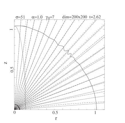
Figure 1: The steady-state relativistic plasma flow in the nearest zone of the star for the parameters $\sigma$, $\alpha$, initial Lorentz-factor $\gamma_{0}$, dimension of the lattice and duration of the simulation in units $R_{f}/v_{0}$ indicated at the top of the figure. The cylindrical coordinates $z$ (axis of rotation) and $r$ (equator) are given in units of $R_{f}$. The star is located in the lower left-hand corner of the figure. Solid lines radiating out from the star indicate the lines of the poloidal magnetic field while dashed lines represent the lines of the poloidal electric currents generated at the rotation. Thick (thin) solid lines indicate the fast (Alfvenic) mode surface, while the vertical dot-dashed line represents the light cylinder.

In Fig. 1 we show the result of the numerical simulation of the plasma outflow in the nearest zone of the star, for a time interval $t=2.62R_{f}/v_{0}$ and for the set of the values of the two key parameters, $\alpha=1.0$ and $\sigma=51$. This time interval is larger by a factor of 2.62 compared to the typical time the plasma and all MHD perturbations take to travel from the surface of the star to the fast mode surface. Note that during this time interval, a steady state solution is reached, since all perturbations which could be excited at the start of the simulation have left the box of simulation. The initial fast mode surface is circular with a radius equal to 1 in our units. Note that the final fast mode surface shown in Fig. 1 has a small amplitude kink structure at a polar angle around 45 degrees. Such a structure is formed in all simulations performed with the present method and in the present geometry (Washimi & Shibata shibata (1993), Bogovalov & Tsinganos bogts (1999)). Basically it is due to the shape of the surface of the star which is actually approximated by a sequence of step functions in the cylindrical system of coordinates.

Figure 2: The relativistic plasma flow in the far zone for $\alpha=1.0$ and $\sigma=51$. The coordinates are expressed in units of $R_{f}$.

The SC theory predicts that a wind of relativistic plasma consists of a cylindrically collimated core surrounded by a radially expanding flow (Heyvaerts & Norman heyvaerts (1989), Chiueh et al. chiueh (1991) and Bogovalov bog95 (1995)). An inspection of Fig. 1 shows that the collimation of the plasma along the axis of rotation is practically invisible in the nearest zone. The results of the same simulation in the far zone are presented in Fig. 2. At a first glance, in the far zone there is no cylindrical collimation. However, a closer examination of the results shows that a cylindrically collimated core is actually formed in the wind.

Fig. 3 gives the distribution of the poloidal magnetic field across the axis of rotation for two values of $z$. This distribution differs from that expected for a m-l wind. The m-l poloidal magnetic field is described by the equation $B_{p}=B_{0}/(r^{2}+z^{2})$. And, at a fixed $z$ the poloidal field normalized to its value at the axis of rotation ($B_{axis}$) depends on $r$ as $B_{p}/B_{axis}=1/(1+(r/z)^{2})$. Then, at $z=1121R_{f}$ the poloidal magnetic field remains practically constant at $r\leq 5\ll z=1121$. This dependence is represented by the horizontal line $B_{p}/B_{axis}=1$ in Fig. 3. However, our numerical simulation gives a totally different picture. Namely, the poloidal magnetic field has clearly a maximum at the rotation axis and then drops down with the distance $r$ from the axis, for example at $r\sim R_{f}$ to half its value from the axis. It is important that this distribution is practically independent of $z$. This result implies that the wind near the axis of rotation has achieved an asymptotic state and the flow is collimated exactly along the axis of rotation here.

The m-l model allows us to perform a quantitative comparison of the SC theory and our numerical experiment. The structure of the cylindrically collimated flow at large distances from the source is especially simple provided that the central source rotates uniformly while the plasma velocity and the ratio of the poloidal magnetic and mass fluxes (function $cF$ in Eq. (7)) are constant across the jet. In this case the dependence of $B_{p}$ on $r$ at the fixed $z$ for a cold plasma is given by the simple analytical expression (Bogovalov bog95 (1995))

$${B_{p}\over B_{0}}={1\over 1+(r/R_{j})^{2}},$$ (26)

where $R_{j}=\gamma_{j}v_{j}/\Omega=R_{f}U_{j}/U_{0}\alpha$ is the characteristic radius of the collimated flow of the cold plasma, while $\gamma_{j}$ and $v_{j}$ are the Lorentz factor and the velocity of the plasma in this flow, respectively. Eq. (26) is a direct consequence of the SC theory and is valid at $r\gg R_{l}$. The dependence of the normalised plasma density on $r$ is identical to the distribution (26) since $F$ and the plasma velocity are assumed to be constant across the cylindrically collimated flow. In this case the plasma density is simply proportional to the poloidal magnetic field, since $\rho=B_{p}/4\pi v_{p}cF(\psi)$ (see Eq. (7)).

All these conditions are indeed fulfilled in our case. The outflow speed at the vicinity of the axis of rotation is close to the speed of light ( $v_{p}=0.87c$ at $\gamma_{0}=2$ and $v_{p}=0.98c$ at $\gamma_{0}=7$) and is independent of $r$. The function $F$ is assumed independent of $\psi$ for all field lines and the star rotates uniformly. A comparison of the calculated dependence of $B_{p}$ on $r$ with the analytical prediction, Eq. (26), shows that the SC theory correctly predicts the asymptotic properties of the wind structure.

The cylindrically collimated flow in Fig. (2) is not visible since its transversal scale is extremely small. The flux of the poloidal magnetic field contained in this flow is small as well. The dependence of the magnetic flux on $r$ is shown in Fig. (3) by the dashed-dotted line. For plotting convenience, this flux is multiplied by 100 and is also normalised to the total magnetic flux in the upper hemisphere, $\psi_{eq}$, which coincides with the magnetic flux at the equator. The mass flux normalised to the total mass flux in the upper hemisphere is presented by the same curve since the mass flux is proportional to the poloidal magnetic field in our case. The fraction of the magnetic and mass flux in the cylindrically collimated flow is of the order $0.1\%$. The rest of the magnetic and mass flux expands radially, in accordance with the SC theory.

Figure 3: The distribution of the poloidal magnetic field across the jet at $z=1121R_{f}$ (solid line) and $z=140R_{f}$ (dots), compared with the prediction of analytical theory (dashed line). The poloidal magnetic field is normalized to its value at the axis, $r=0$. The dashed-dotted line gives the distribution of the ratio of the magnetic flux to the total magnetic flux in the upper hemisphere multiplied by 100. The distance to the axis of rotation $r$ is expressed in units of $R_{f}$ such that the radius of the jet is $1/\alpha=1$.

The same physical picture emerges for a larger value of $\alpha$. In Fig. (4) we show in the nearest zone the results of the simulation of the flow of plasma for $\alpha=4$.

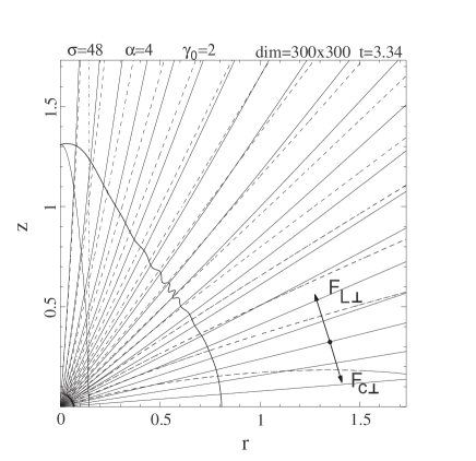
Figure 4: Steady-state relativistic plasma flow in the nearest zone of the star and for the parameters $\sigma$, $\alpha$, initial Lorentz-factor $\gamma_{0}$, dimension of the lattice and the duration of the simulation in units $R_{f}/v_{0}$ indicated at the top of the figure. Coordinates $z$ (axis of rotation) and $r$ (equator) are given in units of $R_{f}$. The star is located in the lower left-hand corner of the figure. Solid lines radiating out from the star indicate the lines of the poloidal magnetic field while dashed lines represent the lines of the poloidal electric currents generated at the rotation. Thick (thin) solid lines indicate the fast (Alfvenic) mode surface, while the vertical dot-dashed line represents the light cylinder.

The increase $\alpha$ does not change significantly the structure of the flow, although collimation now becomes visible even in the nearest zone. The same flow in the far zone is shown in Fig. (5). It may be seen from this figure that a very narrow collimated beam is formed in the wind. The structure of the cylindrically collimated flow is shown in Fig. (6) for two values of $z$.

Figure 5: Relativistic outflow in the far zone of the star for $\alpha=4$ and $\sigma=48$. The coordinates are expressed in units of $R_{f}$.

Figure 6: The dependence of the poloidal magnetic field across the jet at $z=10350R_{f}$ (solid line) and at $z=1000R_{f}$ (dotted line) compared with the prediction of analytical theory (dashed line). The poloidal magnetic field is normalized to its value at the axis, $r=0$. The dashed-dotted line gives the distribution of the ratio of the magnetic flux to the total magnetic flux in the upper hemisphere multiplied by 100. The distance to the axis of rotation $r$ is expressed in units of $R_{f}$ such that the radius of the jet is $1/\alpha=0.25$.

The efficiency of the acceleration of the plasma by a rotating object is important in astrophysical applications. This acceleration in the model under consideration is expected to be most efficient near the equatorial plane since at the axis of rotation there is no accelerating force at all. The accelerating force in the poloidal direction is proportional to the product $j_{\perp}B_{\varphi}$, where $j_{\perp}$ is the component of the electric current perpendicular to a field line. The accelerating force in the azimuthal direction is proportional to the product $j_{\perp}B_{p}$. Thus, all accelerating forces are proportional to $j_{\perp}$. This implies that the acceleration occurs only if the electric currents cross the poloidal field lines. The electric currents shown by the dashed line in Figs. (1) and (4) indeed cross the poloidal field lines. This is very well seen especially in Fig. (4) near the equator.

The dependence of the four-velocity of the plasma on the distance from the centre of the source is shown in Fig. (7). The distance is given in a logarithmic scale. The energy of the particles increases slower than logarithmically and reaches a constant value. It follows from energy conservation (10) that the maximum possible terminal four-velocity $U_{\infty}$ at the equator is $U_{\infty}=U_{0}(v_{\infty}/v_{0})\sigma$, since $W$ at the equator can be estimated as $\gamma_{0}\sigma$, provided that $\sigma\gg 1$ and the toroidal magnetic field is estimated as $B_{\varphi}\approx-r\Omega B_{p}/v_{0}$ (Bogovalov 1997a ). All Poynting flux should be transformed into kinetic energy of the plasma in this case. But this value of the velocity is never achieved. Michel (michel (1969)) calculated for $U_{\infty}$ the value $U_{michel}=(\sigma U_{0})^{1/3}$ for the plasma flow in a prescribed and fixed m-l poloidal magnetic field. Therefore, $U_{michel}/U_{0}=\alpha^{2/3}$ (see Eq. 24). It is reasonable to estimate the efficiency of the plasma acceleration as the ratio $\xi=U_{\infty}/U_{0}\sigma$ which is approximately the ratio of the part of the Poynting flux transformed into the kinetic energy of the plasma (this is valid, provided that $U_{\infty}\gg U_{0}$) to the initial value of the Poynting flux at the equator in the relativistic limit. For the Michel solution (michel (1969)) $\xi=\alpha^{2/3}/\sigma$. The same value is given by Beskin et al. (beskin98 (1998)) for the analytical solution of the same problem under the assumption that the poloidal magnetic field goes to a monopole-like field at $\alpha\rightarrow\infty$. It follows from Fig. (7) that $U_{\infty}/U_{0}$ increases with $\alpha$ essentially faster than $\alpha^{2/3}$. For the flow with $\alpha=4$ Michel’s estimate gives $U_{p,\infty}/U_{0}=2.5$, while the numerical solution gives more than 8. Correspondingly, the efficiency of the acceleration remarkably exceeds the efficiency of the acceleration given by Michel and achieves $16.7\%$ for the flow at $\alpha=4$ and $\sigma=48$. It follows from Fig. 7 that the remarkable part of the acceleration occurs at large distances from the star. It happens at the collimation of the magnetic flux to the axis of rotation due to disbalance arising between the tension and pressure gradient of the toroidal magnetic field (Begelman, & Li li (1994), Fendt & Camenzind fendt96 (1996)). This mechanism was not taken into account in the analysis of Michel (michel (1969)) and Beskin et al. (beskin98 (1998)) since they assumed a fixed m-l magnetic field.

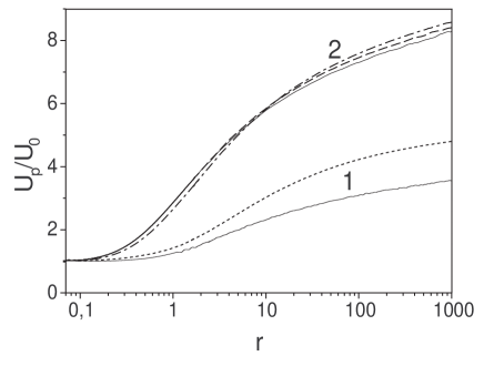
Figure 7: Dependence of $U_{p}$ along a field line on the distance to the centre of the source expressed in $R_{f}$. Curve 1 is for $\alpha=1.0$, $\sigma=51$ for the equatorial plane. Curves under number 2 are for the equatorial plane (solid line), for $\psi/\psi_{eq}=0,7$ (dashed line), for $\psi/\psi_{eq}=0,3$ (dashed-dotted line) and for $\psi/\psi_{eq}=0,03$ (dotted line) for the parameters $\alpha=4$, $\sigma=48$.

It follows from Fig. 7 that the largest energy is achieved not at the equator but at $r=1000R_{f}$ for $\alpha=4$. To understand why this happens it is convenient to look on the dependence of $U_{p}/U_{0}$ on $\psi$ across field lines. This dependence is presented in Fig. (8) by two upper curves 1 ( for $z=1000R_{f}$) and 2 (for $z=10350R_{f}$). These curves have small amplitude irregular structure which is purely of numerical origin. It arises at large distances where the program deals with large numbers. The maximum of the acceleration is achieved not at the equator, but at $\psi/\psi_{eq}\sim 0.3$. This is explained by the fact that the asymptotical regime predicted by the SC theory is actually not achieved at these $z$ for $\psi/\psi_{eq}>0.05$. It appears that the larger $\psi$ the larger the distance which is necessary to reach the asymptotic regime of the outflow. This property of the SC process has already been found in the nonrelativistic outflow simulation (Bogovalov & Tsinganos bogts (1999)).

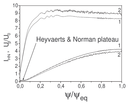
Figure 8: Dependence of the four-velocity of the plasma $U_{p}/U_{0}$ (upper curves) and Heyvaerts & Norman integral ${\rm I}_{HN}$ (lower curves) on $\psi$ for $z=1000R_{f}$ (curve 1) and $z=10350R_{f}$ (curve 2). The parameters of the outflow are $\alpha=4$, $\sigma=48$, $\gamma_{0}=2$.

The physics of this phenomena can be understood as follows. It can be shown from simple geometrical consideration that

$${1\over g_{\eta}}{\partial g_{\eta}\over\partial\psi}={1\over rR_{c}B_{p}}\,,$$ (27)

where $R_{c}$ is the curvature radius of the poloidal magnetic field lines, with $R_{c}$ positive if the centre of curvature is in the domain between the line and the axis of rotation and negative in the opposite case. With this expression, Eq. (13) takes the form

$$\begin{array}[]{c}{\partial\over\partial\psi}\left[{B_{p}^{2}\over 8\pi}\right]+{1\over 8\pi r^{2}}{\partial\over\partial\psi}\left[r^{2}(B^{2}_{\varphi}-E^{2})\right]-{1\over 4\pi r}\left[{\partial r\over\partial\psi}\right]{U_{\varphi}^{2}B_{p}\over U_{p}F(\psi)}\\ \\ -{[U_{p}-F(\psi)(1-(r\Omega/c)^{2})B_{p}]\over 4\pi rR_{c}F(\psi)}=0.\end{array}$$ (28)

Let us consider the flow in the region of radial expansion, as in the case under consideration, where the SC is small. For simplicity, we neglect the acceleration of the plasma. The first term in this equation decreases with $r$ as $r^{-4}$. The second one decreases as $r^{-2}$, since $B_{\varphi}\sim E\sim rB_{p}$ (Bogovalov 1997a ). The third term is proportional to the product $rU_{\varphi}^{2}B_{p}$. This term decreases as $r^{-3}$, since $rB_{p}\sim 1/r$ and $U_{\varphi}\sim 1/r$ due to angular momentum conservation. Thus, only the second and fourth terms survive in Eq. (28) at these large distances. Therefore, this equation takes the form

$${1\over 8\pi x^{2}}{\partial\over\partial\psi}(x^{2}(B^{2}_{\varphi}-E^{2}))-{(U_{p}+F(\psi)x^{2}B_{p})\over 4\pi xR_{c}F(\psi)}=0,$$ (29)

where $x=r\Omega/c$. From the frozen-in condition (2) we may estimate the toroidal magnetic field at large distances when $v_{\varphi}\rightarrow 0$, where $v_{\phi}$ is the azimuthal velocity.

$$B_{\varphi}=-{Ec\over v}.$$ (30)

In the asymptotic regime plasma moves along straight lines, when $R_{c}\rightarrow\infty$. The structure of the flow in this regime is defined by the trivial equation

$${\partial\over\partial\psi}(x^{2}(B^{2}_{\varphi}-E^{2}))=0.$$ (31)

Together with Eq. (30) this equation gives that the relativistic generalization of the Heyvaerts & Norman integral $I_{HN}=|xB_{\varphi}|/\gamma$ (Chiueh et al. chiueh (1991)) should be constant in the region of radial expansion. This integral, shown in Fig. (8) by the two lower curves for essentially different distances, is actually constant in the small region $0.01<\psi/\psi_{eq}<0.05$ (Heyvaerts & Norman plateau in the figure). But at $\psi/\psi_{eq}>0.05$, $I_{HN}$ is not constant. This contradicts the expected behavior of $I_{NH}$, but, as we show below, this implies that the asymptotic regime is still not reached in this region of $\psi$.

The characteristic scale of collimation $D_{coll}$ which defines the distance where the flow reaches the asymptotic regime can be estimated as follows. $d\theta/dR=1/R_{c}$, where $\theta$ is the polar angle of the plasma velocity and $R$ is the distance to the center of the source. In the radially expanding wind $d\psi=B_{p}r^{2}\sin(\theta)d\theta$. Taking into account also that at large distances $B_{\varphi}=-(r\Omega/v_{p})B_{p}$ (Bogovalov 1997a ), the rate of turning of the trajectory of the plasma follows from Eq. (29) and is defined by the equation

$$|{d\theta\over dR}|\leq{\sin{2\theta}\over RU_{0}^{2}({1\over\sigma}+\sin^{2}{\theta})}.$$ (32)

Integration of this equation gives the estimate of the distance at which the line of the flow turns through the angle $\Delta\theta$. The scale of the collimation of the flow line $D_{coll}$ is defined by the distance at which the flow line turns through the angle $\Delta\theta\sim\theta$. The integration of equation (32) can be performed from the fast mode surface since this consideration is valid only in the supersonic region. The scale of the collimation is estimated as

$$D_{coll}\geq R_{f}\exp\left[{\theta U_{0}^{2}({1\over\sigma}+\sin^{2}\theta)\over\sin 2\theta}\right]\,.$$ (33)

According to this equation there are two regions of the flow with the essentially different dependence of $D_{coll}$ on the parameters of the flow. The smallest $D_{coll}$ takes place for small angles limited by the value $\theta^{2}<1/\sigma$. For these angles the scale of the collimation is (see also Bogovalov & Tsinganos bogts (1999))

$$D_{coll}\geq R_{f}\exp{1\over 2\alpha^{2}}.$$ (34)

Similar to the nonrelativistic outflow the collimation of the plasma close to the rotational axis occurs near the fast mode surface at $\alpha>1$. At the initially m-l outflow the magnetic flux depends on the angle $\theta$ as $\psi=\psi_{eq}(1-\cos\theta)$. Therefore, the part of the magnetic flux where the collimation occurs as in the nonrelativistic limit is

$${\psi\over\psi_{eq}}\leq{1\over 2\sigma}.$$ (35)

The collimation scale of the other part of the flow ( at low latitudes) is defined by the equation

$$D_{coll}\geq R_{f}\exp{\theta\sin\theta U_{0}^{2}\over 2\cos\theta}.$$ (36)

and at the angles $\theta^{2}\gg 2/U_{0}^{2}$ the collimation scale becomes large compared with $R_{f}$ independent of $\sigma$. It follows from this result that the remarkable bend of the flow lines at low latitudes is possible only for the plasma with relatively low $U_{0}$. The collimation scale increases exponentially with the growth of the Lorentz factor of the plasma. These properties of the flow explain the numerical results.

In the simulation we obtain such a behavior of the flow, with three regimes: a core where the current increases with $\psi$, the Heyvaerts & Norman regime and the regime where the enclosed current increases (Fig. 8). Thus, an extremely narrow cylindrical core is formed which contains the magnetic flux $\psi<(1/2\sigma)\psi_{eq}$. This core is formed at a distance comparable to $R_{f}$ for $\alpha>1$, similarly to the nonrelativistic limit. For larger $\psi$ the collimation scale is defined by Eq. (36). For $\gamma_{0}=7$ the characteristic scale of collimation is of the order of $R_{f}\cdot 10^{10.6\theta\tan\theta}$. It implies that the smaller $\theta$, the earlier the asymptotic regime will be achieved. This explains why the Heyvaerts & Norman plateau is formed only at the relatively small $\theta$ (small $\psi$). At larger $\theta$ the scale of collimation exponentially increases and finally diverges at $\theta=\pi/2$. Thus, the asymptotic regime cannot be achieved at low latitudes. At the final distance from the source there should exist a region at low latitudes (large $\psi$) where $I_{NH}$ is not constant. It is this behavior which is found in our calculations.

For $\alpha=4$ the collimation is more efficient and the effect of collimation appears already in the nearest zone where the plasma is not yet accelerated. At the estimation of the collimation scale it is necessary to take into account acceleration of the plasma to a Lorentz factor greater than 10 near the equator. This could be done by integration of Eq. (32) from a radius $R_{in}>R_{f}$ where the energy of the plasma practically reaches the terminal value. If we take into account the acceleration, the asymptotic regime (in which $I_{NH}$ does not depend on $\psi$ in a radially expanding wind) will be achieved at a distance of the order $D_{coll}>R_{f}10^{22\cdot\theta\tan\theta}$. It follows from this expression that at $\alpha=4$ the asymptotic regime at $R\approx 10^{4}\cdot R_{f}$ will be achieved only for $\psi/\psi_{eq}<0.1$. This value agrees well with the numerical results presented in Fig. 8 in the limits of uncertainties.

Comparison of the present work with our previous work (Bogovalov & Tsinganos bogts (1999) ) shows that the relativistic plasma is collimated less efficiently than the nonrelativistic one. In particular, the fraction of the collimated mass flux in the nonrelativistic flow was close to $1\%$, while in the relativistic limit it is of the order $0.1\%$. This difference can be understood from simple qualitative consideration. The dynamics of the cold plasma is basically controlled by two forces. One of them is the volumetric Lorenz force, $({\bf j}\times{\bf B})/c$ and the other is the volumetric Coulomb force, $q\bf E$ (see Eq.(1)). The collimation of the plasma to the axis of rotation is defined by the components of these forces perpendicular to the stream lines. The perpendicular component of the Lorenz force is $F_{L\perp}={1\over c}j_{\parallel}B_{\varphi}$, where $j_{\parallel}$ is the component of the poloidal electric current parallel to the poloidal magnetic field and $B_{\varphi}$ is the toroidal magnetic field. The perpendicular component of the Coulomb force is $F_{C\perp}=q\cdot E_{\perp}$. These forces are shown schematically in Fig. (4). It is important to note that these two forces are directed along opposite directions. The Lorenz force collimates the plasma while the Coulomb force decollimates it. In the nonrelativistic limit the Coulomb force is neglected, since it is negligible in comparison to the Lorenz force. The ratio of the Coulomb and Lorenz forces is of the order $(v/c)^{2}$ in this limit. In the relativistic limit the Coulomb force becomes practically equal to the Lorenz force and it strongly decreases the SC of the plasma. That is why the relativistic generalization of the parameter $\alpha$ introduced earlier for the nonrelativistic winds (Bogovalov & Tsinganos bogts (1999)) has additionally the Lorentz factor in the denominator (see Eq. (23)).

Although the Lorentz factor in the denominator of Eq. (23) decreases remarkably the value of $\alpha$, it was expected that the collimation of the relativistic plasma will be strong enough at the condition $\alpha>1$. In the nonrelativistic case the collimation becomes strong already in the subsonic region under this condition. The most surprising result is that the relativistic plasma is practically not collimated, even under this condition. The increase of the collimating force does not provide more efficient collimation of the relativistic plasma! This happens since another relativistic effect comes into play.

The curvature $\kappa_{c}=1/R_{c}$ of the stream lines of the nonrelativistic plasma is defined by the simple equation

$$\kappa_{c}={F_{\perp}\over mnv^{2}},$$ (37)

where $m$ is mass of particles, $F_{\perp}$ is the sum of all forces affecting the plasma perpendicular to the stream line. It is seen from this equation that an increase of the force $F_{\perp}$ results in an increase of $\kappa_{c}$, such that collimation becomes stronger. In other words, as it is evident from Eq. (37), $\kappa_{c}$ is proportional to the collimating force and inversly proportional to the mass density of the outflowing plasma. The situation changes essentially in the case of the relativistic, Poynting dominated plasma ($\sigma>1$) where the energy flux is dominated by the electromagnetic field. Then, according to the familiar relationship between energy and mass (${\it E}=mc^{2}$), the flux of the energy is equivalent to some inertial mass flux. It follows from Eq.(29) that eq. (37) for the relativistic Poynting-dominated plasma is modified as follows

$$\kappa_{c}={F_{\perp}\over nv^{2}\gamma(m+{B_{\varphi}^{2}\over 4\pi nc^{2}})}.$$ (38)

This equation demonstrates that the effective mass of the Poynting- dominated plasma is dominated by the toroidal magnetic field. It is important that now the effective mass increases by a term proportional to $B_{\varphi}^{2}$. The collimating force is also proportional to the same term (see eq. (29)). Therefore, the increase of the collimating force is accompanied by a corresponding increase of the effective mass density of the plasma. This in turn results in the fact that the curvature $\kappa_{c}$ of the stream lines does not increase with the increase of the collimating force. This is the reason why the collimation scale (36) at low latitudes does not depend on the magnetic field and angular velocity of the source.

6 Conclusion

This work shows that the self-collimation (SC) process occurs in relativistic winds as predicted by the SC theory. The wind consists of a radially expanding part which surrounds a cylindrically collimated flow. The radius of the cylindrically collimated flow is $R_{j}\approx R_{f}/\alpha$, where $R_{f}$ is the initial radius of the fast magnetosonic surface. The mass flux in the collimated part is small compared with the total mass flux in the wind ($\sim 10^{-3}$), even for relatively small Lorentz factors. SC essentially decreases for larger Lorentz factors. Acceleration of the plasma occurs in the radially expanding wind while the plasma in the jet is not accelerated in this cold outflow model.

The relatively small part of the mass flux in the cylindrically collimated flow has been also found in our simulations of nonrelativistic outflows (Bogovalov & Tsinganos bogts (1999)), although the magnetic flux contained in the relativistic case appears smaller by a factor of order 10. In addition, the collimation scale at low latitudes does not depend on the magnetic field and the angular velocity of the central source for $\alpha>1$, in contrast with our results for the nonrelativistic winds in the same model. This means that the weak collimation of the relativistic plasma is due to the intrinsic property of the plasma and not to a property of the model. Collimation decreases due to the affect of the electric force which becomes comparable with the collimating Lorenz force in the relativistic

limit and in the high $\sigma$ limit the collimation is saturated due to the contribution of the electromagnetic field into the inertial mass of plasma.

The most striking feature of the collimated flows obtained in the model under consideration is that a very small fraction ($\sim 10^{-3}$) of the mass flux exists in the collimated flow in comparison to the mass flux in the wind. This result is apparently in conflict with observations of AGN. The source of the wind energy is the gravitational energy released by the accreted matter. Therefore, the energy flux in the wind should be less than the luminosity of the accretion disk where about half of the gravitational energy is released (Shakura & Sunyaev ss (1973)). The total luminosity of AGN $L_{tot}$ in soft electromagnetic emission ( below X-rays) should be comparable with the energy released at the accretion. According to our results the energy flux in the jet $\dot{E}_{jet}$ should be by the factor $10^{-3}$ less than the accretion energy, $\dot{E}_{jet}<10^{-3}\cdot L_{tot}$. This disagrees with observations. X-ray and gamma-ray emission is usually attributed to the emission from jets (Urry & Padovani urry (1995)). Sometimes, the luminosity of the jets is less only by a factor of 10 than the total luminosity of AGN at other wavelengths (Elvis et al. elvis (1994)). The energy flux in this emission can be considered as the lower limit on the energy flux in the jet (however, we do not take into account beaming here). If so, we have in AGN $\dot{E}_{jet}>10^{-1}\cdot L_{total}$.

This disagreement between theory and observations implies that either the present model has no observed counterpart or the SC mechanism is not able in principle to provide collimation of the major fraction of the outflow into the jet. It is important in this regard to understand from the theoretical point of view what modifications should be made in order to provide magnetic collimation of the major fraction of the relativistic wind. This problem has been already investigated by Bogovalov & Tsinganos (bogts00 (2001)) in relation to nonrelativistic winds. It was shown in this study that in a model consisting of a central source ejecting a high-speed wind and an accretion disk ejecting a nonrelativistic magnetised outflow, all the mass flux from the central source can be cylindrically collimated indirectly by the surrounding disk-wind. Apparently, a collimation of the major part of a relativistic outflow from a central source can be provided by the same mechanism in the context of the present model as well.

Appendix A Details of the numerical simulation in the nearest zone.

For the numerical solution of the time dependent problem, the system of equations should be presented as

$${\partial\over\partial t}\hat{\Phi}=A(\hat{\Phi},\hat{\Phi}_{i},\hat{\Phi}_{ik}),$$ (39)

where $\hat{\Phi}$ is the vector of the plasma state which includes the density, components of the velocities and magnetic fields. $\hat{\Phi}_{i}$ and $\hat{\Phi}_{ik}$ are the first and the second order derivatives of $\hat{\Phi}$ on the spatial variables. Eq. (1) contains the time derivative $\bf\dot{E}$ in the right hand part generated by the displacement current in Eq. (3). Therefore, some special transformation of Eq. (1) is necessary to get form (39). The specific form of this transformation is not unique. In our previous work (Bogovalov 1997a ) unsuccessful choice of this transformation resulted in the instability of the numerical code in the Poynting flux-dominated regime. Here we use another form of the equation of motion which provides stable numerical code in all regimes.

This equation can be obtained as follows. Time derivative of the frozen-in condition (2) gives that

$${\bf\dot{E}}=-{1\over\gamma}({\bf\dot{U}\times B})-{1\over\gamma}({\bf U\times\dot{B}})-{\dot{\gamma}\over\gamma}{\bf E}.$$ (40)

Substitution of Eq. (40) and Eq. (3) together with the relativistic relationship $\dot{\gamma}=v_{i}\dot{U}_{i}/c$ in Eq. (1) gives the equation of motion in the form

$$M_{ik}\dot{U}_{k}=-\rho({\bf v\cdot\nabla})U_{i}+qE_{i}/c+{1\over 4\pi c}(({\bf\nabla\times B)\times B})_{i}$$ (41)

$$-{1\over 4\pi c^{3}}(v_{i}({\bf B\cdot\dot{B}})-\dot{B}_{i}({\bf B\cdot v})),$$

where

$$M_{ik}=(\rho+{B^{2}\over 4\pi c^{2}\gamma})\delta_{ik}-{1\over 4\pi c^{2}\gamma}(B_{i}B_{k}+S_{i}v_{k}/c)$$

and $S_{i}=({\bf E\times B})_{i}$. Terms with $\bf\dot{B}$ in the right hand part of Eq. (41) are eliminated with help of Eq. (4). After that, multiplication of equation of motion (41) on the inverse matrix

$$M_{ik}^{-1}={1\over(\rho+{B^{2}\over 4\pi c^{2}\gamma})}[\delta_{ik}+$$ (42)

$${B_{i}B_{k}\over 4\pi\rho c^{2}\gamma}+{({\bf v\cdot B}/c)S_{i}B_{k}/4\pi\rho c^{2}\gamma+S_{i}v_{k}/c\over(4\pi\rho c^{2}\gamma+B^{2}-({\bf S\cdot v}/c)}]$$

gives the equation of motion in the form (39) appropriate for the numerical solution.

A two-step Lax-Wendroff numerical scheme was used for the numerical solution of the problem (Press et al. press (1990)). The analytical solution obtained for the slow rotators (Bogovalov 1997a ) was used as the initial state of the plasma.

The testing of the numerical code was performed by comparison of the results with the results obtained with the nonrelativistic version of the code (Bogovalov & Tsinganos bogts (1999)), by comparison with predictions of the analytical theory (Bogovalov bog92 (1992), Bogovalov 1997a ) and by simulation of the perturbation propagation in the wind. One of these tests is presented in Fig. 9. The beginning of the star rotation starts the shock wave propagating with the Alfvenic velocity in the isotropic wind. This velocity is very close to 1 for the taken parameters of the wind. The shock has an oscillating structure typical for the collisionless shocks. The front is smoothed due to the numerical diffusion. The first (largest) maximum can be accepted as the boundary of the shock. It follows from the figure that the wave propagates with the velocity very close to the light velocity which is equal $c/v_{0}=1.01$ in the dimensionless variables normalized to $v_{0}$ at $\gamma_{0}=7$.

Figure 9: The simulation of propagation of the switch on shock wave in the relativistic wind. All the notations are the same as in Fig. 1 and 4. The wave is generated at the beginning of rotation of the central object.