Layer Formation in Semiconvection

Abstract

Layer formation in a thermally destabilized fluid with stable density gradient has been observed in laboratory experiments and has been proposed as a mechanism for mixing molecular weight in late stages of stellar evolution in regions which are unstable to semiconvection. It is not yet known whether such layers can exist in a very low viscosity fluid: this work undertakes to address that question. Layering is simulated numerically both at high Prandtl number (relevant to the laboratory) in order to describe the onset of layering intability, and the astrophysically important case of low Prandtl number. It is argued that the critical stability parameter for interfaces between layers, the Richardson number, increases with decreasing Prandtl number. Throughout the simulations the fluid has a tendency to form large scale flows in the first convecting layer, but only at low Prandtl number do such structures have dramatic consequences for layering. These flows are shown to drive large interfacial waves whose breaking contributes to significant mixing across the interface. An effective diffusion coefficient is determined from the simulation and is shown to be much greater than the predictions of both an enhanced diffusion model and one which specifically incorporates wave breaking. The results further suggest that molecular weight gradient interfaces are ineffective barriers to mixing even when specified as initial conditions, such as would arise when a compositional gradient is redistributed by another mechanism than buoyancy, such as rotation or internal waves.

1 Introduction

Though semiconvection may be an important mechanism for mixing of chemicals in late stages of stellar evolution, there have been few numerical simulations of semiconvective scenarios. In part, this is due to the fact that the numerical resolution required for a simulation has, until recently, made computation prohibitive. Coupled to that, the fact that the existing mixing length theories (such as Stevenson (1979), Langer et al. (1983) and Spruit (1992)) which both draw on theoretical and experimental arguments, seemed adequate when compared to observations.

However, recent observations of SN1987A have been at odds with models of late stages of stellar evolution and one main suspect are the theories of elemental mixing used in those models (Maeder & Conti (1994)). As with all turbulence models, the more sophisticated semiconvective models (Canuto (1999), Grossman (1996), Grossman et al. (1993)) which arose in the wake of these new data require closure assumptions. Implicit in these are assumptions about the character of the flow which have yet to be tested against numerical experiments of semiconvection. Numerical simulations are now sophisticated enough that we can hope to distinguish between the assumptions made in the mixing length theories and settle the question of the heat transport, chemical mixing and velocity field associated with semiconvective zones. In this work, I shall address one particular question related to all three of these topics: does layered convection develop when a compositionally stratified fluid, with very low viscosity, is subjected to a vertical heat flux?

1.1 Semiconvection and Double Diffusion

Kato (1966a) performed a local analysis of the convective instability of gases with a varying compositional gradient subjected to an upward heat flux and showed three criteria for instability. If the molecular weight increases upward, $d\mu/dz>0$, the fluid is unstable to the Rayleigh-Taylor instability. If

$$\nabla_{rad}>\nabla_{Led}=\nabla_{ad}+\frac{\beta}{4-3\beta}\nabla_{\mu}$$ (1)

then the fluid is exponentially unstable to classical convection. Here, $\nabla_{ad}$ is the adiabatic temperature gradient, $\nabla_{ad}=(\partial\ln T/\partial\ln p)_{S}$ and $\nabla_{rad}$ is the corresponding temperature derivative due to radiative diffusion. $\nabla_{\mu}=\partial\ln\mu/\partial\ln p$, $\mu$ is the molecular weight and $\beta$ is the ratio of gas pressure to the total pressure. This criterion was discovered by Ledoux (1947) and bears his name. Finally, Kato demonstrated that when

$$\nabla_{ad}<\nabla_{rad}<\nabla_{Led}$$ (2)

convection sets in through overstable oscillations. The physical explanation of this instability requires considering blobs of fluid rising in a hydrostatically stratified medium. If the medium is stable to the Ledoux criterion, such blobs will fall back to their initial positions. If, further, we allow heat to diffuse from the blobs (by far the fastest diffusing process in astrophysical contexts) then the returning blobs will have lost a small amount of heat on their round trip and will overshoot their initial positions. This mechanism relies on the existence of thermal diffusion and the growth rate of overstable modes is in fact proportional to the thermal diffusivity. Thus, overstable convection grows much more slowly than classical thermal convection and it would be reasonable to expect that the convection, itself, is less vigorous than its classical counterpart.

The weakness of linear oscillatory convection may be a completely irrelevant fact since the bifurcation that leads to overstability is subcritical. That is to say, the fluid can go unstable to small, but finite amplitude perturbations, at values of the temperature gradient far below that required for overstability. This is a weakly non-linear effect and is due to the fact that a small rearrangement in the molecular weight (due to breaking gravity waves, shear instability, etc) can drive the fluid to classical thermal convection, since the stabilizing compositional gradient may be locally destroyed.

Weakly non-linear analysis was performed by Veronis (1968) for an incompressible, Boussinesq fluid with a stabilizing salt gradient and destabilizing temperature gradient. Though superficially appropriate for only the oceanographic situation for which it was derived, it was pointed out by E.A. Spiegel (see Kato (1966a)) that the linear stability equations of semiconvection are equivalent to the incompressible equations with the salt playing the role the molecular weight. In the oceanographic context such overstability is referred to as double diffusion.

The effect of the redistribution of the stabilizing component is most dramatically seen in the now famous experiment by Turner & Stommel (1964) and reproduced by Turner (1968), Huppert & Linden (1979) and Fernando (1987) and Fernando (1989). In the prototype and all of its successors, a tank of water with a stable salinity concentration gradient is heated from below. At first the water becomes unstable to rapidly rising convective plumes but, since they are rising into a region of less salt concentration, the plumes are restricted to a thin region at the bottom of the tank. The salt is rapidly mixed thus there is no gradient in this region and the fluid motion becomes turbulent. Subsequently, the layer proceeds to slowly entrain from the nonconvecting fluid above it while transporting heat to that region and at all times increasing in temperature. After a critical layer thickness is reached, the boundary layer separating the convecting fluid from the quiescent fluid above is seen to undergo oscillatory instability. This, in turn, redistributes the salt in the second convecting layer which is now separated from the first by a buoyancy jump. The convection becomes turbulent in this second layer and the process continues in subsequent layers. At intermediate times, the tank has formed a vertical stack of convecting layers with well mixed temperature and salt within each. Though mixing between layers is limited by the saline density jump across each, the lower layers are able to slowly erode this density jump over much longer time scales by the breaking of internal waves on the interfaces between the layers.

Fernando (1987) & Fernando (1989), provide the most accurate quantitative data for the water-salt experiment. In particular, he confirms the existing theory for the development of the first layer and gives a criterion for the stability of a layer. Defining $l$ as the integral length scale of the turbulence, the scale at which the turbulence is forced, $u_{*}$ as the root mean square turbulent velocity in the convecting layer, $\rho_{*}$, the average density of the convecting layer and $\Delta b=g(\Delta\rho)$ as the buoyancy contrast between the convecting layer and the fluid above, then

$$Ri=\frac{l\,\Delta b}{\rho_{*}u_{*}^{2}}$$ (3)

is the Richardson number of the flow. This parameter generally arises in the study of a stable buoyancy gradient in the presence of a horizontal shear flow. In the layered convection case it amounts to the ratio of the potential energy difference over the scale of the largest eddies in the turbulent flow to the kinetic energy of the flow. Fernando showed that, in the case of water-salt experiment, there are three regimes of interest delimited by the Richardson number.

At low Richardson numbers, the turbulent eddies are able to penetrate deeply into the static fluid and the interface migrates upward. At intermediate Richardson numbers, mixing across the stable density interface is primarily due to the breaking of interfacial (internal) waves and the scouring of this surface by a weaker flow that can be maintained in the upper fluid. At higher Richardson number, the effect of interfacial waves and penetration becomes negligible as convective plumes flatten out when they hit the density interface. Transport across the layers then takes place purely by diffusion, though enhanced by the steep gradient at the interface.

Only when the Richardson number, based on the uppermost layer and the static fluid, is of intermediate or high values does there develop an oscillatory instability in the boundary between those two regions: another layer forms.

Let us now return to astrophysical semiconvection, contrasting the semiconvective theories of Spruit (1992) and Stevenson (1979). Using the intuition of the laboratory experiments, Spruit constructed a mixing length theory of layered convection separated by thin molecular weight gradients and thicker thermal gradients. Transport across the layers is solely due to diffusion through the thin thermal and helium transition regions at the interfaces of the layers. In fact, this theory is similar to the double diffusive theory constructed for confined geometries by Knobloch & Merryfield (1992). However, confined geometries cannot support surface waves like the internal waves in layered convection and these could contribute to even greater cross interface transport.

Stevenson (1979) described a theory of semiconvection in which growing overstable modes resonantly feed energy to smaller scales and eventually break, whereupon the molecular weight gradient is redistributed. By making reference to the salt-water experiments and energetic arguments for double diffusive convection, he compellingly argued that, should layers form as a result of this wave breaking, they would be unstable if $Pr<\tau^{1/2}$. The Prandtl number, defined as $Pr=\nu/\kappa_{T}$, and the Lewis number, $\tau=\kappa_{He}/\kappa_{T}$, are ratios of the kinematic viscosity and molecular diffusivity of the second species to the thermal diffusivity, respectively. (The two species are helium in a hydrogen convection zone.) In semiconvection, the thermal diffusivity is dominated by radiation whereas both viscosity and helium diffusion are molecular processes and, as such, $1\gg Pr>\tau$. In contrast to Spruit, Stevenson’s theory would lead to the conclusion that layers are dynamically unimportant in stellar evolution.

Further evidence of layer instability is provided by the only numerical experiment on semiconvection to date, Merryfield (1995). Using the anelastic approximation for a two dimensional fluid, Merryfield studied the onset of overstable oscillations in a low Prandtl number fluid: the thermal parameters that he used put the simulations within the regime of equation (2). Although motion set in though overstable oscillations and the compositional gradient was seen to mix through the breaking of internal waves, these tended to occur on length scales comparable to the domain, and layers did not form. In one of the experiments, an initial condition of two layers separated by a stable density interface was simulated. The interface became quickly unstable to internal waves, disrupting the layers and leading to well mixed, global thermal convection. As yet, layers have not been observed to form, much less be stable, in any semiconvective simulation at low Prandtl number.

On the other hand, layers have been observed to form in a numerical experiment tailored to explaining the observations of Huppert & Linden (1979) and Fernando (1989). Molemaker & Dykstra (1997) considered an incompressible fluid at $Pr=7$ (water) with vertical salinity gradient subjected to cooling from above. Due to Boussinesq symmetry, this is completely equivalent to heating from below as is done in laboratory experiments. The numerical simulation well reproduced the observations of Fernando (1989) and confirmed the measurement of a critical Richardson number delineating the transition from layer growth by entrainment to quasi-static convective layers separated by diffusive interfaces.

1.2 Current Work

The numerical and theoretical evidence provided thus far verifies the formation of layers in the high Prandtl number regime appropriate for water. However, the results for low Prandtl number are still inconclusive. Does a multiple layered structure form in the low Prandtl number regime? If so, how does the critical Richardson number depend on Prandtl number?

The formation of a second layer above the first requires a quiescent thermal boundary layer separating the convective zone from the static fluid. In this thermal boundary the slow oscillatory instability can incubate and grow before convective erosion from below becomes significant. A smaller Prandtl number means that the viscous boundary layers separating static from convective zones is smaller than the thermal boundary layer. Convective plumes will tend to decelerate less before reaching the buoyancy interface and be able to penetrate more energetically. Smaller Prandtl number also means smaller scales for kinetic energy dissipation. The interfacial waves which are generated by the convective plumes will tend to break at smaller wavelengths. The interfacial waves will then be more effective at mixing the composition gradient across the interfaces. Both the energetic waves and smaller scale breaking tend to suppress the growth of oscillatory instability in the static fluid.

In the present work I present results of two dimensional numerical simulations of a fully compressible fluid. The molecular weight of the medium decreases upward and the diffusivity of the second species is always small. Results for successively decreasing Prandtl number and at different values of the heat flux are compared.

In section 2 the equations, choice of parameters and numerical technique are presented. The results of the simulations are presented and described in §3 and these results are compared to previous mixing length theories and numerical simulations in §4. In §5 the results are interpreted in the context of stellar models.

2 Formulation of the problem

2.1 Equations and Boundary Conditions

This work attempts to bridge the divide between terrestrial double-diffusive convection and stellar semiconvection simulations. To this end I have, at times, neglected certain processes which are less relevant to the formation and disruption of layers, though they are obviously present in realistic stars. Radiation pressure tends to decrease the contrast between the semiconvective and convective stability thresholds (equations 1, 2) and would correspondingly mitigate layer formation. Although radiation pressure is not negligible in stellar convection, for the purposes of this work, it has been neglected. This serves the added purpose of singling out differences between astrophysical and terrestrial double diffusion, since the ideal gas equation of state at constant pressure tends to the Boussinesq approximation for incompressible fluids. Any formation of layers in the present simulations can be seen as a necessary, but not sufficient condition for them to form in stars.

The equations of mass, momentum, energy and helium concentration conservation which govern a compressible fluid of hydrogen gas with a varying concentration of helium, $Y$, are (Spiegel & Veronis (1960))

$$\frac{\partial\rho}{\partial t}=-\nabla\cdot(\rho{\bf v})$$ (4)

$$\rho\left(\frac{\partial\bf v}{\partial t}+({\bf v}\cdot{\bf\nabla}){\bf v}\right)=-{\bf\nabla}p+{\bf g}\rho+\nu\rho\left(\nabla^{2}{\bf v}+\frac{1}{3}{\bf\nabla}(\nabla\cdot{\bf v})\right)$$ (5)

$$\rho~{}C_{v}\left(\frac{\partial T}{\partial t}+{\bf v}\cdot{\bf\nabla}T\right)=-p(\nabla\cdot{\bf v})+\nabla\cdot(\kappa\nabla T)+\nu\rho(\nabla\cdot({\bf v\cdot\nabla v})-\frac{2}{3}(\nabla\cdot{\bf v})^{2})$$ (6)

$$\frac{\partial Y}{\partial t}+{\bf v}\cdot{\bf\nabla}Y=\frac{\kappa_{He}}{\rho}\nabla\cdot({\rho{\bf\nabla}Y})$$ (7)

$$p=\frac{\rho RT}{\mu},$$ (8)

where $\nu,\,\kappa,\,\kappa_{He}$ are the constant kinematic viscosity, thermal diffusivity and helium molecular diffusivity, respectively. $R$ is the gas constant, $\mu(Y)$ is the molecular weight for an ionized gas of hydrogen and helium

$$\mu=(2-\frac{5}{4}Y)^{-1}$$ (9)

and the specific heat at constant volume is

$$C_{v}=\frac{3}{2}\frac{R}{\mu}.$$ (10)

Computations are performed on a rectangular box of vertical dimension, $d$ and horizontal dimension $\lambda d$ with downward directed, constant gravity. The initial conditions for the simulations are constant, negative helium gradient throughout the domain. In the bulk of the domain the temperature is chosen such that the fluid is only marginally unstable to the Schwarzschild criterion but very stable according to Ledoux.

An additional heat flux is supplied at the bottom of the domain and the temperature gradient is continuously set to match it, exponentially, over a very thin region. This has the effect of increasing $\nabla_{ad}$ to the point where the fluid is significantly unstable in a thin region at the bottom. This transition region is necessary in order to avoid any numerical instabilities which arise from impulsive heating.

In all examples, the helium concentration varies from $Y=1$ at the bottom of the domain linearly to $Y=0$ at the top.

The side boundaries are periodic while the following top and bottom boundary conditions are used,

$$v_{z}=\partial_{z}v_{x}=0 {\rm at} z=0,d$$ (11)

$$\partial_{z}Y=0 {\rm at} z=0,d$$ (12)

$$\partial_{z}T=\alpha {\rm at} z=d$$ (13)

$$\partial_{z}T=-(\alpha+F) {\rm at} z=0.$$ (14)

Physically, the velocity boundary conditions correspond to impenetrable, stress free boundaries. The helium boundary conditions are chosen so that, when convection sets in, there will not be sharp boundary layers between the convective region and the boundaries. Such layers would be computationally expensive to resolve and be irrelevant to the physics. The initial temperature profile is given by $T(z,x,t=0)=T_{d}-\alpha(z-d)+Fz_{*}e^{-\frac{z}{z_{*}}}$ where $\alpha$ and $F$ are both positive and $z_{*}\ll d$. $z_{*}$ is chosen so that the thermal boundary layer at the bottom is very thin and the temperature at the lower boundary is dominated by the $Fz_{*}$ term in the initial condition. That the heat flux is so low at the top boundary may seem to be cause for concern, since the driven convection will continue to accumulate energy faster than it can dissipate it from the top boundary. In practice, if the temperature changes significantly at the top boundary, it is due to the fact that a convective plume has arrived from the lower boundary. In such circumstances, there is no layer formation in the domain (only global thermal convection) and the simulations are stopped.

2.2 Numerical Method

The code is based on one developed by Rubini et al. (1997) and employs a mixed spatial scheme: a psuedo spectral, periodic routine in the horizontal direction and $6^{th}$ order compact finite difference in the vertical direction. The latter is more appropriate for the boundary conditions under consideration and the accuracy of the derivatives is very close to the spectral accuracy of the horizontal derivatives if double the resolution is used.

The time step for low Mach number compressible simulations is limited by the CFL condition for sound waves, $\Delta t<\Delta x/c_{s}$ where $\Delta x$ is the mesh spacing and $c_{s}$ is the sound speed. The condition corresponds to the requirement that sound waves must be tracked across each grid element. In all cases considered here, this condition is more restrictive than the corresponding condition for thermal diffusion, $\Delta t<(\Delta x)^{2}/\kappa$. Since sound waves play little role in the convection, it would be beneficial to disregard them and their CFL condition as is done in the anelastic simulations of Merryfield (1995).

The simulations herein are advanced in time by a second order Adams Bashforth scheme, which is explicit, and were therefore constrained by the sound CFL condition (see ) (Canuto et al., (1988)). The code employed was actually developed with the intention of overcoming just this constraint, having the capability of semi-implicit time-stepping. Under appropriate temporal discretization, this allows to jump the sound CFL condition (see Rubini et al. (1997) for details). Some simulations reported herein were reproduced with the semi-implicit method and the two results were found to agree quite well. Furthermore, after accounting for a factor of 10 speed increase due to the sound waves and a factor of 2 decrease due to the implicit method, the semi-implicit scheme was found to have a net factor of about 5 speed increase. Future work will be carried out using this method, but all of the current results are due to the explicit scheme.

The results were obtained from the SGI Origin 2000 machines, at Los Alamos and Argonne National Laboratories. Any given simulation used from 32 to 96 processors.

Finally note that all of the simulations are fully resolved and do not suffer from the need to filter numerical instabilities at the grid scale. Though time consuming, this means that no numerical diffusion has been introduced thus the Prandtl and Lewis numbers which are quoted in table 1 are the actual ones in the simulation.

2.3 Physical Parameters

The dynamical equations are solved by non-dimensionalizing the variables in the standard fashion. All lengths are scaled to the height of the domain, $d$, and time to the thermal diffusion time across the domain $t_{diff}=d^{2}/\kappa$. This naturally leads to the introduction of the Rayleigh numbers,

$$Ra_{T}\equiv\frac{gd^{4}(\nabla_{rad}-\nabla_{ad})}{\kappa\nu H_{p}}$$ (15)

for heat and

$$Ra_{He}\equiv\frac{gd^{4}\nabla_{\mu}}{\kappa\nu H_{p}}$$ (16)

for helium.

These parameters arise from the consideration of the linear instability of a fluid configuration whose initial state corresponds to a constant molecular weight gradient and constant thermal gradient. Linear and weakly non-linear theory has been extensively studied with regard to the double diffusive problem (see Veronis (1965), Veronis (1968), and the thorough review by Turner (1985)), but the numerical experiments that follow drive the fluid far from the static equilibrium making both linear and weakly non-linear discussions irrelevant.

For example, even in a thin slot geometry where layering is seen to form in laboratory experiments (such as Biello (1997)) and weakly non-linear analysis is greatly simplified, Balmforth & Biello (1998) show that the subcritical nature of the instability prohibits the solutions from saturating at small amplitude and the layering phenomena are not predicted. Thus far, the only theories which successfully predict layers are the heuristic one-dimensional turbulence models of Kerstein (1999) and the dynamical mixing-length models of Balmforth et al. (1998). Though the latter was derived for shear forced layering it may hold insights for the buoyancy forced layering considered here. In light of the futility of non-turbulent approaches to the study of layers, I shall therefore dispense with further discussion of the predictions of linear and weakly non-linear theories and concentrate only on the highly non-linear problem at hand.

The Prandtl and Lewis numbers, already defined above, are the relative measures of viscous and molecular diffusion to thermal dissipation. $C_{s}$ is the non-dimensional sound speed of the medium and $H_{p}=-(\partial\ln p/\partial z)^{-1}$, the pressure scale height, has been non-dimensionalized in Table 1 but not in equations (15)-(16).

The nondimensional parameters are given in Table 1, $\tau=0.1$ in all simulations and $Y(t=0)=1-z/d$ in all except $VII$ (see below). Astrophysically realistic values have Rayleigh numbers in the range $10^{12}-10^{14}$, $\tau\sim 10^{-6}$, $Pr\sim 10^{-5}$ and $C_{s}\sim 10^{5}$. To perform a completely realistic simulation of these parameters is a computationally impossible task as we would have to resolve the smallest gradients in the the domain (in this case, due to molecular diffusivity) and track sound waves across them.

Keeping in mind that our primary aim is a study of the the robustness of layers in the limit of small Prandtl number, we have chosen fluid parameters in accord with that goal, limited by computational feasibility and with an ordering relevant to astrophysics. Therefore, $\tau<\sigma<<1$ preserves the relative sizes of the gradients of helium, velocity and temperature, respectively. $C_{s}>>1$ in all simulations and, correspondingly, the mach numbers of the flow were also $<1$ (typical maximum mach numbers are $0.4$).

The numerical experiments are organized as follows. $I$ and $II$ consider large $(>1)$ Prandtl numbers for varying forcing and domain size. In particular, $I$ is most similar to the Boussinesq regime and will provide the standard against which the possibility of layer formation in all of the subsequent experiments, which are run at small Prandtl number, will be assessed. Simulations $IIIa,b$ contrast two failed attempts at producing layers at weak and strong forcing. This analysis of this work focuses on the results of $IV$ and $V$ where a single layer is formed at low Prandtl number and migrates upward. In particular, the mixing associated with layer growth is studied in detail in $V$. In $VI$ an attempt is made to study the effect of large aspect ratio on the results of the previous two simulations. Finally, experiment $VII$ is set up as a very stable two layer system with convection setting in rapidly. In this setting, one can easily distinguish the mechanisms of boundary layer erosion, breaking internal waves and penetrative convection.

Table 1: Numerical Parameters used in the simulations.

Parameter	$I$	$II$	$III\,a,\,b$	$IV$	$V$	$VI$	$VII$
$Pr$	$3.5$	$2.0$	0.25	0.25	0.25	0.25	0.25
$Ra_{He}\,(\times 10^{6})$	$2.5$	$0.625$	$0.625$	$2.5$	$2.5$	$2.5$	$46.0$
$Ra_{T}(\times 10^{6})$	$20.0$	$4.7$	$5.0$, $1.0$	$20.0$	$6.0$	$20.0$	$20.0$
$F$	$10.0$	$10.0$	$10.0$, $2.0$	$10.0$	$3.0$	$10.0$	$10.0$
$\alpha$	$0.237$	$0.325$	$0.175$	$0.225$	$0.225$	$0.225$	$0.225$
$H_{p}$	1.79	$1.0$	$4.0$	$2.0$	$2.0$	$2.0$	$2.0$
$C_{s}\,(\times 10^{3})$	$5.0$	$1.4$	$1.0$	$1.4$	$1.4$	$1.4$	$1.4$
$\lambda$	$2.0$	$1.0$	$2.0$	$2.0$	$3.0$	$4.0$	$2.0$
nx:nz	192:320	288:576	288:576	288:576	384:576	480:480	288:576

3 Results

The laboratory experiments on salt-water demonstrate that layer formation is necessarily a transient phenomenon. The time asymptotic state of any layered convective fluid would necessarily be one of well mixed composition undergoing classical convection. For convective layers to be dynamically important to stellar evolution, not only must they must be demonstrated to form by some relevant physical mechanism, they must do so on time scales short enough for their presence to be felt, and they must persist over comparably long time scales. In late stages of stellar evolution, such time scales are of order the evolution time for a star. Irrespective, such times are always much longer than the thermal diffusion time, which is the reference time for all convection calculations.

Due to Rayleigh-Taylor instabilities of the thermal boundary layer at the bottom of the fluid the first layer is seen to form rapidly in the laboratory. The second layer forms from oscillatory instabilities of the internal boundary layer above the first. Since the oscillatory instabilities occur on thermal diffusive time scales, tracing their complete evolution would be computationally prohibitive with the current compressible simulation; to study them over stellar evolution times would be impossible. There is, however, an interesting result from Bruenn & Dinhva (1996) that double-diffusive instabilities may play a role in the supernova process, itself, which could render moot the necessity of considering large time scales. Nonetheless, all of the simulations reported hereafter cease at approximately $10\%$ of a thermal diffusion time; too little time to see a second well mixed layer.

To circumvent this problem, I shall use phenomena observed during layer formation in the laboratory as indication that a second layer will form. Firstly, as a necessary condition, the height of the interface separating the convecting fluid from the nearly stationary flow must be quasi-static, for experiments (in particular Fernando (1989)) it is seen to grow as $h\sim t^{1/2}$. This is tantamount to the restriction that significant entrainment across the interface cannot occur, or else it would quickly migrate upward.

Secondly, overstability must been seen to set in above the convecting flow. This latter requirement cannot be underestimated, since a layer which is quasi-static over the time scales of the integration hardly can be regarded as a sufficient condition for a second layer to form. In particular, one can envision a scenario where the lower fluid develops turbulent convection and the instability in the upper fluid sets in so slowly as to make it imperceptible over these time scales. On time scales much longer than that observed in the laboratory, the convecting region could slowly entrain fluid from above, avoiding layer formation entirely.

In the descriptions below, I shall show when these phenomena are seen or not in the high Prandtl number simulations and use those results as a guide to study the low Prandtl number cases.

3.1 High Prandtl Number

3.1.1 Simulation $I$: Layering in a viscous fluid.

Figure 1 shows the onset of instability at early times, for $Pr=3.5$. Since the molecular diffusion is small, the helium fraction, which began horizontally constant and decreasing linearly, will indicate the convective mixing by the flow. The color coding runs from lightest for $Y=1$ to darkest, $Y=0$, and is chosen because most of the convective activity will occur in regions of high helium concentration; at the bottom. At $0.715\%$ of a thermal diffusion time, shown in the figure, the Rayleigh-Taylor plumes are clearly evident. The symmetry of the flow betrays the symmetry of the initial conditions which were chosen in order to highlight the relevant mechanisms in this illustrative test case.

Figure 1: Simulation $I$. Top left panel: the helium concentration in the domain at $t=.715\%$ of a thermal diffusion time. Top right: the velocity vector field. The horizontal axis is actually $x=[0,2]$. Bottom left: From top to bottom, $\bar{\rho}$, $\bar{T}$, $\bar{Y}$. Solid lines are at $t=.715\%$, dashed lines are initial conditions. Bottom right: Solid line, $\epsilon_{S}$. Dashed line $\epsilon_{S}(t=0)$. Dot-dash $\epsilon_{L}$, three-dot-dash $\epsilon_{L}(t=0)$.

In the bottom left panel are plotted the horizontal averages of density $(\bar{\rho})$, temperature $(\bar{T})$ and helium fraction $(\bar{Y})$ along with their initial conditions, respectively, from top to bottom. The Rayleigh-Taylor instability is an effect of the initial density inversion seen at the bottom of the fluid. It is also clear that the flow rapidly smooths out that inversion and layering becomes evident below $z=0.3$ where $\bar{Y}$ and $\bar{T}$ flatten. Moreover, owing to the relative diffusivities, the transition from mixed fluid (little or no gradient) at the bottom to constant gradient at the top is much sharper for $\bar{Y}$ than for $\bar{T}$.

The final panel shows the local value of $\epsilon_{S}=\nabla-\nabla_{ad}$ (Schwarzschild criterion) and $\epsilon_{L}=\nabla-\nabla_{Led}$ (Ledoux criterion) determined using the horizontally averaged thermodynamic quantities and compared to their respective initial values. Initially $\epsilon_{L}$ is everywhere negative except for the temperature transition region at the bottom where it rises to coincide with the maximum value of $\epsilon_{S}$ (since $\nabla_{\mu}=0$ near the bottom boundary). Conversely, $\epsilon_{S}$ is only slightly supercritical in the bulk of the domain and also rises at the lower boundary. Though the region above the transition layer is stable, the momentum of the Rayleigh-Taylor plumes allow them to penetrate deeply and consequently homogenize the temperature and helium.

Figure 2 shows a well developed, almost fully mixed lower layer at $t=2.74\times 10^{-2}$. The figure does not reval the steady internal wave of wavelength equal to the domain width and height, $h$, $\sim 0.25$ which is also present. In the horizontal averages there is a flat distribution of helium and almost flat distribution of temperature below $z=0.4$. The internal helium boundary layer, extending $z=[0.45,0.5]$, is of thickness $\delta_{He}\sim 0.05$ whereas the internal temperature boundary layer, $z=[0.4,0.55]$, is of thickness $\delta_{T}\sim 0.15$. This is consistent with the predictions of Spruit (1992) that the relative thickness of diffusive internal layers of temperature and helium in layered convection should be of order $d_{He}/d_{T}\sim\tau^{1/2}(\sim 1/3$ for all of the results herein). Such estimates are straightforward to derive by arguing that the convection homogenizes the interior and a convective turnover time sets the scale over which which material (or heat) can diffuse out of a fluid blob at an internal layer (or boundary layer, see Shraiman (1987)).

A sign of efficient convection is that the fluid be almost adiabatic, and this is evidenced by the last panel of figure 2 where $\epsilon_{T}\sim\epsilon_{S}\sim 0$ over $z=[0.15,0.4]$. Furthermore, the internal thermal transition layer and the entire region above it is unstable to oscillations yet stable to overturning convection. In fact, a weak two cell oscillatory flow is seen in the velocity vector plot and will be elaborated upon below.

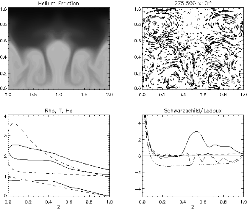
Figure 2: Simulation $I$. Same as figure 1 except at $t=2.755\%$ of a thermal diffusion time. The lower half of the domain is a well homogenized layer, as is seen in the helium concentration and mean field plots. The internal temperature transition layer is much thicker than the helium interfacial layer. The Schwarzschild/Ledoux criterion predict that the thermal boundary layer is unstable to oscillations but stable to convection. Weak oscillatory rolls are seen in the upper half domain in the velocity vector plot.

Three mechanisms contribute to mixing helium across the interface, the first being molecular diffusion enhanced by the sharp gradients there. From figure 2 it is also clear that there are significant regions where low helium concentration fluid is down-welled into the convection zone. Such regions are a remnant of both the original Rayleigh-Taylor plumes and the large amplitude interfacial waves which they excite. As time proceeds the lower layer becomes more well mixed, the interface sharpens and mixing by down-welling becomes less relevant. Finally, the scouring of the helium internal layer is a major source of vertical helium transport at all times.

The layer height is determined from $\bar{Y}$ by finding the height where $|\partial\ln\mu(\bar{Y})/\partial z|$ is maximum. Plotted in the first panel of figure 3 is the interface height as a function of time. After an initial growth phase, and except for internal wave oscillations, the layer height is seen to remain relatively constant with time. This implies that the sum of the interfacial mixing mechanisms do not contribute enough to destabilize the interface. Therefore the necessary condition for the formation of a second layer, a quasi-static interface, is satisfied.

Figure 3: Top: interface height as a function of time for simulation $I$. Bottom: Richardson number versus time. Until a layer is well developed, the Richardson number is not relevant, so we can disregard the high values of $Ri$ at early times.

The third mixing mechanism, internal layer entrainment, has the added effect of driving oscillations in the upper fluid in the following manner. As the interfacial wave rises, it drives an upward flow directly above the wave crest. Since the flow above the interface rises on hot plumes from below, this behavior is often referred to as the buoyancy coupling of two layers. When the wave turns downward, the flow in the upper domain continues upward and, through shear drag, is able to strip some of the helium rich fluid from the interface. Locally, fluid that has been stripped has greater helium concentration than its environment, yet due to its momentum it continues upward. Before being able to overturn completely, the density excess decelerates the flow and the roll turns around: this is the oscillatory instability of the upper fluid.

The helium rich, upward flowing fluid at $(x,z)=(1.0,0.75)$ in figure 2 is a product of this internal layer stripping. Plotted in figure 4 is the time trace of the vertical velocity field and $500$ times the helium deviation from its initial value at this point. The solid line clearly shows growing oscillations with period $\approx 1\%$ of a diffusion time and a longer growth time. The helium deviation is slightly out of phase with the velocity, which drives the oscillations. Parenthetically note that the ripples on the velocity trace clear at $t=2\%$ and elsewhere are due to sound waves.

Figure 4: Solid line: Vertical velocity field versus time in simulation $I$ at $(x,z)=(1.0,0.75)$. Dashed line: $500\times$ helium deviation at that point.

Though a layer has not yet fully developed by the end of the simulation $I$, one is obviously in the process of doing so. Since it contains both phenomena which are observed in laboratory layer formation, I conclude that it would likely form one if allowed to continue.

3.2 Simulation $II$: A vortex/shear layer.

Figure 5: Top: interface height as a function of time for simulation $II$. Bottom: Richardson number versus time.

The important differences of the second simulation are the lower aspect ratio, weaker forcing and initial conditions. For this run the initial velocity is set to a random spectrum of very low amplitude vortical waves with a wavenumber cut off at an intermediate length scale $(k_{max}\sim 20)$.

Again, the instability sets in through isolated, randomly spaced Rayleigh-Taylor plumes rising from the lower boundary. However, soon the flow becomes coherent and mixes the helium well in the lower half of the domain. At $t=0.07$ figure 5 shows that the interfacial layer height has saturated at $z=0.8$.

The flow in figure 6 is exceedingly elegant in its simplicity and merits some elaboration. The stable concentration jump is clear at $z=0.75$ in that $\epsilon_{L}<0$, while $\epsilon_{S}>0$ indicates that overstable oscillations should eventually set in. Moreover, an interfacial wave of the size of the domain propagates to the right. In the bulk of the well mixed region a strong shear layer has spontaneously arisen, reminiscent of the shear flow seen at high Rayleigh number Rayleigh-Bénard convection (though much less turbulent).

The shear at the bottom boundary aligns the flow so that heat fluxes into the fluid through one coherent thermal, located at $x\sim 0.8$ in the figure. Being carried by the shear, this thermal propagates leftward.

The entire shear layer is not stationary, rather it oscillates between closed flow lines and a single closed vortex, the eye of which is reforming at $(x,z)=(0.15,0.25)$. Merryfield (1995) produced a coherent structure in a weakly forced simulation, though in that case the vortex was a double gyre. In dynamical systems literature, an oscillating jet/vortex flow is referred to as separatrix reconnection, and takes place when a propagating wave is modulated at another frequency. In this case, the second period is provided by the leftward propagating thermal at the base of the flow which interacts with the rightward propagating interfacial wave above.

Figure 6: A thick layer with sharp density jump is clear seen in both the $Y$ concentration and Ledoux Criterion in simulation $II$. The strong strong shear layer and traveling coherent vortex form spontaneously and are long lived. Helium transport is enhanced by separatrix reconnection as is in the low helium at the trough of the interfacial wave in the upper left panel.

Jets of collimated flow, like the one below the interface in figure $3.6$ are notoriously stable to advective transport across them, and one would expect molecular diffusivity to be the primary mode of helium mixing across the interface. However, separatrix reconnection provides a mixing channel so that, even in this simple flow, it is able to entrain helium poor fluid through the trough of the interfacial wave (particularly evident in the plot of helium fraction).

Finally, take note of the small knee in the temperature average and the corresponding peak in $\epsilon_{S},\epsilon_{L}$. This is the imprint of the coherent thermal which, owing to the vortex and shear, mixes with the rest of the flow through discreet release events.

Though performed at high Prandtl number, this simulation holds an important lesson for astrophysical layering. Even in a weakly forced scenario where the interfacial waves are very low amplitude, mixing by separatrix reconnection will provide much greater cross interface helium transport than molecular diffusion enhanced by the sharp gradient there.

3.3 Low Prandtl Number

3.3.1 Simulations $III$: No layering

Simulations $IIIa,b$ are presented as two cases in which, according to the analytic theory described in §5.1, interfaces should form. In both cases layered convection does not occur, but for different reasons.

In $IIIa$ the stabilizing compositional gradient is not sufficient to impede the rising Rayleigh-Taylor plumes. Consequently, they hit the top boundary before turning back and eventually coalescing. By $t=0.061$ in figure 7 the helium is already well mixed and the convection is global.

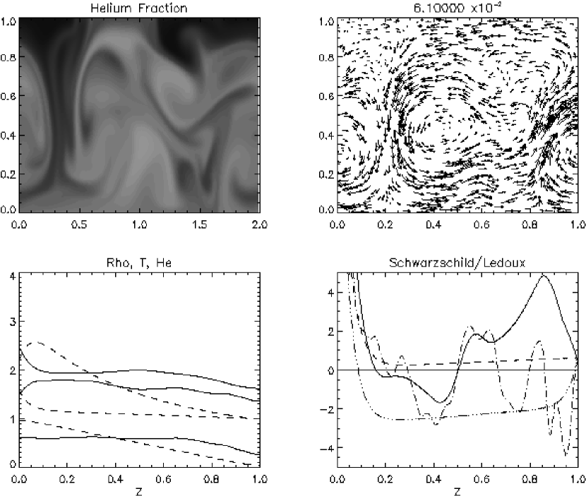
Figure 7: At $t=0.061$ the convection in $IIIa$ has effectively mixed the whole fluid.

A relation for the quasi-static interfacial layer height in terms of the heat flux, the initial buoyancy frequency of the domain and empirically determined factors was given by Fernando (1989) and will be discussed at length below. Suffice for the moment to say that the critical height varies as the square root of the heat flux at the lower boundary and is thus proportional to $\sqrt{Ra_{T}}$ there. Guided by this and the previous failure, a heat flux one fifth that of $IIIa$ is chosen, with the expectation that a layer should saturate within the height of the domain. However, by $t=0.07$ in $IIIb$ the lower thermal boundary layer has diffused to $z=0.5$ though convection has yet to set in. Correspondingly, the whole region $z<0.5$ has become Ledoux unstable. It is reasonable to conclude that the growth rate of the plumes is too low to observe convection before the Ledoux unstable region encompasses the entire computational domain. Global convection would thus ensue.

This is an interesting result, but probably less relevant for astrophysics on two counts. First, astrophysically high Rayleigh numbers yield correspondingly large growth rates. Second, the simulation was initialized with a small velocity field; more realistic in nature would be a spectrum of finite amplitude gravity waves, allowing to avoid the, somewhat long, linear growth phase.

3.3.2 Simulations $IV$, $V$, $VI$: Layer formation and interface migration

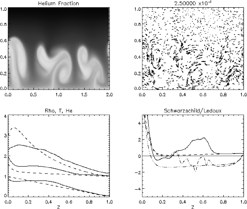
Figure 8: At $t=0.025$ in simulation $IV$ the plumes have mostly stopped at the midplane through a combination of buoyancy contrast and enhanced drag. Parts of the plumes which remain buoyant continue upward.

Stars have both small Prandtl number and exceedingly large Rayleigh numbers and, to the limit of computational feasibility, these conditions are reproduced in simulations $IV,\,\,V$ and $VI$.

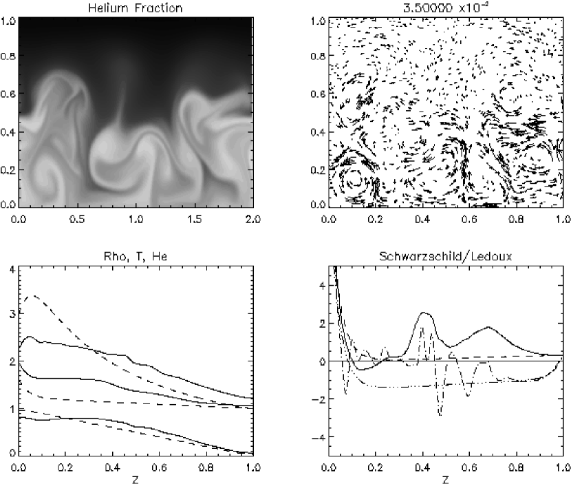
Figure 9: At $t=0.035$ in $IV$ the plumes have overshot their equilibrium height and fall. A lower layer, clearly evident in the horizontal mean fields, begins to form. The thin helium rich filament above the mixing region has been stripped from a plume which overshot.

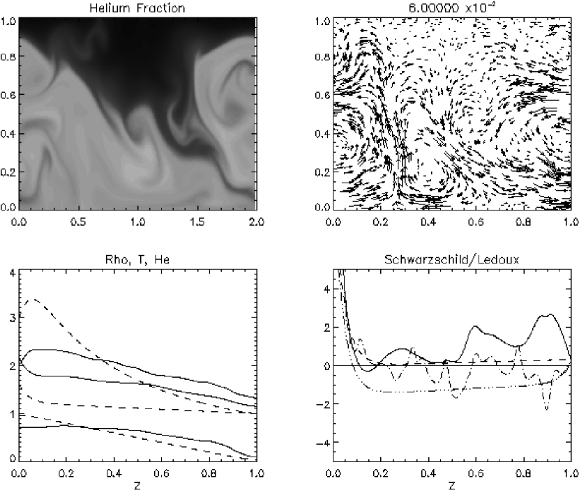
Figure 10: Though the flow is highly disordered in $IV$, a large internal wave dominates the mixing through down-welling. The mean fields and $\epsilon$ give no hint of the highly distorted interface.

Figure 11: Interface height and Richardson number for $IV$.

Figures 8 - 10 are the $t=0.025,$ $0.035$ and $0.06$ snapshots of simulation $IV$ in which a small initial velocity spectrum is used to seed the Rayleigh-Taylor instability. By $t=0.025$ the plumes have reached $z=0.5$ and slowed significantly. Notice, though, that smaller plumes with a large helium contrast are still able to rise from the interface of the main plumes; this plume splitting is seen at the center of the $Y$ concentration plot. Though mostly having stopped near the midplane the plumes are still slightly buoyant, therefore the primary mechanism slowing them must be their drag.

Even though viscosity is weak, it is well known that drag can be significantly enhanced by the adiabatic expansion of rising plumes, the entrainment of fluid into the plumes and the breakup of the plume tip. Since it is clear that parts of the plumes remain buoyant after breakup and continue to penetrate up to $z=0.7$ then, necessarily, buoyancy and thermal diffusion out of the plumes play a smaller role in their deceleration up to the midplane.

In figure 9 the plumes have turned around and begin to resemble convecting cells mixing the bottom half of the domain. However, during the deep penetration, there is significant mixing of helium rich fluid up to $z=0.8$, the shadow of which are the faint plumes seen in the upper half plane. Like the scoured interfacial layer in simulation $I$, these faint plumes have a $Y$ greater than their surroundings and can be expected to descend. Also like their counterparts, these plumes are in a region which is apparently oscillatorily unstable. However, a clear interface has yet to form above the convecting region and no oscillatory instability is apparent for $z>0.5$ at $t=0.035$.

From interface formation to $t=0.06$ in figure 10 the flow becomes turbulent, but with a persistent large scale component. In turn, these few large vortices and plumes drive an interfacial wave of wavelength approximately equal to the domain length. At this point $\epsilon_{L}$, $\epsilon_{S}$ are irrelevant measures of convective stability as the interface is clearly not horizontal. Unlike the high Prandtl number case, this interfacial wave is of very large amplitude and all of the mixing mechanisms thus far discussed take place across it. Needless to say, molecular diffusion enhanced by the interfacial gradient plays a relatively small role in the total transport.

Most obvious from figure 10 is the strong down-well obliquely crossing the domain and upon which a helium rich internal wave is about to break. This is a more dramatic version of the separatrix reconnection demonstrated in $II$. Traces of previous mixing events are seen as helium poor filaments in the otherwise mixed region. Less obviously, the upper left of the thick helium boundary layer is experiencing scouring by a flow along the interface (around $(x,z)=(0.5,0.9)$). Moreover, a down-flow near the mouth of the down-well (at the center of the domain) is clearly shearing two helium lamina, though where they will mix is not clear. Irrespective, this flow is violently mixing the domain and by $t=0.07$ the interfacial wave collides with the upper boundary so that no second layer can be formed.

Interface height is plotted against time in figure 11. Except for the last fraction of a diffusion time ($\sim 10^{-3}$), the interface compares well with that of figure 3. The spikes betray the large amplitude internal waves on the interface and the collapse of the interface near the end reflects the overturning convection which sets in at that time.

Figure 12: Temperature plot of $VI$ at the $t=0.03$ showing isolated thermals emanating from the bottom boundary. In the helium field (not shown) the plumes have begun to form an interface at this time.

Each of the dynamic mixing mechanisms have at their source the fact that the amplitude of the interfacial wave is very large, comparable to its wavelength. This, in turn, may be a consequence of both the fact that the flow under consideration is 2-dimensional and that the aspect ratio of the domain is small, $\lambda=2$. In 3-d simulations this inverse cascade would not occur while, since rolls will not likely have wide aspect ratio themselves, it would be irrelevant for large aspect ratio 2-d boxes.

In simulation $VI$ an attempt is made to study the effect of large aspect ratio on, in particular, the amplitude of the interfacial wave. Unfortunately, the simulation lost resolution and had to be ended before an interface was well developed. Nonetheless it is evident from the temperature field shown in figure 12 that rising thermals are well spaced along the bottom boundary and there is some hope that, should many weak thermals persist, the flow would not produce such large scale structures particularly, the catastrophic internal wave.

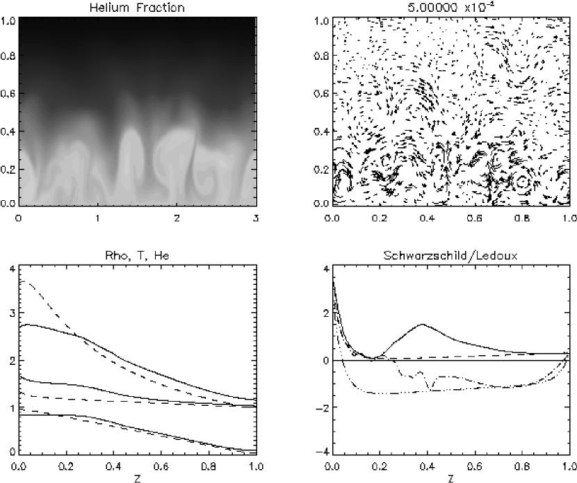
Figure 13: After $t=0.05$ in simulation $V$ a sharp layer has formed below $z=0.35$, where the convection is less vigorous than in previous simulations. Nontheless, the convection generates narrow structures which account for most of the mixing with the static fluid above.

The most promising case for layer formation is provided by simulation $V$. Akin to $IV$, it has lower heat flux at the bottom boundary and larger aspect ration ($\lambda=3$), the objective being that the layer height should saturate at smaller $z$ and that the convection should not be dominated by large structures. Figure 13 shows that this is indeed the case since by $t=0.05$ the interface has reached a quasistationary height of $z=0.35$. Notice that the time is much later than in previous simulations since the flow is much weaker. The thermodynamic criteria are favorable to onset of oscillations just above the interface and already at this early time such oscillations are seen in the fluid above. Despite weak convection in the lower layer, the interface in figure 13 is strikingly irregular. Though the interfacial waves remain small, mixing is again dominated by large structures being engulfed between the plumes below the interface.

By $t=0.096$ the interface has continued to migrate upward, and the density jump is below $z=0.6$ in figure 14. Interfacial scouring due to oscillatory convection in the upper fluid creates filaments of helium rich fluid above the interface and mixing below remains dominated by large blobs of fluid between the plumes.

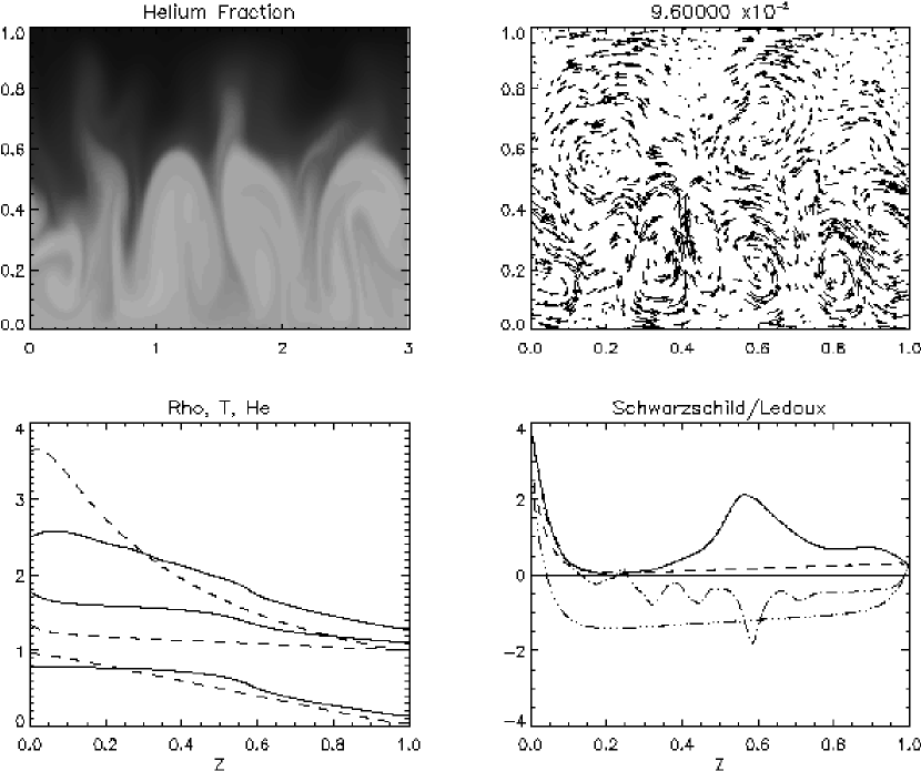
Figure 14: At $t=0.096$ the layer has migrated to $z\sim 0.5$ and interfacial waves are quite large. Entrainment at wave crests continues to be the main source of mixing. By now, weak oscillatory convection is taking place in the upper half of the fluid and causing helium to be scoured upward from the layer interface.

Large plumes have penetrated to $z=0.8$ by $t=0.136$ (figure 15) effectively destroying the oscillatory flow which had been growing there. Two plumes dominate the flow at this time and are clearly able to entrain large, helium poor fluid elements downward into the convection as is seen at $(0.6,0.3)$ in the figure. Interfacial splashing, evident in a thin filament above this blob, overtakes scouring as the principal mechanism for helium transport above the interface.

Though the vestiges of a layer are evident in the mean helium field, the interfacial waves have grown large enough to nearly reach the top boundary, suggesting that a second layer will not form before the interface grows to encompass the whole fluid. Such waves, though less marked, are clear in figure 16. Nonetheless, this is the only case discussed thus far where the theoretical prediction of Fernando (1989), $h\sim\sqrt{t}$, provides an excellent fit. The curve $h=1.8\sqrt{t}$ agrees well with the data after $t=0.01$ and despite the growing interfacial waves at late times. Furthermore this fit yields an effective diffusion coefficient across the interface of $\tau_{eff}=1.62$: it will be shown subsequently that this greatly exceeds the mixing provided in existing models.

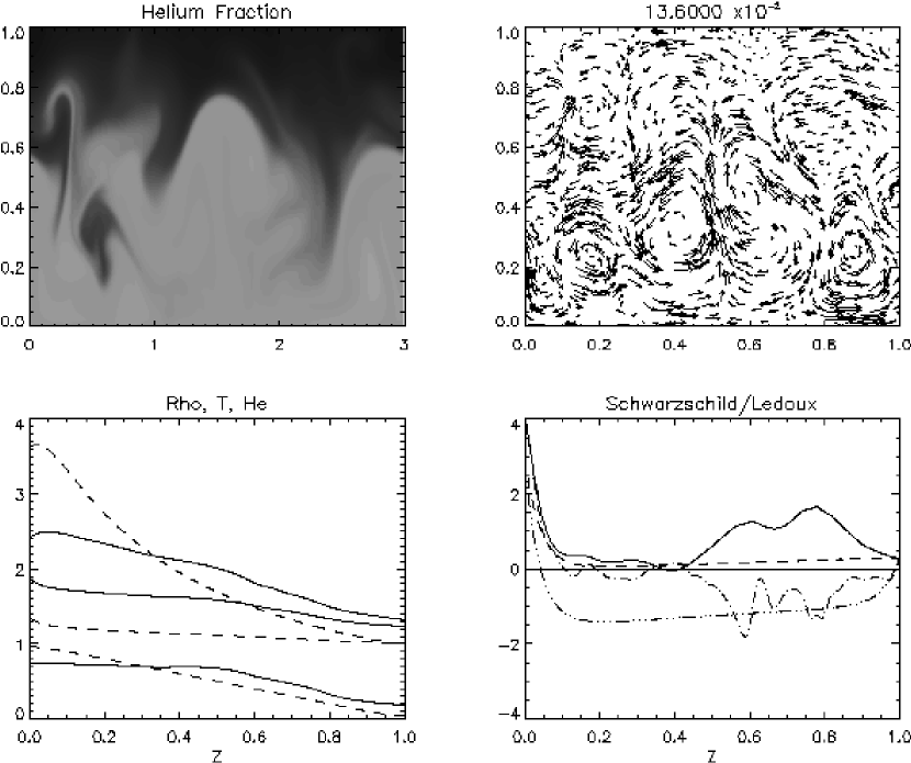
Figure 15: At the end of $V$, at $t=0.0136$ a large blob of helium poor fluid is being entrained into the lower layer. Though the thermodynamic criteria remain favorable for a second layer to form and there persists a helium gradient in the top $z=0.4$ of the domain, it seems unlikely that oscillatory convection will be able to overcome the entrainment from the interface.

Even in this most weakly forced example where the aspect ratio of the convecting fluid remains greater than $6$ for most of the simulation, there persists an inverse cascade to large scale structures. Figure 17 shows a space time plot of the temperature perturbation on the bottom boundary. Hot spots, or thermals, along this boundary are seen as bright filaments in this plot; from here plumes rise and convection is driven. It is clear that the main plume dynamic is one of coalescence for, even though approximately $10$ thermals arise at the onset of convection, only two large thermals are apparent by the end. Furthermore, weak plumes are continually formed and incorporated into the stronger ones since the convection tends to direct flow toward strong plumes on the boundary. Two plumes implies four large scale rolls and since at $t=0.136$, $h\sim 0.7$ the aspect ratio of each roll is $\sim 1.1$, less than, but not atypical of large structure in regular Rayleigh-Benard convection. One must therefore conclude that the aspect ratio of layered convection will remain $\approx 1$ irrespective of the layer height.

Figure 16: Layer height and Richardson number versus time for $V$. A fit of $h=1.8\sqrt{t}\,\,$ is included and yields a effective diffusion coefficient of $\approx 1.62$ (see figure 23).

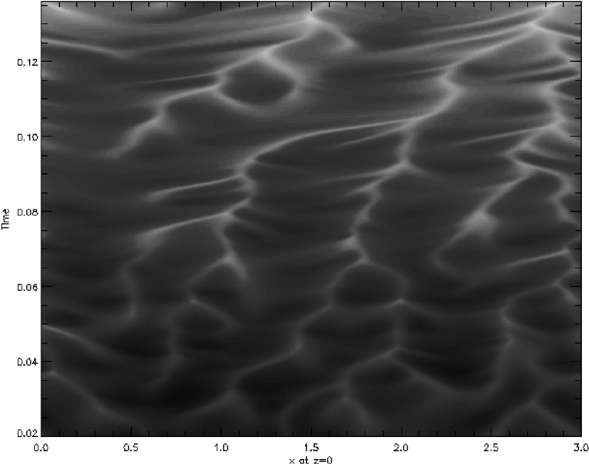
Figure 17: Space-time plot of temperature perturbation evaluated along the bottom boundary in simulation $V$. There are clearly several hotspots at early times which eventually coalesce and become plumes. By the end (top of the figure) only two, very strong plumes remain.

Therefore, as to the the question of whether a second layer forms, the results for low Prandtl number are inconclusive but not promising. Since the large amplitude internal wave seen in $IV$ and $V$ drive instabilities along the interface and are a source for much cross interface mixing it remains possible that any layer can continually entrain fluid from above before oscillatory convection becomes well developed. Whether this is simply due to the strong forcing or to the relatively small aspect ratio under consideration remains to be clarified. If due to the latter, then it can be argued that in a stellar context where aspect ratios are large, such a large interfacial wave will not exist.

If, in fact, the fluid is forced too strongly in $IV$ and $V$ then there still remain several possibilities. It is clear that the convection continues to inverse cascade to larger scales at each stage, so that plumes within a layer are always spaced at a distance about twice the layer height. The plumes generate the interfacial waves reaching amplitudes of significant fractions of the layer thickness (particularly clear in figure 15) which may persist, constantly entraining fluid from above in broad down-flows. In such a circumstance an oscillatory instability would be unable to set in above the interface and eventually a state of global, classical convection would exist.

On the other hand, the interface may continue to migrate upward, gradually stabilizing until the plumes flatten along the buoyancy jump at the interface and are no longer able to excite large waves there. This mechanism occurs in the laboratory and is the motivation for introducing the Richardson number (equation 3). A low value of $Ri$ implies that the interface should migrate upward and Fernando (1989) measured a critical value for this behavior in the laboratory. The bottom panels in figures 3, $3.5$, 11 and 16 trace the interfacial Richardson number with time for simulations $I$, $II$, $IV$ and $V$, respectively. That $Ri$ is smallest in case $IV$ is consistent with the observed layer migration; in fact, in case $IV$ it is just within the range of the critical number measured in the laboratory experiments of Fernando (1989) where $Ri_{crit}\sim 2-30$.

Throughout simulation $V$, however, the Richardson number is greater than $\sim 50$, well above the critical value measured by Fernando (1989). However, the interface continually migrates upward and interfacial waves increase with time, as opposed to decreasing. Compare this with simulation $I$ (figure 3) where $Ri<50$ for a short period of time yet the interface does not migrate appreciably. Such observations can be most readily explained if the interfacial Richardson number at late times is below the critical value and thus provide strong evidence that the critical interfacial Richardson number should increase with decreasing Prandtl number.

4 Low Prandtl Number Convection Impinging on a Stable Compositional Interface.

In order to isolate the mixing experienced at a stable interface from the question of the formation of that interface, simulation $VII$ is initialized with $Y=0$ in the top half of the domain, $Y=1$ in the bottom and a thin ($\sim.05$) transition region between.

By $t=0.014$, (figure 18) the convection has set in throughout the lower layer. Though the density jump still stabilizes the interface, waves are apparent. Again, mixing takes place at the troughs of these waves and in the helium plot there are two significant helium rich structures penetrating into the upper layer. Some interfacial scouring has occured, but is apparently much weaker than the wave breaking. Although $\epsilon_{S}>0$ just above the interface, there is yet no motion in the upper layer beyond its interaction with the interfacial wave.

Figure 18: Convection has set in throughout the lower layer by $t=0.014$ in simulation $VII$. Interfacial waves are still small, but on breaking they mix significant amounts of helium into the upper layer. Scouring is apparent just above the interface at $x=1.8$.

By $t=.027$ the interfacial wave breaking is very significant and a large mixing plume is seen in figure 19. The concentration jump has barely been eroded and the interfacial wave is still of moderate height ($\sim 0.07$) yet its self interaction is able to generate large structures, much like the interaction of two solitary waves on the surface of water.

In the upper half of the domain, not only is flow visible around the helium plume, but also ahead of it, resembling the upstream field of a weak vortex (notice the velocity in 19). This weak vortical flow, however, is unable to fully develop into convection before it becomes disrupted by the interfacial wave below. Clearly in figure 20 the flow in the upper half plane is soon dominated by the interfacial wave, which by $t=0.042$ has grown quite large.

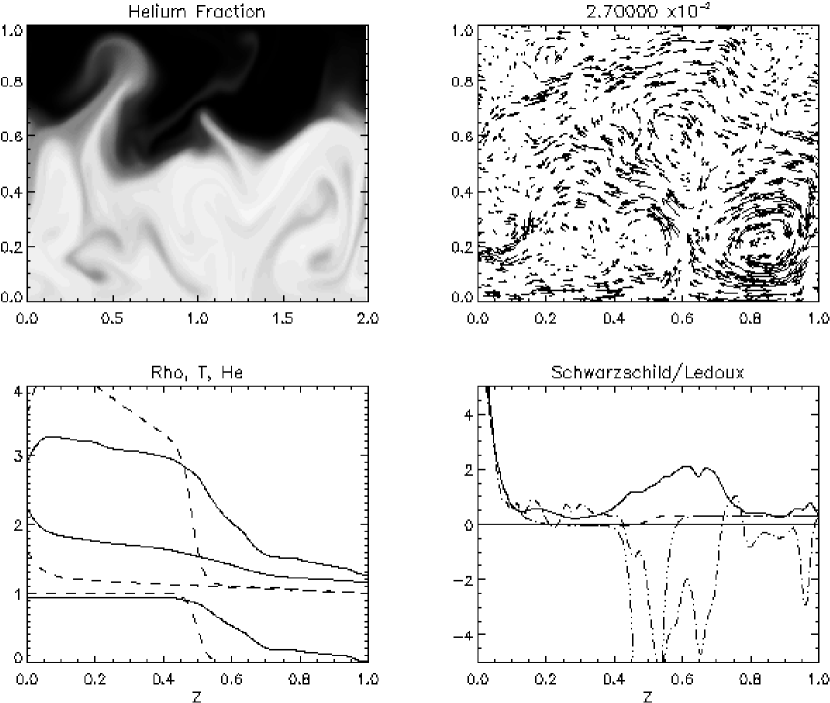
Figure 19: A large helium plume results from the self interaction of relatively small interfacial waves. The interface is still very stable.

Though this simulation deals with an idealized setting, it is obvious that the structures in the flow are less simple. In particular, the distinction between “helium mixing plume”, which results from the interaction of two gravity waves, and a large amplitude gravity wave is not precise. Gravity waves below an interface are also referred to as penetrative convection and have been studied numerically (see Massaguer et al. (1984), Hurlburt et al. (1994)) and analytically (Schmitt et al. (1984), in the context of a fixed stability interface). The current results are complicated by the fact that the stable interface itself interacts with the flow, yielding a highly nonlinear wave pattern and blurring previous distinctions of plume and wave. The structure in figure 19 is classified as mixing because, for the most part, it becomes entrained in the uppper fluid. The large interfacial wave in figure 20 is described as such because, although there is significant scouring of its upper boundary and entrainment at its crest, it mostly returns to the lower layer intact.

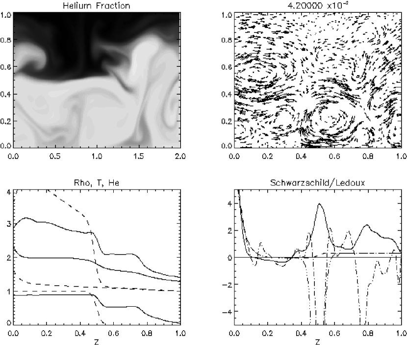
Figure 20: Motion in the upper fluid is relatively insignificant still by $t=0.042$. A plume driven interfacial wave dominates the figure and is seen as a second knee ahead of the interface in the mean field plots. $\epsilon_{L}\ll 0$ implying that the interface remains stable.

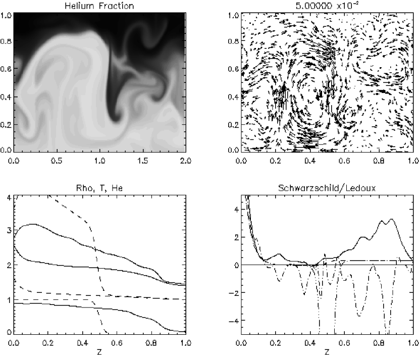
Figure 21: The up-flow is dominated by a single thermal on the bottom boundary which excites a very large amplitude, large scale interfacial wave. Though an interface is barely apparent in the mean field plotes, it is clear from the helium concentration that the fluid is not well yet mixed.

Using the Richardson number as a criterion for buoyancy stability, one concludes that the interface is stable throughout the simulation This is in stark contrast to the fact that interfacial waves are significant and at $t=0.05$, figure 21, are of amplitude equal to the layer height. As in the prior simulation, this discrepancy results from the fact that at late times the up-flow at the lower boundary concentrates into one dominant rising thermal. Recall that the Richardson number, plotted in figure 22 for this case, is the ratio of the buoyancy across an eddy height to the average kinetic energy in the lower layer: a mean field argument. Since the buoyancy and resulting momentum of the thermal plume is much greater than would be anticipated from a mean field argument it is able to penetrate much deeper than expected.

From figure 22 the conclusion should be drawn that, since the average kinetic energy in the lower domain is always $>1/40$ the potential energy wall of the interface, convection should not penetrate deeply. However, it is obvious from figure 21 that the flow is collimated in the strong thermal up-flows, thus the average kinetic energy is not a good representation of the dynamics in the lower layer.

Therefore it is also clear from this simulation that if the lower layer develops a large scale convective roll, then the interfacial wave will have a large scale and correspondingly large amplitude. Furthermore, figure 21 dramatically shows that in such instance, mixing is dominated by entrainment below the wave trough and by scouring of the interface from above through the weaker flow generated by the interfacial wave above it.

Figure 22: The interface height and Richardson number in the two layer simulation, $VII$.

5 Discussion

5.1 Comparison with previous work

Figure 23: Solid line is the calculated diffusion coefficient from a $h\propto t^{1/2}$ fit of $V$. Asterisks are calculated from Stevenson (1979) while triangles are calculated from Spruit (1992); time averages of the latter two are added.

Figure 24: The stability parameter for the interface of $VII$ derived using predictions from Stevenson (1979) - solid, Fernando (1989) - dash and Spruit (1992)- dot-dash.

I remind the reader of the mixing theories of Stevenson (1979), Spruit (1992) and Fernando (1989), in order to compare them with these simulations. The former two provide mixing length theories of semiconvection in the presence of layers and, therefore, effective diffusion coefficients for transport across these layers. The latter derives the equilibrium height of the first layer through energy arguments and provides a criterion for onset of convection above the first layer.

First let us consider Fernando (1989). Using conservation of energy and molecular weight and with the assumption that the kinetic energy available to convection is proportional to the heat flux from the boundary, he derived the following relation

$$h_{c}\approx C\left[\frac{Ra_{T,\,bot}}{Ra_{He}^{\frac{3}{4}}Pr^{\frac{1}{2}}}\right]^{\frac{1}{2}}$$ (17)

for $h_{c}$, the critical interface height of the first layer. The constant, $C$ must be determined experimentally as it contains the parameters of convective efficiency and its dependence on $Pr$ is not at all known. Calibrating the numerical experiments to the theory may not be reasonable, but the theory can be used to compare the simulation results amongst themselves. By calibrating the constant to simulation $II$, where $h_{c}=0.8$, equation (17) yields the critical layer heights $h_{c}=0.50,\,\,1.4,\,\,0.63,\,\,1.0,\,\,0.55$ for simulations $I,\,III(a),\,III(b),\,IV$ and $V$ respectively. Though not quantitatively correct, these agree qualitatively with the observation of a layer in $I$ and $V$, plumes impinging on the upper boundary in $III(a)$ and interfacial waves hitting the upper boundary in $IV$. The lack of layering in $III(b)$ cannot, of course, be explained by this theory.

Of the necessary criteria suggested at the outset for the formation of a second layer, only simulation $I$ satisfied them both. Since it would be useful to refine them, we must now turn our consideration to the dynamics of the interface above the layer. Fernando (1989) reproduced the observation of Turner (1968) that the onset of a second layer requires the Rayleigh number in the interfacial region be sub-critical to overturning convection. If the interfacial thickness is denoted $\delta$ then this amounts to the requirement that $\delta\ll h_{c}$. Again, using energetic arguments, it can be shown that

$$\frac{\delta}{h_{c}}=\frac{Ra_{crit}^{\frac{1}{4}}}{\sqrt{2}C}\left[\frac{Ra_{T}Pr}{Ra_{He}}\right]^{\frac{1}{4}}$$ (18)

where the Rayleigh numbers are to be measured at the interface level and $C$ is the same as in equation (17). The critical Rayleigh number, $Ra_{crit}$ must also be determined experimentally and was found to be rather higher than that of classical convection, making the combination of constants of order one.

This can be reworked into necessary condition for the onset of oscillatory convection above the first layer and, amounts to

$$\Sigma_{Fern}\equiv\frac{\epsilon_{S}}{\nabla_{\mu}}\ll\frac{4C^{4}}{Ra_{crit}Pr}.$$ (19)

Again experimental results suggest that the combination of constants on the right hand side are order one.

The theories of Spruit (1992) and Stevenson (1979) give effective diffusion coefficients for helium transport across an interface under the respective assumptions of enhanced diffusion or internal wave breaking. If the rate of diffusion is greater than the growth rate of oscillations above the interface, then the region above will slowly be entrained into the convection below. Otherwise, there is some hope for the growth of oscillations above. The growth rate of weakly forced overstable modes of wavenumber, $k$, is

$$\gamma=\frac{\epsilon_{S}}{2|\epsilon_{L}|}k^{2}$$ (20)

while the effective molecular diffusivities are

$$\tau_{wave}=\left[\frac{\epsilon_{S}}{\nabla_{\mu}}\right]^{2}$$ (21)

and

$$\tau_{diff}=\sqrt{\tau}\frac{\epsilon_{S}}{\nabla_{\mu}}$$ (22)

for Stevenson’s wave model and Spruit’s enhanced diffusion model, respectively. The rate of diffusion of modes $k$ is proportional $k^{2}\tau_{eff}$ and the requirement that oscillations grow more rapidly than a diffusion time yields the stability criteria

$$\Sigma_{wave}\equiv\frac{\epsilon_{S}}{\nabla_{\mu}}\frac{|\epsilon_{L}|}{\nabla_{\mu}}\ll 1$$ (23)

and

$$\Sigma_{diff}\equiv\sqrt{\tau}\frac{|\epsilon_{L}|}{\nabla_{\mu}}\ll 1$$ (24)

respectively for the two theories.

The effective diffusion coefficients and stability parameter predicted by each theory can be measured by evaluating $\epsilon_{S}$ and $\nabla_{\mu}$ at the interface. Figure 23 compares $\tau_{wave}$ and $\tau_{diff}$ with the fit $h=1.8\sqrt{t}$ to simulation $V$ which yields $\tau_{eff}\approx 1.62$. While the difference of both theories with the numerical data is astonishing, the enhanced diffusion model further suffers from the fact that it is proportional to $\sqrt{\tau}$, a negligibly small number in stars.

The variation of the stability criteria with time for simulation $VII$ is plotted in figure 24 and they all notably remain less than one, but not significantly so. Again, the criterion $\Sigma_{diff}$ is proportional to $\sqrt{\tau}\,(\sim 1/3$ here) meaning that, in the limit of small molecular diffusivities, layered convection will always occur. This conclusion simply results from the assumption that only enhanced diffusive transport acts across the interfaces, inconsistent with the wave breaking seen in the simulations.

Both $\Sigma_{Fern}$ and $\Sigma_{wave}$ were derived considering buoyancy effects, yet the fact that they agree well throughout most of the simulation is still striking. This agreement results from the fact that the Ledoux criterion is dominated by the compositional gradient at the interface, $|\epsilon_{L}|\sim\nabla_{\mu}$. Nonetheless, it is clear that $\tau_{wave}$ underestimates the true layer entrainment and thus the stability criterion is overestimating the stability of the layer. Therefore, it seems unlikely that a second convecting region will form above the interface in $VII$ even though the Richardson number criteria indicates that it should be stable.

5.2 Conclusions and future work

These simulations have reproduced layer formation in the context of laboratory flows and distinguish the mechanisms for transport across a compositional interface: enhanced diffusion, scouring and wave breaking. They also confirm the difficulty of forming layers in a low Prandtl number fluid. Characteristic of all of the results is the inverse cascade of velocity to large length scales resulting in strong isolated upward rising thermals which are able to excite high amplitude, long wavelength waves on the interface. Mixing across the interface is dominated by wave breaking in all of the low Prandtl number cases; even, and most importantly, when the interface is prescribed and highly stable ($VII$).

Though it remains to be determined whether strong, isolated thermals develop in a three dimensional fluid, it can yet be safely concluded that, at low Prandtl number, cross interfacial mixing will be dominated by wave breaking. This is especially evident at early times in $VII$ where even small interfacial waves drive large “splashes”, mixing helium high into the stable layer. Therefore, the criteria associated with the Stevenson (1979) or Fernando (1989) theories of interfacial mixing seem to be the most appropriate for determining whether a second layer, and thus multiple layers, will form. Even so, these theories greatly underestimate the mixing across the interface.

This underestimate is linked to the the large interfacial waves and therefore the critical Richardson number for the stability of an interface. Comparing simulation $V$ to the low Prandtl number case, $I$, it is clear that the critical Richardson number must increase with decreasing Prandtl number.

Further study of whether the estimate of Stevenson (1979) truly underestimates mixing requires determining whether or not the large interfacial waves persist in 3-dimensional simulations and at large aspect ratio. Though the former would be most valuable, a parameter space study is not computationally feasible. The best prospects for sorting out the issue of isolated thermals rests in continuing this work at larger aspect ratios.

The simulations I have presented envision a scenario where an energy flux is abruptly turned on below a region which is marginally unstable to semiconvection. This results in the formation of layered convection due to the redistribution of a compositional gradient in a thin layer and on time scales short compared to a thermal diffusion time. The convection within such a layer is concentrated in plumes spaced such that the largest rolls have aspect ratio approximately $1$. The interface itself is characterized by large internal waves and smaller breaking waves, making it ineffective as a barrier to transport. Since, in all cases considered, the fluid is very well mixed after a small fraction of a thermal diffusion time, it is unlikely that layering caused by buoyancy disruption would play any role in stellar convection. In fact, the very large effective diffusion measured herein suggests that such layered structures are so unstable as to make them dynamically unimportant even when a compositional gradient is redistributed by other mechanisms such as rotation or large internal waves, which set up initial conditions similar to $VII$.

References

- Balmforth & Biello (1998) Balmforth, N.J. & J. A. Biello 1998 Double diffusive instability in a tall thin slot. J. Fluid Mech. 375 203-233.
- Balmforth et al. (1998) Balmforth, N.J., S. G. Llewellyn Smith & W. R. Young 1998 J. Fluid Mech. 355 329-358.
- Biello (1997) Biello, J. A. 1997 Aspects of double diffusion in a thin vertical slot. In Double Diffusive Processes, 1996 Summer Study Programme in Geophysical Fluid Dynamics, Woods Hole Oceanog. Inst. Tech. Rep. WHOI-97-10.
- Bruenn & Dinhva (1996) Bruenn, S. W. & T. Dinhva 1996 The role of doubly diffusive instabilities in the core-collapse supernova mechanism. Astrophys. J. 458 L71-L74.
- (5) Canuto, C., M. Y. Hussaini, A. Quarteroni, T. A. Zang, 1988 Spectral Methods in Fluid Dynamics, Springer Verlag.
- Canuto (1999) Canuto, V. M. 1999 Turbulence in stars. III. Unified treatment of diffusion, convection, semiconvection, salt fingers, and differential rotation. Astrophys. J. 524 311-340.
- Canuto (2000) Canuto, V. M. 2000 Semiconvection and overshooting: Schwarzschild and Ledoux criteria revisited. Astrophys. J. 534 L113-L115.
- Cortesi et al. (1999) Cortesi, A.B., B.L. Smith, G. Yadigaroglu & S. Banerjee 1999 Numerical investigation of the entrainment and mixing processes in neutral and stably-stratified mixing layers. Phys. Fluids 11 162-185.