An analytic function fit to Monte-Carlo X- and $\gamma$-ray spectra from Thomson thick thermal/nonthermal hybrid plasmas

Abstract

We suggest a simple fitting formula to represent Comptonized X- and $\gamma$-ray spectra from a hot ($kT_{e}\gtrsim 10$ keV), Thomson thick ($\tau_{T}\gtrsim 5$) hybrid thermal/nonthermal plasma in spherical geometry with homogeneous soft-photon injection throughout the Comptonizing region. We have used this formula to fit a large data base of Monte-Carlo generated photon spectra, and provide correlations between the physical parameters of the plasma and the fit parameters of our analytic fit function. These allow us to construct Thomson thick Comptonization spectra without performing computer intensive Monte Carlo simulations of the high-$\tau_{\rm T}$ hybrid-plasma Comptonization problem. Our formulae can easily be used in data analysis packages such as XSPEC, thus rendering rapid $\chi^{2}$ fitting of such spectra to real data feasible.

Accepted for publication in The Astrophysical Journal Supplement Series

1 Introduction

Compton upscattering of soft (optical, UV or soft X-ray) radiation by hot ($kT_{e}\gtrsim 10$ keV) plasma is believed to play an important role in the formation of high-energy (hard X-ray and $\gamma$-ray) spectra of many astrophysical objects. Some examples are Galactic X-ray binaries (for recent reviews see Tanaka & Lewin (1995); Liang (1998)), supernova remnants (e.g., Hillas et al. (1998); Aharonian (1999)), Seyfert galaxies (for recent reviews see Mushotzky et al. (1993); Zdziarski (1999)), blazars (Maraschi et al. (1992); Dermer et al. (1992)), the intergalactic medium (Sunyaev & Zeldovich (1980); Rephaeli (1995)), and possibly also $\gamma$-ray bursts (Liang (1997); Liang et al. (1999)).

Comptonization in purely thermal plasmas is fairly well understood, and analytical solutions for the emerging hard X-ray and $\gamma$-ray spectra for a wide range of Thomson depths and plasma temperatures have been developed (Sunyaev & Titarchuk (1980); Titarchuk (1994); Titarchuk & Ljubarskij (1995); Hua & Titarchuk (1995)). However, the currently known solutions can not be applied to hybrid thermal/nonthermal or even purely nonthermal plasmas, which are believed to be the primary source of hard X-ray radiation in many astrophysical objects. For example, Li, Kusunose, & Liang (1996) have shown that the high-energy spectrum of Cyg X-1 can be plausibly reproduced by Comptonization in a quasi-thermal plasma with a small fraction of electrons in a nonthermal tail. Thermal/nonthermal hybrid models have also been discussed in the context of the high-energy spectra of Seyfert galaxies, e.g. NGC 4151 (Zdziarski et al. (1994); Zdziarski, Johnson, & Magdziarz (1996)). The development of such nonthermal tails has been confirmed by Böttcher & Liang (2001) by detailed Monte-Carlo/Fokker-Planck simulations of radiation transport and electron dynamics in magnetized hot plasmas, e.g. in accretion flows onto compact objects.

We need to point out that the combination of soft- to medium-energy X-ray spectra (typically integrated over a few ksec) with hard X-ray / soft $\gamma$-ray OSSE spectra (typically integrated over hundreds of ksec or even several days) could introduce artificial spectral signatures due to the superposition of thermal Comptonization spectra from different emission regions, possibly at different times. However, the detailed Fokker-Planck simulations of the dynamics of electron acceleration and cooling in coronal plasmas in the vicinity of accreting compact objects (e.g., Li et al. (1996); Böttcher & Liang (2001)) clearly demonstrate that nonthermal tails in the electron distributions are very likely to be produced in such environments. It is thus desirable to have simple, analytical expressions for the Comptonization spectra arising in this case.

For the general case of arbitrary Thomson depth, average electron energy (i.e. temperature), nonthermal fraction of electrons in the hybrid plasma, and nonthermal electron spectral parameters, the most reliable and often fastest method for computing Comptonization spectra is the Monte-Carlo method (Pozdnyakov et al. (1983)). However, Monte-Carlo simulations of Comptonization problems become extremely time consuming in the case of very high Thomson depth, $\tau_{\rm T}$, since the number of scatterings that need to be simulated, increases $\propto\tau_{\rm T}^{2}$. To date, there are no simple, analytic approximations to the problem of optically thick Comptonization in hot, thermal/nonthermal hybrid plasmas. This has made $\chi^{2}$ minimization fitting of such models to real data infeasible until now.

Using our linear Monte-Carlo Comptonization codes, we have built up a data base of over 300 Comptonization spectra from hot, Thomson thick, thermal/nonthermal hybrid plasmas with different Thomson depths, temperatures, nonthermal electron fractions, spectral indices and maximum electron energies of nonthermal electrons. In this paper, we propose a simple analytic representation, consisting of an exponentially cut-off power-law plus a smoothly connected double-power-law (Band et al. (1993)) to fit all individual spectra in our data base. We find correlations between the physical parameters of the Monte-Carlo calculations and the parameters of our analytical representation, which can be used to construct Comptonization spectra of high-$\tau_{\rm T}$ plasmas with arbitrary nonthermal electron fractions, without having to perform time-consuming Monte-Carlo simulations. Our results are specifically optimized for very high Thomson depths, $\tau_{T}\gtrsim 5$, and are valid for electron temperatures $kT_{e}\gtrsim 10$ keV, since we assume the Comptonizing plasma to be fully ionized. For lower temperatures, effects of photoelectric absorption, recombination, and other atomic processes, which have been neglected in the current work, must be included.

2 Model setup and analytic representation of the Comptonization spectra

The physical scenario underlying the Comptonization problem at hand, consists of a spherical, homogeneous region of hot ($kT_{e}\gtrsim 10$ keV), thermal/nonthermal hybrid plasma with radial Thomson depth $\tau_{\rm T}$. The thermal/nonthermal hybrid distribution function of electron energies is given by

$$f_{e}(\gamma)=\cases{N_{\rm th}\,\gamma^{2}\,\beta\;e^{-\gamma/\Theta_{e}}&for $1\leq\gamma<\gamma_{1}$\cr N_{\rm nt}\,\gamma^{-p}&for $\gamma_{1}\leq\gamma\leq\gamma_{2}$\cr}$$ (1)

Here, the normalization factors $N_{\rm th}$ and $N_{\rm nt}$ and the transition energy $\gamma_{1}$ are determined by the normalization, $\int_{1}^{\infty}f_{e}(\gamma)\,d\gamma=1$, by the requirement of continuity of the distribution function at $\gamma_{1}$, and by the fraction $a_{\rm mxwl}$ of thermal particles, i. e. $\int_{1}^{\gamma_{1}}f_{e}(\gamma)\,d\gamma=a_{\rm mxwl}$.

Soft photons with characteristic energy $E_{s}\ll 1$ keV are injected uniformly throughout the Comptonizing region (we assume that they have a thermal blackbody spectrum with $kT_{r}\ll 1$ keV; the specific shape of the soft photon distribution is irrelevant for multiple-Compton-scattering problems). The Comptonizing plasma is assumed to be fully ionized. The Comptonization spectra are calculated with our Monte-Carlo codes, which use the full Klein-Nishina cross section for Compton scattering. $\gamma\gamma$ absorption, pair production, and other induced processes (e.g., free-free absorption and induced Compton scattering events) have been neglected in our Monte-Carlo simulations.

We have created a data base of over 300 simulations, spanning values of $\tau_{\rm T}\leq 28$, $5\,{\rm keV}\leq kT_{e}\leq 200$ keV, $0.2\leq a_{\rm mxwl}\leq 1$, $2.5\leq p\leq 6.5$, and $10\leq\gamma_{2}\leq 10^{3}$.

We here propose a fit function to optically thick Comptonization spectra from thermal/nonthermal hybrid plasmas as the sum of an exponentially cut-off power-law plus a Band GRB function (defined here, for convenience, in energy flux units to match the units of the output spectra of our Monte-Carlo simulations):

$$F_{\rm E}(E) = N_{\rm PL}\,E^{-\Gamma}e^{-E/E_{0}}$$ (2)

$$+ A\cdot\cases{E^{\delta}e^{-E/E_{0}}&for $E<(\delta-\epsilon)E_{0}$\cr\cr B\,E^{\epsilon}&for $E>(\delta-\epsilon)E_{0}$\cr}$$ (4)

with $B\equiv\bigl{(}[\delta-\epsilon]E_{0}\bigr{)}^{\delta-\epsilon}\,e^{\epsilon-\delta}$ and $E$ in keV. $F_{\rm E}$ is the energy flux in units of ergs cm^-2 s^-1 keV^-1.

Apart from the overall normalization, there are 5 parameters in this fit function: the spectral indices $\Gamma$, $\delta$, and $\epsilon$, the turnover energy $E_{0}$ (corresponding to a $\nu F_{\nu}$ peak energy of $E_{\rm pk}=[1+\delta]\,E_{0}$), and the relative normalization of the two components, $A/N_{\rm PL}$. We have developed a code using a combination of a coarse grid in the 6-dimensional parameter space with a $\chi^{2}$ forward folding method to fit this function to our simulated Compton spectra. Fig. 1 shows two typical examples of the resulting fits.

3 Correlations between physical and fit parameters

We have fitted the function (4) to the energy range $1\,{\rm keV}\leq E\leq 10$ MeV of all simulated Comptonization spectra in our data base. In order to be able to use our fit function for physically meaningful fitting, one has to establish a unique correlation between the physical parameters of the Monte-Carlo simulation and the best-fit parameters of our fit function. First of all, we note that in the low-energy range, dominated by the power-law part of the spectrum, $F_{\rm E}\propto E^{-\Gamma}$, the influence of the nonthermal population is negligible, and we can use the standard result for thermal plasmas in spherical geometry in the case of homogeneous photon injection throughout the Comptonizing region:

$$\Gamma=-{3\over 2}\left(1-\sqrt{1+{4\,\pi^{2}\over 27\,\Theta_{e}\,(\tau_{\rm T}+2/3)^{2}}}\right)$$ (5)

(Sunyaev & Titarchuk (1980)) where $\Theta_{e}=kT_{e}/(m_{e}c^{2})$. This relation is valid in the limit of high Thomson depth, $\tau_{T}\gtrsim 5$, and moderate electron temperature, $kT_{e}\lesssim 250$ keV (Sunyaev & Titarchuk (1980); Pozdnyakov et al. (1983)). A fully analytical solution for the power-law index $\Gamma$ for all values of $\tau_{\rm T}$ and $\Theta_{e}$ has been derived by Titarchuk & Ljubarskij (1995). In the parameter range in which our analytical representation is applicable, the simple expression (5) is sufficiently accurate.

A second, obvious correlation exists between the $\nu F_{\nu}$ peak of an optically thick Comptonization spectrum and the average particle energy. In the thermal case, the Wien spectrum peaks at $E_{\rm pk}\approx 3\,kT_{e}$. However, near the $\nu F_{\nu}$ peak of the spectrum, the influence of the nonthermal particle population can become important. Generalizing the $E_{\rm pk}$ vs. $kT_{e}$ correlation, one would expect that $E_{\rm pk}\approx 2\langle\gamma-1\rangle\,m_{e}c^{2}$, where the brackets denote the ensemble average. We find that this generally provides a reasonable fit to the simulated $E_{\rm pk}$ values. However, in some cases (especially for hard power-law tails, $p\lesssim 3$), the onset of the nonthermal population (at $\gamma_{1}$) is at too high an energy and the normalization of the nonthermal population is too small for nonthermal electrons to make a strong contribution to photons scattered into the Wien peak. We find significant deviations from the above $E_{\rm pk}$ vs. $\langle\gamma-1\rangle$ correlation for values of $\gamma_{1}>6\,\Theta_{e}+1$. An approximate correction for this effect can be found in the following empirical correlation which provides a reasonable description of the simulated $E_{\rm pk}$ values:

$$E_{\rm pk}=\cases{1.022\,\langle\gamma-1\rangle\;{\rm MeV}&for $\gamma_{1}<6\,\Theta_{e}+1$\cr\cr{a_{\rm mxwl}\langle\gamma-1\rangle_{\rm th}+(1-a_{\rm mxwl})\langle\gamma-1\rangle_{\rm nt}\,2^{-f/8}\over a_{\rm mxwl}+(1-a_{\rm mxwl})\,2^{-f/8}}\;{\rm MeV}&for $\gamma_{1}\geq 6\,\Theta_{e}+1$\cr}$$ (6)

where $f\equiv 2(\gamma_{1}-1)/\Theta_{e}$. The terms $\langle\gamma-1\rangle$_th and $\langle\gamma-1\rangle$_nt denote the average kinetic energies (normalized to $m_{e}c^{2}$) of electrons in the thermal and nonthermal portion of the electron distribution, respectively. The $E_{\rm pk}$ vs. $\gamma-1$ correlation for those cases with $\gamma_{1}<6\,\Theta_{e}+1$ is illustrated in Fig. 2. We note that in most physically relevant cases, we expect the power-law index of nonthermal electrons to be $p\gtrsim 3$ since we do not expect a positive $\nu F_{\nu}$ spectral slope at high energies due to the nonthermal portion of the hybrid electron spectra. In the case $p\gtrsim 3$, the upper branch of Eq. (6) always yields satisfactory results.

The value of $\langle\gamma-1\rangle$ depends on the temperature of the thermal population and the parameters of the nonthermal population in a non-trivial way. We find that $\langle\gamma-1\rangle$ can be parametrized rather accurately by the fitting function

$$\langle\gamma-1\rangle\approx K_{1}\,\Theta_{e}^{\kappa_{1}}+K_{2}\,e^{\Theta_{e}/\kappa_{2}}.$$ (7)

To facilitate the use of our fitting formulae, we list in Table 1 the relevant fit parameters $K_{1}$, $K_{2}$, $\kappa_{1}$, and $\kappa_{2}$ for a representative value of $\gamma_{2}=10^{3}$. The dependence of $\langle\gamma-1\rangle$ on the thermal plasma temperature and the nonthermal power-law index $p$ is illustrated in Fig. 3.

The connections of the remaining fit parameters, $\epsilon$, $\delta$, and $A/N_{\rm PL}$ with the physical parameters of the Comptonizing plasma, are less obvious, and the correlations which we have found on the basis of the fit results to our data base, are purely empirical. In an optically thin ($\tau_{\rm T}\ll 1$), purely nonthermal plasma, the high-energy spectral index $\epsilon$ would be related to the non-thermal particle index $p$ through $\epsilon=-(p-1)/2$ (e.g., Rybicki & Lightman (1979)). However, the presence of the thermal population as well as the effect of multiple Compton scatterings lead to a systematic distortion of this spectral shape. We find a correction to $\epsilon$ due to these effects, which can be parametrized as

$$\epsilon=-{p-1\over 2}-(a_{\epsilon}+b_{\epsilon}\Theta_{e})$$ (8)

with

$$a_{\epsilon} = 0.78\,e^{-(1.49\,a_{\rm mxwl})^{3}}$$ (9)

$$b_{\epsilon} = 3.25\,a_{\rm mxwl}^{-0.7}$$ (10)

Two examples of the correlation (8) are shown in Fig. 4.

The low-energy power-law slope of the Wien hump, added to the low-energy power-law (the $F_{\rm E}\propto E^{\delta}$ part of our fitting function), approaches $\delta\to 2$ for very high Thomson depth. We find that the correlation between $\delta$ and $\tau_{\rm T}$ can be well parametrized by a functional form

$$\delta=2{\tau_{\rm T}^{\eta(\Theta_{e})}\over[\tau_{0}(\Theta_{e})]^{\eta(\Theta_{e})}+\tau_{\rm T}^{\eta(\Theta_{e})}}$$ (11)

which is virtually independent of $a_{\rm mxwl}$ and the specifications of the nonthermal population. The parameters in Eq. 11 depend on the thermal electron temperature as

$$\tau_{0}(\Theta_{e}) = 5.6\,\Theta_{e}^{0.13}$$ (12)

$$\eta(\Theta_{e}) = 2\,\left(\ln[200\,\Theta_{e}]\right)^{1.7}$$ (13)

Finally, we expect the ratio of power in the Wien hump (Band function section of our fit function) to the power in the low-energy power-law part of the Comptonization spectrum to be positively correlated with the plasma temperature $\Theta_{e}$ and Thomson depth $\tau_{\rm T}$. The above mentioned power ratio can be expressed as the term

$$C_{A/N_{\rm PL}}\equiv(A/N_{\rm PL})\,E_{\rm pk}^{\delta+\Gamma}\,e^{-(\delta+1)}.$$ (14)

To first order, this power ratio should not strongly depend on the specifications of the non-thermal component. Fig. 5 shows some examples of the correlation between $C_{A/N_{\rm PL}}$ and $\tau_{\rm T}$ for various plasma temperatures, where we have neglected any dependence on $a_{\rm mxwl}$ and $p$. We find that this correlation can be parametrized as

$${C^{\prime}}_{A/N_{\rm PL}}=C_{0}\,\left({\tau_{\rm T}\over 20}\right)^{a_{C}}+C_{1}$$ (15)

with

$$C_{0} = 16\,\Theta_{e}^{0.1}$$ (16)

$$C_{1} = 5$$ (17)

$$a_{C} = \Theta_{e}^{0.05}$$ (18)

However, comparing the analytic spectra calculated using Eq. (15) with the Monte-Carlo generated spectra, we do find significant $a_{\rm mxwl}$-dependent deviations from the best-fit values of $A/N_{\rm PL}$. We thus introduce a correction ${C^{\prime\prime}}_{A/N_{\rm PL}}$ such that

$$C_{A/N_{\rm PL}}={C^{\prime}}_{A/N_{\rm PL}}\cdot{C^{\prime\prime}}_{A/N_{\rm PL}}$$ (19)

and find this correction term as

$${C^{\prime\prime}}_{A/N_{\rm PL}}=(2.1\cdot 10^{-3}\Theta_{e}^{-2.3}+1.8)\,a_{\rm mxwl}^{-2.1}\,\tau_{T}^{-\lambda(\Theta_{e})}$$ (20)

with

$$\lambda(\Theta_{e})=2.8\cdot 10^{-2}\,\Theta_{e}^{-0.95}.$$ (21)

Since we know $E_{\rm pk}$, $\delta$ and $\Gamma$ from Eqs. (6), (11) and (5), we can easily invert Eq. (14) to find the fit parameter $A/N_{\rm PL}$.

4 Summary and Conclusions

We have developed an analytical representation of Comptonization spectra from optically thick, hot, thermal/nonthermal hybrid plasmas in spherical geometry with homogeneous soft-photon injection. Starting from the physical parameters of the problem at hand, one can easily use Eqs. (5), (11), (8), (6), and (15) to construct the resulting photon spectrum. Thus, our representation can be used in $\chi^{2}$ minimization software packages to scan through the physical parameter space of the thermal/nonthermal hybrid plasma and fit the emerging Comptonization spectra to observed photon spectra. Fig. 6 shows two representative examples of the analytical spectra, using the correlations presented in the previous section, and the output spectra from the corresponding Monte-Carlo simulations.

Our results are valid for electron temperatures $10\,{\rm keV}\lesssim kT_{e}\lesssim 150$ keV, Thomson depths $\tau_{\rm T}\gtrsim 5$, Maxwellian electron fractions $0.5\lesssim a_{\rm mxwl}\lesssim 0.95$ (for purely thermal plasmas, $a_{\rm mxwl}=1$, the analytical solutions of Hua & Titarchuk [1995] may be used), nonthermal electron spectral indices $p\gtrsim 3$, and seed photon energies $E_{s}\ll 1$ keV. The results have been obtained for homogeneous photon injection in spherical geometry and should not be used for other geometries.

Figure 1: Two examples of fits of our model function (solid and dashed curves) to the Monte-Carlo simulated energy spectrum (filled symbols). Parameters for the Monte-Carlo simulation (filled circles) are: $\tau_{\rm T}=16$, $kT_{e}=80$ keV, $a_{\rm mxwl}=0.5$, $p=3.5$, $\gamma_{2}=10^{3}$, $kT_{s}=0.5$ eV. Parameters of the analytic fit (dashed curve) are: $\Gamma=-0.035$, $\delta=1.98$, $\epsilon=-2.27$, $E_{0}=196$ keV, $A/N_{pl}=8.84\times 10^{-4}$. Parameters for the second MC simulation (filled squares) are: $\tau_{\rm T}=28$, $kT_{e}=40$ keV, $a_{\rm mxwl}=0.7$, $p=3.5$, $\gamma_{2}=10^{3}$, $kT_{s}=0.5$ eV. Parameters of the analytic fit (solid curve): $\Gamma=-0.029$, $\delta=2.01$, $\epsilon=-1.90$, $E_{0}=149$ keV, $A/N_{pl}=1.87\times 10^{-3}$.

Figure 2: Correlation between the average electron energy in the plasma, $\langle\gamma-1\rangle$, and the $\nu F_{\nu}$ peak energy, $E_{\rm pk}$, compared to the expected correlation, $E_{\rm pk}=1022\langle\gamma-1\rangle$ keV (solid line). The best-fit linear slope is $973$ keV (dot-dashed line).

Figure 3: Dependence of $\langle\gamma-1\rangle$ on plasma temperature and nonthermal spectral index $p$; example for $a_{\rm mxwl}=0.6$, $\gamma_{2}=10^{3}$. From top to bottom, the nonthermal spectral indices are $p=2.1$, 2.23, 2.35, 2.48, 2.61, 2.73, 2.86, 3.11, 3.37, 3.62, and 3.87.

Figure 4: Correlation between the correction to the high-energy spectral index $\epsilon$ and the plasma temperature for two different values of the Maxwellian plasma fraction $a_{\rm mxwl}$.

Figure 5: Empirical correlation between the relative power in the power-law to the Wien hump (Band function part of the photon spectrum) and the Thomson depth $\tau_{\rm T}$ for various electron temperatures (with various values of $a_{\rm mxwl}$ each, which does not appear to have a significant influence). The lines are the best-fit power-laws.

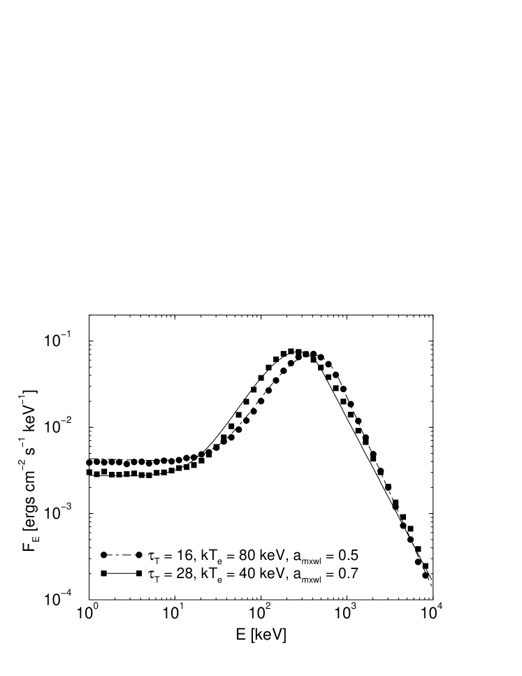
Figure 6: Two typical examples of the analytical representation for Thomson thick Comptonization spectra, using Eqs. (5), (11), (8), (6), and (15) (solid and dot-dashed curves), compared to the Monte-Carlo simulated output spectra (symbols; same simulations as shownin Fig. 1). In both simulations, $p=3.5$ and $\gamma_{2}=10^{3}$ was used.

Table 1: Fit parameters to compute $\langle\gamma-1\rangle$ as a function of the plasma parameters using Eq. 7. $\gamma_{2}=10^{3}$ has been used.

$a_{\rm mxwl}$	$p$	$K_{1}$	$\kappa_{1}$	$K_{2}$	$\kappa_{2}$
0.28	2.20	2.326	0.60	2.329	3.098
0.28	2.48	1.530	0.45	1.332	3.563
0.28	2.73	0.661	0.30	0.876	1.013
0.28	3.00	0.575	0.35	0.662	0.881
0.28	3.24	0.405	0.40	0.576	0.766
0.28	3.50	0.465	0.10	0.249	0.381
0.44	2.20	1.759	0.45	1.761	0.766
0.44	2.48	1.330	0.40	1.007	0.766
0.44	2.73	2.023	0.75	0.761	2.037
0.44	3.00	1.759	0.75	0.576	3.563
0.44	3.24	1.530	0.70	0.435	3.563
0.44	3.50	1.330	0.75	0.379	2.694
0.60	2.20	2.675	0.75	1.332	0.664
0.60	2.48	2.675	0.80	0.761	0.766
0.60	2.73	2.675	0.80	0.501	1.540
0.60	3.00	2.326	0.80	0.379	2.037
0.60	3.24	2.023	0.85	0.329	1.540
0.60	3.50	1.330	0.70	0.249	0.579
0.76	2.20	2.326	0.70	0.761	0.503
0.76	2.48	2.023	0.75	0.435	0.438
0.76	2.73	2.326	0.90	0.329	0.579
0.76	3.00	2.326	0.95	0.249	0.666
0.76	3.24	2.023	0.90	0.188	0.579
0.76	3.50	2.326	0.95	0.164	2.694
0.92	2.20	2.675	0.95	0.249	0.579
0.92	2.48	2.675	1.00	0.164	1.771
0.92	2.73	2.326	1.00	0.108	0.766
0.92	3.00	2.326	1.00	0.081	3.563
0.92	3.24	1.759	0.95	0.062	0.331
0.92	3.50	2.023	1.00	0.054	0.766

References

- Aharonian (1999) Aharonian, F. A., 1999, Astrop. Phys., 11, 225
- Band et al. (1993) Band, D., et al., 1993, ApJ, 413, 281
- Böttcher & Liang (2001) Böttcher, M., & Liang, E. P., 2001, ApJ, 551, in press
- Dermer et al. (1992) Dermer, C. D., Schlickeiser, R., & Mastichiadis, A., 1992, A&A, 256, L27
- Hillas et al. (1998) Hillas, A. M., et al., 1998, ApJ, 503, 744
- Hua & Titarchuk (1995) Hua, X.-M., & Titarchuk, L., ApJ, 449, 188
- Li et al. (1996) Li, H., Kusunose, M., & Liang, E. P., 1996, ApJ, 460, L29
- Liang (1997) Liang, E. P., 1997, ApJ, 491, L15
- Liang (1998) Liang, E. P., 1998, Physics Reports, 302, 67
- Liang et al. (1999) Liang, E. P., et al., 1999, ApJ, 519, L21
- Maraschi et al. (1992) Maraschi, L., Ghisellini, G., & Celotti, A., 1992, ApJ, 397, L5
- Mushotzky et al. (1993) Mushotzky, R. F., Done, C., & Pounds, K. A., 1993, Ann. Rev. A&A, 31, 717
- Pozdnyakov et al. (1983) Pozdnyakov, L. A., Sobol, I. M., & Sunyaev, R. A., 1983, Sovjet Scient. Rev. Section E, Astrophysics and Space Physics Rev., 2, 189
- Rephaeli (1995) Rephaeli, Y., 1995, Ann. Rev. A&A, 33, 541
- Rybicki & Lightman (1979) Rybicki, G. B., & Lightman, A. P., 1979, Radiative Processes in Astrophysics, John Wiley & Sons, New York