Comparison of source detection procedures for XMM-Newton images

Abstract

Procedures based on current methods to detect sources in X-ray images are applied to simulated XMM-Newton images. All significant instrumental effects are taken into account, and two kinds of sources are considered – unresolved sources represented by the telescope PSF and extended ones represented by a $\beta$-profile model. Different sets of test cases with controlled and realistic input configurations are constructed in order to analyze the influence of confusion on the source analysis and also to choose the best methods and strategies to resolve the difficulties.

In the general case of point-like and extended objects the mixed approach of multiresolution (wavelet) filtering and subsequent detection by SExtractor  gives the best results. In ideal cases of isolated sources, flux errors are within 15-20%. The maximum likelihood technique outperforms the others for point-like sources when the PSF model used in the fit is the same as in the images. However, the number of spurious detections is quite large.

The classification using the half-light radius and SExtractor stellarity index is succesful in more than 98% of the cases. This suggests that average luminosity clusters of galaxies ($L_{[2-10]keV}\sim 3\times 10^{44}$ erg/s) can be detected at redshifts greater than 1.5 for moderate exposure times in the energy band below 5 keV, provided that there is no confusion or blending by nearby sources.

We find also that with the best current available packages, confusion and completeness problems start to appear at fluxes around $6\times 10^{-16}$ erg/s/cm² in [0.5-2] keV band for XMM-Newton deep surveys.

1 Introduction

X-ray astronomy has entered a new era now that Chandra and XMM-Newton are in orbit. Their high sensitivities and unprecedented image qualities bear great promises but also pose new challenges. In this paper, we outline problems of object detection in X-ray images that were not previously encountered. In doing so, we compare the performances of various detection techniques on simulated XMM-Newton test images, incorporating the main instrumental characteristics.

The X-ray observations consist of counting incoming photons one by one, recording their time of arrival, position and energy. Later, the event list is used to create images for a given pixel scale and energy band. Various X-ray telescope effects complicate this simple picture – the point spread function (PSF) and the telescope effective area (the vignetting effect), both dependent on the off-axis angle and incoming photon energy; detector effects like quantum efficiency variations, different zones not exposed to X-ray photons; environmental and background effects like solar flares and particle background. Even for relatively large exposures, the X-ray images could contain very few photons, and some sources could contain only a few tens of photons spread over a large area. Consequently, it is important for the source detection and characterization procedures to be able to cope with these difficulties.

As an example, the same hypothetical input situation is shown schematically in Fig. 1 for ROSAT , XMM-Newton  and Chandra  . XMM-Newton ’s rather large PSF, coupled with its higher sensitivity, leads to the detection of more objects but also to blending and source confusion, which become severe for long exposures depending on the energy band. Confusion problems in the hard band above 5 keV are less important, given the smaller number of objects and smaller count rate of energetic photons. Thus, why we concentrate our analysis mainly on source detection problems for the more complicated case of the XMM-Newton energy bands below 5 keV.

Figure 1: Typical representation of objects seen by ROSAT -HRI, XMM-Newton -EPIC and Chandra -HRMA. The objects are represented by $\delta$-functions and folded by the corresponding instrumental PSF and efficiency. Full-width-at-half-maximum (FWHM) of the on-axis PSFs are $1\aas@@fstack{\prime\prime}7$ for ROSAT -HRI, $0\aas@@fstack{\prime\prime}5$ for Chandra -HRMA and $6\arcsec$ for XMM-Newton -EPIC. The dotted line represents schematically the detection limit.

Each X-ray mission provides data analysis packages – EXSAS for ROSAT (Zimmermann et al. exsas (1994)), CIAO for Chandra (Dobrzycki et al. ciao (1999)) and XMM-Newton Science Analysis System (XMM-SAS). They include procedures for source detection, and in this paper we estimate and compare their performances on simulated images using various types of objects. These procedures make use of techniques such as Maximum Likelihood (ML), Wavelet Transformation (WT), Voronoi Tessellation and Percolation (VTP).

In Section 2 we describe the X-ray image simulations. A short presentation of the detection procedures is given in Sec. 3. Tests using only point sources are presented in Sec. 4, and extended sources in Sec. 5. We have analyzed realistic simulations of a shallow and a deep extragalactic field with only point sources in Sec. 6 and with extended objects in Sec. 7 for an exposure of 10 ks. Finally, we investigate the problems of confusion and completeness in two energy bands – [0.5-2] and [2-10] keV for two exposures – 10 ks and 100 ks (Sec. 8). Sec. 9 presents the conclusions. (H${}_{0}=50$ km/s/Mpc, $h=0.5$, q${}_{0}=0.5$ and $\Omega_{0}=1$ are used).

2 Simulation of X-ray images

The simulations are essential to understand and qualify the behavior of the different detection and analysis packages. We have developed a simulation program that generates X-ray images for given exposure times with extended and point-like objects. It takes into account the main instrumental characteristics of XMM-Newton and the total sensitivity of the three EPIC instruments. The procedure is fast and flexible and is made of two independent simulation tasks: object generation (positions, fluxes, properties) and instrumental effects. A possibility to apply the instrumental response directly over images is also implemented, especially useful when one wants to use sky predictions from numerical simulations (cf. Pierre et al. mp00 (2000)).

A summary of the simulated images parameters are given in Tab. 1.

Table 1: The general parameters for the simulated images.

Parameter
Image scale	$4\arcsec$/pixel
Image size	512x512
Exposure time	10ks & 100ks
Energy bands	[0.5-2] & [2-10] keV
PSF on axis	$6\arcsec$ (FWHM)
	$15\arcsec$ (HEW)
Total background (pn+2MOS)
$[0.5-2]$ keV	$1.78\times 10^{-5}$ cts/s/pixel
	0.0041 cts/s/arcmin2
$[2-10]$ keV	$2.4\times 10^{-5}$ cts/s/pixel
	0.0055 cts/s/arcmin2

The point-like sources are assumed to be AGNs or QSOs with a power law spectrum with a photon index of 2 and flux distribution following the $\log N-\log S$ relations of Hasinger et al. (has98 (1998), has01 (2001)) and Giacconi et al. (gia01 (2000)) in the two energy bands.

The PSF model is derived from the current available calibration files. On-board PSF data is generally in very good agreement with the previous ground based calibrations (Aschenbach et al. asch00 (2000)). We must stress that the model PSF is an azimuthal average and in reality, especially for large off-axis angles, its shape can be very distorted. However, in the analytic model (Erd et al. calbook (2000)), the off-axis and energy dependences are not available yet. This is not crucial, as the energy dependence in the bands used is moderate and we confine all the analysis inside $10\arcmin$ from the centre of the field-of-view where the PSF blurring is negligible.

The extended objects are modeled by a $\beta$-profile (Cavaliere & Fusco-Femiano cff76 (1976)) with fixed core radius $r_{c}=250\,h^{-1}$ kpc and $\beta=0.75$. A thermal plasma spectrum (Raymond & Smith rs77 (1977)) is assumed for different temperatures, luminosities and redshifts.

The source spectra (extended and point-like) are folded with the spectral response function for the total sensitivity of the three XMM-Newton EPIC instruments (MOS1, MOS2 and pn with thin filters) by means of XSPEC (Arnaud xspec (1996)) to produce the count rates in different energy bands. The actual choice of the energy bands is not important for this comparison study, although some objects can be more efficiently detected in particular energy ranges.

As an example, we show in Tab. 2 the resulting count rates for extended sources assuming that they represent an average cluster of galaxies.

Table 2: Count rates for extended sources in three energy bands calculated assuming an average luminosity ($L_{[2-10]keV}=2.8\times 10^{44}$ erg/s, $T_{X}=5$ keV) $\beta-$profile cluster of galaxies with a Raymond-Smith spectrum, $N_{H}=5\times 10^{20}$ cm^-2 and spectral response functions for the three EPIC detectors with thin filters.

z	Core radius	Count-rate, photons/s
	arcsec	[0.4-4] keV	[0.5-2] keV	[2-10] keV
0.6	32.8	0.1687	0.1316	0.0362
0.7	31.3	0.1238	0.0963	0.0253
0.8	30.4	0.0942	0.0734	0.0185
0.9	29.7	0.0737	0.0577	0.0139
1.0	29.3	0.0593	0.0465	0.0107
1.1	29.1	0.0486	0.0382	0.0085
1.2	29.0	0.0406	0.0319	0.0068
1.3	29.0	0.0343	0.0270	0.0055
1.4	29.1	0.0293	0.0231	0.0046
1.5	29.2	0.0253	0.0200	0.0038
1.6	29.4	0.0220	0.0175	0.0032
1.7	29.6	0.0193	0.0154	0.0027
1.8	29.9	0.0171	0.0137	0.0023
1.9	30.2	0.0152	0.0122	0.0020
2.0	30.5	0.0137	0.0109	0.0018

The background in the simulations includes realistic cosmic diffuse and background values derived from the XMM-Newton in-orbit measurements in the Lockman Hole (Watson et al. wat00 (2001)).

The calculated count rates for the objects and the photons of the background are subject to the vignetting effect – some photons are lost due to the smaller telescope effective area at given off-axis angle, depending on the incoming photon’s energy. We have parametrized the vignetting factor – the probability that a photon at an off-axis angle $\theta$ to be observed – as polynomials of fourth order in two energy bands: [0.5-2] and [2-10] keV, using the latest XMM-Newton on-flight calibration data. For example, a photon at $\theta=10\arcmin$ has a 53% chance of being observed in [0.5-2] keV and 48% in [2-10] keV.

Further instrumental effects such as quantum efficiency difference between the CCD chips, the gaps between the chips, out-of-time events, variable background, pile-up of the bright sources are not taken into account – their inclusion is not relevant for our main objective.

3 Detection procedures

Without attempting to provide a review of the available techniques in the literature, we briefly describe here the procedures we have tested. They are summarized in Tab. 3.

Table 3: Designation, implementation and short description of the procedures or method used for detection and analysis.

Procedure	Implementation	Version	Method
EMLDETECT	XMM-SAS v5.0	3.7.2	Cell detection + Maximum likelihood
VTPDETECT	Chandra CIAO	2.0.2	Voronoi Tessellation and percolation
WAVDETECT	Chandra CIAO	2.0.2	Wavelet
EWAVELET	XMM-SAS v5.0	2.4	Wavelet
G+SE	Gauss + SExtractor	2.1.6	Mixed – gauss convolution followed by SExtractor  detection
MR/1+SE	MR/1 + SExtractor	2.1.6	Mixed – multi-resolution filtering followed by SExtractor  detection

3.1 Sliding cell detection and maximum likelihood (ML) method

Historically, the sliding cell detection method was first used for Einstein Observatory observations (e.g. EMSS – Gioia et al. emss (1990)). It is included in ROSAT , Chandra and XMM-Newton data analysis tools and a good description can be found in the specific documentation for each of those missions.

The X-ray image is scanned by a sliding square box and if the signal-to-noise of the source centered in the box is greater than the specified threshold value it is marked as an object. The signal is derived from the pixel values inside the cell and noise is estimated from the neighboring pixels. Secondly, the objects and some zone around them are removed from the image forming the so-called “cheese” image which is interpolated later by a suitable function (generally a spline) to create a smooth background image. The original image is scanned again but this time using a threshold from the estimated background inside the running cell to give the map detection object list.

The procedure is fast and robust and does not rely on a priori assumptions. However it has difficulties, especially in detecting extended features, close objects and sources near the detection limit. Many refinements are now implemented improving the sliding cell method: (1) consecutive runs with increasing cell size, (2) matched filter detection cell where the cell size depends on the off-axis angle. However, the most important improvement was the addition of the maximum likelihood (ML) technique to further analyze the detected sources.

The ML technique was first applied to analyze ROSAT observations (Cruddace et al. ml88 (1988), cru91 (1991), Hasinger et al. has93 (1993)). It was used to produce all general X-ray surveys from ROSAT mission (e.g. RASS – Voges et al. rass (1999), WARPS survey – Ebeling et al. warps (2000)). The two lists from local and map detection passes can be merged to form the input objects list for the ML pass. It is useful to feed the ML procedure with as many candidate objects as possible, having in mind that large numbers of objects could be very CPU-expensive. The spatial distribution of an input source is compared to the PSF model – the likelihood that both distributions are the same – is calculated with varying the input source parameters (position, extent, counts) and the corresponding confidence limits can be naturally computed. A multi-PSF fit is also implemented which helps in deblending and reconstructing the parameters of close sources. In the output list, only sources with a likelihood above a threshold are kept.

The ML method performs well and has many valuable features, however, it has some drawbacks – it needs a PSF model to perform the likelihood calculation and thus favours point-like source analysis, extent likelihood could be reliably taken only for bright sources, it cannot detect objects which are not already presented in the input list (e.g. missing detections in the local or map passes).

Here we have used EMLDETECT – an implementation of the method specifically adapted for XMM-SAS (Brunner b96 (1996)). In the map mode sliding cell pass we used a low signal-to-noise ratio ($\sim 3\sigma$) above the background in order to have as many as possible input objects for the ML pass. The likelihood limit (given by $L=-\ln P$, where $P$ is the probability of finding an excess above the background) was taken to be 10, which corresponds roughly to $4\sigma$ detection. A multi-PSF fitting mode with the maximum of 6 simultaneous PSF profile fits was used.

3.2 VTP

VTP – the Voronoi Tessellation and Percolation method (Ebeling & Wiedenmann vtp1 (1993), Ebeling vtp2 (1993)) is a general method for detecting structures in a distribution of points (photons in our case) by choosing regions with enhanced surface density with respect to an underlying distribution (Poissonian in X-ray images). It treats the raw photon distribution directly without any recourse to a PSF model or a geometrical shape of the objects it finds. Each photon defines a centre of a polygon in the Voronoi tessellation image and the surface brightness is simply the inverse area of the polygon (assuming one single photon per cell). The distribution function of the inverse areas of all photons is compared to that expected from a Poisson distribution and all the cells above a given threshold are flagged and percolated, i.e. connected to form an object. This method was successfully used with ROSAT data (Scharf et al. s97 (1997)) and is currently incorporated in the Chandra DETECT package (Dobrzycki et al. ciao (1999)).

Apart from these advantages, VTP has some drawbacks which are especially important for XMM-Newton observations: (1) because of the telescope’s high sensitivity and rather large PSF with strong tails, the percolation procedure tends to link nearby objects; (2) excessive CPU time for images with relatively large number of photons; (3) there is no simple way to estimate the extension of objects.

3.3 Wavelet detection procedures

In the past few years a new approach has been extensively used: the wavelet technique (WT). This method consists in convolving an image with a wavelet function:

$$w_{a}(x,y)=I(x,y)\otimes\psi(\frac{x}{a},\frac{y}{a}),$$ (1)

where $w_{a}$ are the wavelet coefficients corresponding to a scale $a$, $I(x,y)$ is the input image and $\psi$ is the wavelet function. The wavelet function must have zero normalization and satisfy a simple scaling relation

$$\psi_{a}(x,y)=\frac{1}{a}\psi_{1}(\frac{x}{a},\frac{y}{a}).$$ (2)

The choice of $\psi$ is dictated by the nature of the problem but most often the second derivative of the Gaussian function or the so called “Mexican hat” is used.

The WT procedure consists of decomposing the original image into a given number of wavelet coefficient images, $w_{a}$, within the chosen set of scales $a$. In each wavelet image, features with characteristic sizes close to the scale are magnified and the problem is to mark the significant ones, i.e. those which are not due to noise. In most cases, this selection of significant wavelet coefficients cannot be performed analytically because of the redundancy of the WT introducing cross-correlation between pixels. For Gaussian white noise, $w_{a}$ are distributed normally, allowing easy thresholding. This is not the case for X-ray images which are in the Poissonian photon noise regime.

Various techniques were developed for selecting the significant wavelet coefficients in X-ray images. In Vikhlinin et al. (vik97 (1997)) a local Gaussian noise was assumed; Slezak et al. (sle94 (1994)) used the Ascombe transformation to transform an image with Poissonian noise into an image with Gaussian noise; in Slezak et al. (sle93 (1993)), Starck & Pierre (sp98 (1998)) a histogram of the wavelet function is used. In recent years a technique based on Monte Carlo simulations is used successfully (e.g. Grebenev et al. gre95 (1995), Damiani et al. dam97 (1997), Lazzati et al. l99 (1999)).

Once the significant coefficients at each scale are chosen, the local maxima at all scales are collected and cross-identified to define objects. Different characteristics, such as centroids, light distribution etc., can be computed, as well as an indication of the source size at the scale where the object wavelet coefficient is maximal.

WT has many advantages – the multiresolution approach is well suited both for point-like and extended sources but favours circularly symmetric ones. Because of the properties of the wavelet function a smoothly varying background is automatically removed. Extensive description of wavelet transform and its different applications can be found in Starck et al. (sta98 (1998)).

In this work we have tested two WT procedures:

WAVDETECT:

one of the Chandra wavelet-based detection techniques (Freeman et al. fre96 (1996), Dobrzycki et al. ciao (1999)). It uses a “Mexican hat” as wavelet function and identifies the significant coefficients by Monte Carlo simulations. The background level needed to empirically estimate the significance is taken directly from the negative annulus of the wavelet function. Source properties are computed inside the detection cell defined by minimizing the function $|\log r_{PSF}-\log\sigma_{F}|$, where $r_{PSF}$ is the size of the PSF encircling a given fraction of the total PSF flux and $\sigma_{F}$ is the size of the object at the scale closest to the PSF size. No detailed PSF shape information is needed to perform this minimization – just $r_{PSF}$ as a function of the off-axis angle. The control parameters which need attention are the significance threshold and the set of scales. We have used a significance threshold of $10^{-4}$ corresponding to 1 false event in 10000 ($\sim 4\sigma$ in Gaussian case) and “$\sqrt{2}$ sequence” for the scales, where $a=1,\sqrt{2},2,2\sqrt{2},4,3\sqrt{2}\dots 16$.

EWAVELET:

XMM-SAS package, based on a wavelet analysis. It is very similar to WAVDETECT but implements some new ideas. The sources are assumed to have a Gaussian shape in order to analytically derive their counts and extent. Currently, the PSF information is ignored, which can be regarded as a serious drawback. We have used the significance threshold of $10^{-4}$ ($\sim 4\sigma$) and wavelet scales 1, 2, 4, 8 and 16.

3.4 Mixed approach

This method combines a source detection by an elaborated procedure over filtered/smoothed raw photon images.

The use of such a mixed approach is motivated by the fact that procedures for source detection in astronomical images have been developed for many years and the steps and problems of deblending, photometry, classification of objects are now quite well understood. The raw photon image manipulations can be performed with very simple smoothing procedures (for example a Gaussian convolution) or with more sophisticated methods like the “matching filter” technique, adaptive smoothing or multiresolution (wavelet) filtering.

We have used two different types of raw image filtering:

(1)

Gaussian convolution. For our simulated images we applied two convolutions with FWHM=$12\arcsec$ and $20\arcsec$ constrained by the image characteristics (see Sec. 2).

(2)

Multiresolution iterative threshold filtering (MR/1  package, Starck et al. sta98 (1998)) by means of “à trous” (with holes) wavelet method and Poissonian noise model (Slezak et al. sle93 (1993), Starck & Pierre sp98 (1998)) to flag the significant wavelet coefficients (also known as auto-convolution or wavelet function histogram method). The control parameters are the significance threshold, wavelet scales and the number of iterations for the image reconstruction. We took $10^{-4}$ significance threshold (corresponding to $\sim 4\sigma$ for Gaussian distribution), 6 scales for the “à trous” method allowing analysis of structures with characteristic sizes up to $2^{6}$ pixels ($\sim 4\arcmin$). We have used 25 iterations or a reconstruction error less than $10^{-5}$. More iterations can improve the photometry but can also lead to the appearance of very faint real or sometimes false features. Optionally the last-scale wavelet smoothed image in the iterative restoration process is used for analysis of large-scale background variations or very extended features.

Source detection over the filtered images was performed with SExtractor (Bertin & Arnouts sex (1996)) – one of the most widely used procedures for object detection in astronomy with a simple interface and very fast execution time. Originally, SExtractor was developed for optical images but it can be applied very successfully on X-ray images after they are properly filtered. The flexibility of SExtractor is ensured by a large number of control parameters requiring dedicated adjustments. In the following we will briefly outline those having a significant influence on our results:

• Detection and analysis threshold – important parameters for Gaussian convolved images. It is preferable to use a value greater than $4\sigma$, even sacrificing very faint sources but reducing the number of false detections. For MR/1  filtering this is irrelevant because the features in the images are already at $4\sigma$ significance.

• Background mesh size – influences object detection as well as photometry. Using too coarse a background grid (less grid points) will lead to a smoother background image but some faint objects will be missed in the detection. While too detailed a map (more grid points) will lead to many false detections and worse photometry, depending on the local noise properties. We have found after many experiments that local background meshes with 32 to 64 nodes give best results balancing both effects.

• Minimum detection area – in some cases this parameter can help to avoid spurious detections especially when one uses wavelet scales below the characteristic size of objects.

• Deblending parameters – the number of the deblending levels and the minimum contrast. We used the extreme values of 64 levels and zero contrast so that any saddle point will lead to object splitting.

• Photometry – we have decided to use the automatic aperture photometry procedure implemented in SExtractor following Kron (kro80 (1980)) and Infante (inf87 (1987)) which gives better results than the fixed aperture or isophotal methods.

• Classification – we discuss the classification in the next subsection.

3.5 Classification

The problem of classifying sources as resolved or unresolved (or stars/galaxies, extended/point-like) has a long history and discussions can be found in widespread detection packages like FOCAS (Valdes et al. focas (1990)), INVENTORY (Kruszewski inventory (1988)), SExtractor (Bertin & Arnouts sex (1996)), Neural Extractor (Andreon et al. next (2000)). This task becomes even more difficult for X-ray images – we have already mentioned various X-ray telescope effects that blur and distort the images as a function of the off-axis angle.

EMLDETECT

– the extension likelihood is calculated by the deviation of the object fitted from the PSF model when varying the size (extension) of the object. It was used with ROSAT observations to flag possible extended objects and in most of the cases the results were positive. The extension likelihood depends on the chosen PSF model and for faint objects is not reliable (De Grandi et al. sdg97 (1997)).

WAVDETECT

– the ratio between object size and the PSF size ($R_{PSF}$) is used for classification purposes. It depends on the adopted definition for object size and can be misleading, especially for faint objects.

SExtractor

– one parameter for classification is the stellarity index. It is based on neural-network training performed over set of some $10^{6}$ simulated optical images. There are 10 parameters included in the neural network training – 8 isophotal areas, the maximal intensity and the “seeing”. The only controllable parameter is the “seeing” which, however, has no meaning for space observations. It can be tuned to the mean PSF size.
The half-light radius $R_{50}$ is another classification parameter. It can be used as a robust discriminator because it depends only on the photon distribution inside the object (“luminosity profile”), which is assumed to be different for resolved and unresolved objects.

Additional indications might be taken into account when the classification is ambiguous – e.g. the wavelet scale at which object’s wavelet coefficient is maximal or even spectral signatures.

4 Test 1 – point-like sources

4.1 Input configuration

We address the problem of point-like sources separated by $15\arcsec$ (half-energy width of the on-axis PSF), $30\arcsec$ and 60$\arcsec$ with different flux ratios. We include the PSF model and background but do not apply the vignetting effect.

The raw input test image is shown in Fig. 2 together with its Gaussian convolution, MR/1   wavelet filtering and WAVDETECT output image. Visually, the Gaussian image is quite noisy, while there are few spurious detections in the WT images.

Figure 2: Test 1. The raw X-ray photon image with object counts for 10 ks exposure time (upper left). There are three sets of two columns of objects at separations of $15\arcsec$ (HEW of the PSF), $30\arcsec$ and $60\arcsec$. The Gaussian convolution with FWHM$=12\arcsec$ (upper right), MR/1  wavelet filtering (lower left) and WAVDETECT detection image (lower right) both with a significance threshold of $10^{-4}$ are shown.

4.2 Detection rate and positional errors

The number of missing detections and false objects are shown in Tab. 4.

Table 4: Test 1. Detection results. The total number of input objects is 36.

Method	Missed	False
EMLDETECT	4	13
G+SE ($4\sigma$)	6	1
MR/1+SE	7	1
WAVDETECT	7	21
EWAVELET	6	4
VTPDETECT	12	19

The one sigma input-detect position differences are less than the FWHM of the PSF ($6\arcsec$) for all procedures and the maximum occurs for the blended objects, as expected. Note the large number of spurious detections with WAVDETECT, VTPDETECT  and EMLDETECT.

4.3 Photometric accuracy

The results for the photometry in terms of the inferred to the input counts are shown in Fig. 3.

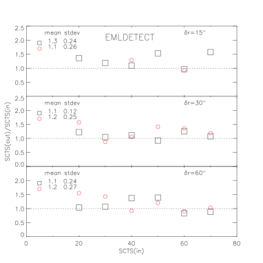
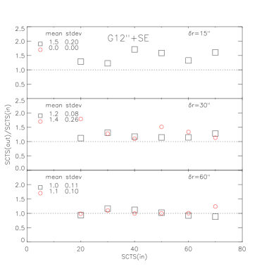
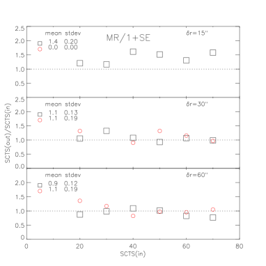
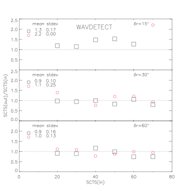
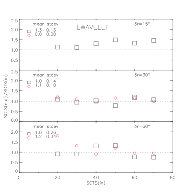
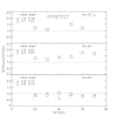
Figure 3: Test 1. The three panels of each figure show the results in terms of the ratio of inferred counts $SCTS(out)$ and input counts $SCTS(in)$ as a function of the varying input counts for the three cases of object separations (indicated by $\delta r$). The mean and st.dev. of the corresponding points are also indicated. When there are no detections, the mean and the st.dev. are both zero. Objects with input counts fixed at 100 (squares) are placed beside their corresponding neighbors (circles), rather than being plotted at 100.

$\delta r=15\arcsec$.

Only EMLDETECT detects two of the six fainter objects. None of the other procedures separates the objects and consequently the inferred counts are a blend from both sources.

$\delta r=30\arcsec$.

The proximity of objects influences the detection and the photometry. EMLDETECT and EWAVELET show the best detection rate results while all the other procedures miss one of the faintest objects.

$\delta r=60\arcsec$.

We can safely assume that the objects are well separated. The recovery of the properties is informative for the performance of the tested procedures. It is clear that the general flux reconstruction error (taken to be the spread of the points around the unity line in Fig. 3) is about 15% for brighter sources and goes down to 20-25% for the faintest ones. [In our 10 ks exposure tests and with the adopted background in band [0.5-2] keV, we assume the objects with input counts of 20 photons ($\sim 10^{-15}$ erg/s/cm²) to be at the detection limit when there is no confusion by nearby sources.]

4.4 Discussion

After this simple test we can eliminate the VTPDETECT: in addition to the very large execution time, some of the VTP-detected object centres were shifted by more than $20\arcsec$ from their input positions – a consequence of its ability to detect sources with different shapes where the object center can be far from the input position. Moreover, VTPDETECT percolates all the double sources into single objects at $\delta r=30\arcsec$, which all other procedures were able to separate.

No procedure unambiguously shows best results – both in terms of the detection rate, spurious sources and photometric reconstruction. EMLDETECT outperforms the others in terms of detection rate but with the price of many spurious detections. Using exactly the same PSF model as the one hard-coded in EMLDETECT leads to much better photometric reconstruction.

All other procedures are comparable: EWAVELET showing better detection but its photometric reconstruction is far from satisfactory – about half of the photons were lost at $\delta r=30\arcsec$ and $60\arcsec$, because of the assumed Gaussian shape used to derive analytically extension and counts. We have applied a simple correction for the object size to arrive at the good photometric results for EWAVELET presented on Fig. 3.

5 Test 2 – point-like plus extended objects

5.1 Input configuration

This test is similar to Test 1, but we have replaced some of the point-like sources by extended ones generated as described in Sec. 2. The raw photon image with input counts indicated and its representations are shown in Fig. 4.

Figure 4: Test 2. The raw X-ray photon image for 10 ks exposure time (upper left). As in Fig. 2 three cases of separations are indicated, as well as the corresponding input source counts. The extended objects are in the right columns. The Gaussian convolution with FWHM$=20\arcsec$ (upper right), MR/1  WT filtered image (lower left) and WAVDETECT reconstructed image both with a significance threshold of $10^{-4}$ (lower right) are shown.

5.2 Detection rate and positional errors

The number of missed and false detections are shown in Tab. 5. An increase of the searching radius to $20\arcsec$ was needed: at $\delta r=15\arcsec$ the blending tends to shift the centroid towards the point-like source. Note that this situation is a clear case for source confusion: if we take the closest neighbour (the point-like source in some cases) as the cross-identification from the input list, we shall overestimate the flux more than two-fold, while the true representation is the extended object.

Some changes were needed for the procedures not based on the wavelet technique in order to avoid splitting of the bright extended objects into sub-objects: increase of the Gaussian convolution FWHM to $20\arcsec$, and multi-PSF fit for EMLDETECT. In the Gaussian case, the larger smoothing length smears some of the point-like sources, leading to non-detection. EMLDETECT splitting persists even with the maximum number of the PSFs fitted to the photon distribution (currently it is capable of simultaneously fitting up to 6 PSFs).

Table 5: Test 2 results for the detection rate. The first number in the “Missed” column is for point sources while the second is for extended ones. The total number of input sources is 24=12+12.

Method	Missed	False
EMLDETECT	1+1	89
G+SE $4\sigma$	6+0	1
MR/1+SE	6+0	6
WAVDETECT	6+0	18
EWAVELET	4+2	5

5.3 Photometric reconstruction

The inferred-to-input source counts ratio $SCTS(out)/SCTS(in)$ is shown in Fig. 5. We will not consider EWAVELET  as its photometric results and detection of extended sources were quite unsatisfactory. The simple correction technique (as in Test 1) based on the PSF does not work – the extended objects profile has different shape from the PSF.

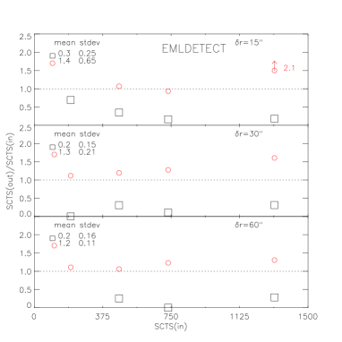
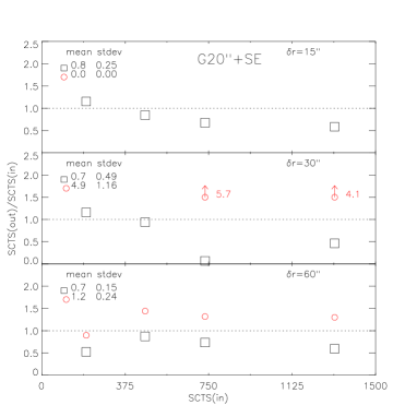
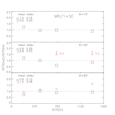
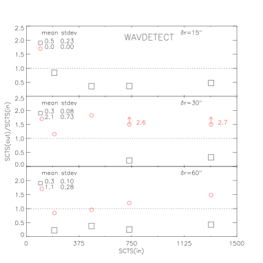
Figure 5: Test 2. As in Fig. 3 except that the squares now represent extended objects and the point-like sources at fixed counts of 100 (circles) are put beside their corresponding neighbors (rather than being put at 100). Circles with arrows and numbers denote the ratio when it is above 2.

$\delta r=15\arcsec$.

Only MR/1+SE gives good results for the flux restoration of the extended objects, but overestimating the counts for the faintest one. WAVDETECT misses almost half of the input photons while EMLDETECT splitting leads to very poor results.

$\delta r=30\arcsec$.

All procedures give bad restoration results with MR/1+SE performing best again for the extended sources. The proximity of the objects leads to an overestimation of the point-like source counts and an underestimation of the extended object counts. There is no simple way to correct for this effect, but can be done using a rather elaborated iterative procedure involving extended object profile fitting.

$\delta r=60\arcsec$.

Point-like source results are relatively similar with all procedures – the source counts are slightly overestimated due to the extended object halo even at $60\arcsec$. The problems of WAVDETECT and EMLDETECT and the recovery of the extended objects counts are quite obvious. Again MR/1+SE is the best performing procedure with extended objects flux uncertainty about 25-30%.

5.4 Object classification

An important test is the ability of the procedures to classify objects and to allow further analysis of complicated cases of blending. The MR/1+SEresults for the clasification by means of the half-light radius and stellarity index (c.f. Sec. 3.5) are shown in Fig. 6, overlayed over the results from 10 simulated images with only point-like sources. Clearly the detected extended objects with MR/1+SE fall into zones not occupied by point-like sources. Note, however, that the two detected point-like sources at $30\arcsec$ will be mis-clasified as extended objects – the proximity not only influences the source counts, overestimated by more than 4-5 times (Fig. 5), but also the object profile and consequently the classification.

Fig. 7 shows the WAVDETECTclassification – the ratio of the object size to the PSF size ($R_{PSF}$). The results are more ambiguous with WAVDETECT (Fig. 7) compared to MR/1+SE. The results with EMLDETECT and its classification parameter (extension likelihood) were very unsatisfactory due to the extended object splitting. More comprehensive discussion of the simulations and the classification is left for Sec. 7.

Figure 6: Test 2. MR/1+SE  detection classification based on $R_{50}$ (left panels) and stellarity (right panels) as a function of the off-axis angle (upper panels) and detected source counts (lower panels). Identified extended (filled circles) and point-like objects (triangles) are plotted over the results from 10 simulated images with only point-like sources (see Sec. 6).

Figure 7: Test 2. WAVDETECT  classification based on object size to PSF size ratio – $R_{PSF}$. The identified extended (filled circles) and point-like sources (triangles) are plotted over the results from 10 simulated images with only point-like sources (see Sec. 6), the dashed line marks a ratio of unity .

5.5 Discussion

Clearly EMLDETECT and WAVDETECT have problems in restoring the fluxes of extended objects. We have already discussed the splitting difficulties of EMLDETECT. The explanation for WAVDETECT’s bad results is that the wavelet scale at which the detected object size is closer to the PSF size defines the source detection cell (in which the flux is computed). If the characteristic size of an object is larger than the PSF size (i.e. an extended object) this procedure will tend to underestimate the flux.

We can safely accept the MR/1+SE procedure as the best performing for detection and characterization both for point-like and extended objects. We must stress however that one cannot rely on the flux measurements when there are extended and point-like sources separated by less than $30\arcsec$. The proximity affects also the classification of the point-like sources. Using the classification and then performing more complicated analysis like profile fitting and integration for the extended sources can improve a lot the restoration. In realistic situations we can expect very often problems of this kind, especially with XMM-Newton .

6 Test 3 – Realistic model with only point-like sources

6.1 Input configuration

We simulate an extragalactic field including only point-like sources with fluxes drawn from the $\log N-\log S$ relation (Hasinger et al. has98 (1998), has01 (2001), Giacconi et al. gia01 (2000)). PSF, vignetting and background models are applied as described in Sec. 2. The aim is to test the detection procedures in more realistic cases where confusion and blending effects are important and not controlled. The raw photon image is shown in Fig. 8 together with its visual representation – the same input configuration for a much larger exposure time and no background, only keeping the objects with counts greater than 10. It displays better the input object sizes, fluxes and positions and it is instructive to compare it to the MR/1  filtered and WAVDETECT images shown on the same figure.

Figure 8: Test 3. A simulated XMM-Newton extragalactic field with only point-like sources for 10ks exposure time and the total sensitivity of the three EPIC instruments (upper left), its representation for much larger exposure time and no background (upper right). The MR/1+SE filtering (lower left) and WAVDETECT  images both with $10^{-4}$ significance threshold (lower right) are shown.

6.2 Cross-identification and positional error

We need to define a searching radius in order to cross-identify the output and the input lists. The input list contains many objects with counts well below the detection limit ($\log N-\log S$ extends to very faint fluxes) and a lower limit must be chosen. For each detected object, we search for the nearest neighbour inside a circle within the reduced input list.

The positional difference for the brightest detected sources (more than 100 counts) in the inner $10\arcmin$ from the center of the FOV is shown in Tab. 6. The region beyond $10\arcmin$ is subject to serious problems caused by the vignetting and PSF blurring, the detected object centroid can be few PSFs widths from the true input identification.

We therefore adopt the following cross-identification parameters: the input list is constrained to counts greater than 10; a $6\arcsec$ searching radius; we consider only the central $10\arcmin$ of the FOV.

Table 6: One sigma positional error and number of detected objects inside the inner $10\arcmin$ from the center of the FOV and more than 100 counts for a 10 ks exposure.

Procedure	$\Delta r\arcsec$	number
EMLDETECT	2.9	13
G+SE	3.5	14
MR/1+SE	3.2	13
WAVDETECT	4.1	12

6.3 Detection rate and photometric reconstruction

The detection rate and flux reconstruction results are shown in Fig. 9. There are different effects playing a role in the distribution and the numbers of missed and false detections:

(1)

“false” detections – non-existent objects, or two or more sources blended into a single detected object. The result will be a “false” detection if the blended objecs are not in the input list (count limit) or the merged object centroid is beyond the searching radius.

(2)

source confusion – in the cross-identification process the nearest neighbour to the detected source is not the true assignment; or as in case (1), when a blend of objects is wrongly identified by one input source.

(3)

missed detections – depending on the local noise properties, some objects can be missed even if their input counts are above the adopted limiting counts for cross-identification.

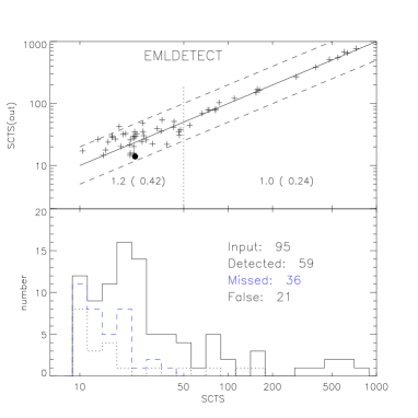
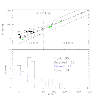
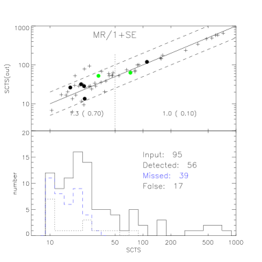
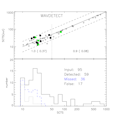
Figure 9: Test 3. Recovery of the input flux (upper panel of each figure). The continuous line is exact match between detected and input counts while the dashed lines are for two times differences. The limit of 50 input counts is shown by a vertical dotted line and the mean and the st.dev. (in brackets) of $SCTS(out)/SCTS(in)$ for the two regions are indicated. The black circles denote objects with detect-input position difference larger than $4\arcsec$, suggesting blending effects; the grey circles denote objects with more than one neighbour inside the searching radius. In the bottom panels, the corresponding rate and distribution of input counts (continuous histogram), missed input objects (dashed histogram) and possible false detections (dotted histogram) are shown.

6.4 Discussion

The results in terms of detection rate are similar for all procedures. The best detection rate shows G+SE  but at the price of twice as many false detections.

The photometry reconstruction for the sources above 50 counts shows a spread about 10-15% for the WT based methods and $\sim 25\%$ for EMLDETECT. However, EMLDETECT clearly outperforms the other procedures when we use the same PSF model as the one hard-coded into the programme. This fact shows that using a correct PSF representation has a crucial importance for the ML technique. More discussion about the detection limits, completeness and confusion is left for Sec. 8.

7 Test 4 – sky models with point-like and extended objects

7.1 Input configuration

We have chosen exactly the same input point-like sources configuration as in Test 3 and we have added 5 extended objects. They may be regarded as clusters of galaxies at different redshifts with the same $\beta$-profiles and moderate X-ray luminosity $L_{[2-10]keV}\sim 3\times 10^{44}$ erg/s (c.f. Tab. 2). Now the objective is to estimate the capabilities of the procedures to detect and identify extended objects. The difference from Test 2 is the arbitrary positions of the point-like sources leading to different local and global background properties and to uncontrolled confusion effects.

The input configuration and wavelet filtered and output images are given in Fig. 10.

Figure 10: Test 4. The raw X-ray photon image with point-like and extended objects for 10ks exposure time (upper left) and its visual representation for much larger exposure and no background (upper right). The corresponding redshifts for the clusters are indicated. The MR/1+SE  filtering (lower left) and WAVDETECT  both with $10^{-4}$ significance threshold (lower right) are shown.

7.2 Positional and photometric reconstruction

Results for the point-like sources will not be presented, because the input configuration (position, $\log N-\log S$, background) is exactly the same as in the previous test. It was shown in Test 2 that the presence of a point source even with moderate counts in the vicinity of a faint extended source could lead to confusion and even non-detection. Of course, the presence of a cluster will affect the detection and photometry of the point-like objects in its vicinity, but this effect is of minor concern for this test and has been already discussed (Test 2).

The detection rate, input-detect position offsets, detected counts and detected-to-input counts ratio are shown in Tab. 7.

Table 7: Recovery of position and flux of the extended objects.

redshift	$\Delta r$	Input	Detect	Detect/Input
	[arcsec]	[counts]	[counts]	[%]
EMLDETECT
0.6	2.1	1316	94	7
1.0	8.0	465	12	3
1.5	12.3	200	161	81
1.8	4.6	136	228	167
2.0	14.8	109	32	29
G+SE
0.6	1.2	1316	1043	79
1.0	5.2	465	355	76
1.5	1.9	200	220	110
1.8	Not detected
2.0	15.3	109	80	73
MR/1+SE
0.6	0.2	1316	1016	77
1.0	2.3	465	340	73
1.5	1.8	200	223	111
1.8	11.8	136	83	61
2.0	10.8	109	185	169
WAVDETECT
0.6	5.8	1316	344	26
1.0	10.6	465	193	41
1.5	0.1	200	39	19
1.8	Not detected
2.0	15.3	109	27	24

As to the positional errors, it was already concluded that the centres of the extended object can be displaced by more than the adopted searching radius for point-like sources (Sec. 5). The differences in positions shown in Tab. 7, especially for fainter objects, are 3-4 times larger than the one sigma limit for point-sources inside the inner $10\arcmin$ of the FOV (Tab. 6).

It is confirmed again that EMLDETECT and WAVDETECT are not quite successful in charactering extended objects. But note that this time the results for MR/1+SE and G+SE  are worse than the results in Test 2 – the rate of lost photons being about 20-30%. Also, the flux of the clusters at $z=1.5$ and $2$ is overestimated, suggesting blending with faint nearby point-like sources.

7.3 Classification

To classify the detected objects we have performed many simulations with only point-like sources as in Test 3. Ten simulated images were generated with the same $\log N-\log S$ and background, but with different and arbitrary positions of the input sources. Exactly the same parameters were used for filtering, detection and characterization.

Two classification parameters were used: the half-light radius ($R_{50}$) and the stellarity index from SExtractor based procedures. The results are shown in Fig. 11. We do not show results with WAVDETECT and EMLDETECT classification parameters because their unsatisfactory results were confirmed, as in Test 2.

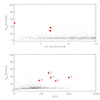
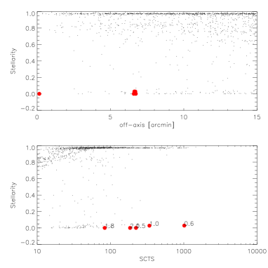
Figure 11: Test 4. Half-light radius $R_{50}$ (left figures) and stellarity index (right) as a function of the off-axis angle (up) and detected counts (down) for 10 generations. The detection was performed with SExtractor  after MR/1   multiresolution filtering. There are in total 1287 detections indicated by points. The extended objects from this test are shown with filled circles.

We can see the excellent classification based on the stellarity index and half-light radius: in the inner $10\arcmin$, for objects with more than 20 detected counts, stellarity less than 0.1 and $R_{50}\geq 20\arcsec$ we have 15 incorrect assignments from 1287 detections ($\sim 1\%$).

8 Test 5 – completeness and confusion

In this section we investigate the confusion and completeness problems for XMM-Newton shallow and deep observations like the first XMM Deep X-ray Survey in the Lockman Hole (Hasinger et al. has01 (2001)).

A set of 10 images with exposure times of 10 ks and 100 ks in the energy bands [0.5-2] and [2-10] keV were generated; the fluxes were drawn using the latest $\log N-\log S$ relations from Hasinger et al. (has01 (2001)) and Giacconi et al. (gia01 (2000)). Detection and analysis were performed with exactly the same parameters for all simulations: detection threshold, analysis threshold, background map size, detection likelihood, etc. (see Sec. 3). Cross-identification was achieved using the input sources above 10 counts and 30 counts for 10 ks and 100 ks exposures respectively. Lowering the count limits yields more cross-identifications but increases considerably the number of spurious detections.

The input image for 100 ks and [0.5-2] keV band is shown in Fig. 12. The inner $10\arcmin$ zone where all analysis is performed is indicated, as well as the total XMM-Newton field-of-view. It is informative to compare it with the images for 10 ks in Fig. 8.

Figure 12: Simulated 100ks XMM-Newton deep field in [0.5-2] keV with the same parameters ($N_{H},\ \log N-\log S,\ \Gamma$, background) as in the Lockman Hole (Hasinger et al. has01 (2001), Watson et al. wat00 (2001)). We restrict the analysis to the inner $10\arcmin$.

In order to estimate the effect of confusion we have generated images with only point-like sources, distributed on a grid such to avoid close neighbours, and with fixed fluxes spanning the interval $[10^{-16},10^{-13}]$ erg/s/cm².

In the following we discuss some important points.

• Confusion and completeness
  The detection rate of the input sources as a function of flux (Fig. 13) indicates that confusion problems are significant for 100 ks exposures in the [0.5-2] keV band. They are marginal for 100 ks exposures in [2-10] keV band and absent for 10 ks in both bands.

  

  

  Figure 13: Ratio of number of cross-identified objects to the number of input objects, with counts greater than 10 and 30 for 10 ks and 100 ks exposures respectively, as a function of the input flux. The results of 10 generations are shown by crosses, the heavy histogram is the corresponding average; the curve indicates the detection rate if confusion is absent and the dotted line marks 90% completeness.

  Energy conversion factors and the limiting fluxes below which more than 10% of the input objects are lost are shown in Tab. 8.

  Table 8: The energy conversion factors (ECF) and the 90% completeness limits for detections. ECF is computed assuming power-low spectrum with photon index $\Gamma=2,\ N_{H}=5\times 10^{19}$ cm^-2 (Hasinger et al. has01 (2001)) and the three EPIC instruments (pn+2MOS) with thin filters.

  	[0.5-2] keV	[2-10] keV
  ECF (cts/s per erg/s/cm2)
  	$6.70\times 10^{-13}$	$3.66\times 10^{-12}$
  Flux limits (erg/s/cm2)
  10ks	$2\times 10^{-15}$	$10^{-14}$
  100ks	$6\times 10^{-16}$	$3\times 10^{-15}$

• Differential flux distribution
  The differential flux distributions for 100 ks in [0.5-2] keV obtained by MR/1+SE and EMLDETECT are shown on Fig. 14. Spurious detections appears to be numerous with EMLDETECT below $5\times 10^{-16}$ erg/s/cm² and tend to compensate the loss of sensitivity and confusion. MR/1+SE appears to be less affected and allows us to set a conservative flux limit of $6\times 10^{-16}$ erg/s/cm²($\sim 90$ photons for 100 ks), below which the incompleteness becomes important – 65% of the input sources are lost between $3\times 10^{-16}$ and $6\times 10^{-16}$ erg/s/cm².

  

  Figure 14: Differential number counts as a function of flux. The continuous histogram is the input distribution, the dots with error bars (Poissonian) are the measured distribution (without any cross-identifications) and the dashed histogram indicates the false detections – all are averaged from 10 simulations. Left for MR/1+SE, right for EMLDETECT.

• $\log N-\log S$
  The $\log N-\log S$ functions in [0.5-2] keV for 10 ks and 100 ks exposures are shown in Fig. 15. The inferred $\log N-\log S$ (by simple source counting) are in very good agreement with the input ones down to fluxes about $2\times 10^{-15}$ and $6\times 10^{-16}$ erg/s/cm² with MR/1+SEand $10^{-15}$ and $3\times 10^{-16}$ erg/s/cm² for EMLDETECTfor 10 ks and 100 ks respectively. Although there are confusion and completeness problems for 100 ks starting at $5-6\times 10^{-16}$ erg/s/cm²as discussed above, their effect is completely masked in the EMLDETECT integral distribution, which seems to be in very good agreement down to $3\times 10^{-16}$ erg/s/cm²(the lower flux limit for the Lockman Hole Deep Survey analysis of Hasinger et al. has01 (2001)).

  

  Figure 15: The integral number of objects in the inner $10\arcmin$ (surface 0.087 sq.deg.) as a function of the flux for [0.5-2] keV and two exposures: 10 ks and 100 ks. The points with error bars (Poissonian) are the detections (without cross-identification) with MR/1+SE  boxes are EMLDETECTresults, while the histogram is the input $\log N-\log S$ function.

• Photometric accuracy
  The photometric reconstruction is relatively similar for 10ks and 100ks in for fluxes greater than $2\times 10^{-15}$ and $6\times 10^{-16}$ erg/s/cm² respectively (the 90% completeness limit, Fig. 16). The flux uncertainties are about 25-30 % and going down to fainter fluxes leads to very poor photometry.

  

  Figure 16: Photometry reconstruction for all 10 simulated images at 10 ks (left) and 100 ks (right) in the [0.5-2] keV band. The solid line is exact match between detected and input counts while the dashed lines are for two-fold differences. The vertical dashed line marks the 90% completeness limit (see Tab. 8) and mean and st.dev. (in brackets) above this limit are denoted.

9 Conclusions

Various procedures for detecting and characterizing sources were tested by simulated X-ray images. We have concentrated our attention mainly on images with XMM-Newton specific characteristics, because the problems arising from its high sensitivity and relatively large PSF are new and challenging.

We have analyzed the detection rate and the recovery of all characteristics of the input objects: flux, positional accuracy, extent measurements and the recovery of the input $\log N-\log S$ relation. We have also investigated confusion problems in large exposures.

Concerning detection rate and characteristics reconstruction, we have shown that the VTPDETECT implementation of the Voronoi Tessellation and Percolation method is not suited to XMM-Newton images. EWAVELET provides very good detection rate and photometric reconstruction for point-like sources after a simple correction, but shows unreliable results for extended sources.

One of the best methods for point-like source detection and flux measurements is EMLDETECT but we stress again that the PSF model used for the ML procedure needs to be close to the image PSF for the most accurate photometry. Serious drawbacks are the relatively large number of spurious detections as well as the splitting of the extended sources, which we were not able to suppress even with 6 simultaneous PSF profile fits in the multi-PSF mode; this seriously hampers the analysis of the extended sources.

WAVDETECT is a flexible method giving good detections even in some complicated cases. But, here again, spurious detections are quite numerous. WAVDETECT does not assume a PSF model but requires the PSF size as a function of the encircled energy fraction and the off-axis distance in order to define the object detection cell. However, the way the detection cell is defined leads to bad photometry for extended objects.

Our choice is the MR/1+SE method. The mixed approach involving first a multiresolution iterative threshold filtering of the raw image followed by detection and analysis with SExtractor. Our tests have shown that this is the best strategy for detecting and characterizing both point-like and extended objects . Even though this mixed approach consists of two distinct steps, it is one of the fastest procedures (Tab. 9), allowing easy checks of different stages in the analysis (filtering, detection, photometry).

Table 9: CPU times for performing Test 5 for 100ks. The procedures were run on a Pentium III-Xeon, 550MHz, Linux. G+SE   and MR/1+SE  CPU time is the total of filtering and detection passes. For EMLDETECT  the number of input objects is given.

Procedure	Number of	CPU time
	detections	[min.]
EMLDETECT	528	12.0
EWAVELET	364	0.4
MR/1+SE	370	1.9
G+SE	365	0.1
WAVDETECT	378	10.3
VTPDETECT	1307	10.7

Without blending or confusion effects, the photometry is accurate within 10-20% for both point-like and extended objects. This uncertainty can be regarded as an intrinsic error due to the Poissonian nature of the X-ray images. For extended objects, only the MR/1+SE method gives satisfactory photometric results.

Blending between extended and point-like sources is quite serious at separations below $\sim 30\arcsec$. Better results for photometry may eventually be obtained if the intrinsic shape of the extended objects is known, and if the two objects are detected. However, in most of the cases with small separation, there is no indication of blending – which is a dangerous situation for flux reconstruction. In such cases, there may exist some spectral signatures of the effect.

The identification process of X-ray sources relies on their positional accuracy. We have shown that for objects with more than 100 counts in 10 ks exposure images and within the inner $10\arcmin$ of the field-of-view, the one sigma positional error is of the order of one half of the FWHM of the PSF ($\approx 3-4\arcsec$, Tab. 6). For extended objects, because of their shallower profiles and depending on the number of photons and the off-axis distance, the detected centre could even be at about $15\arcsec$ from its input position.

Comparing series of simulations with 100 ks and 10 ks in two energy bands – $[0.5-2]$ and $[2-10]$ keV, we show that the effects of confusion and completeness are absent for 10 ks, but quite significant for 100 ks in the lower energy band. Moreover, for faint fluxes, these effects tend to be masked by the large number of spurious detections with EMLDETECT. Although this method seems to give correct results for the $\log N-\log S$ down to fainter fluxes than MR/1+SE, in real situations it is impossible to asses the contribution of the numerous spurious detections. From our simulations, we estimate that about 60-65% of the sources are lost between $3\times 10^{-16}$ and $6\times 10^{-16}$ erg/s/cm² for a 100 ks exposure with the current best method (MR/1+SE).

One of the most important conclusions that will have deep cosmological impact concerns the detection and classification of extended objects. We have shown that the MR/1+SE mixed approach is capable of detecting galaxy cluster-like objects with moderate luminosity ($L_{[2-10]keV}\sim 3\times 10^{44}$ erg/s) at redshifts $1.5<z<2$ in 10 ks XMM-Newton simulated images. A criteria based on the half-light radius and the stellarity index classifies them correctly, with a confidence level greater than 98%.

- (1) Andreon S., Gardiulo G., Longo G., et al, 2000, MNRAS, 319, 700 (NExt)
- (2) Arnaud K.A., 1996, in ASP Conf. Ser., Vol. 101, Astronomical Data Analysis Software and Systems V,eds. Jacoby G.H. & Barnes J. (San Francisco: ASP), 17 (XSPEC)
- (3) Aschenbach B., Briel U., Haberl F., et al., 2000, SPIE 4012, 731 (astro-ph/0007256)
- (4) Bertin E., Arnouts S., 1996, A&AS 117, 393 (SExtractor)
- (5) Brunner H., 1996, Technical Note (SSC-AIP-TN-0001), http://xmmssc-www.star.le.ac.uk/documents/
- (6) Cavaliere A., Fusco-Femiano R., 1976, A&A 49, 137
- (7) Cruddace R.G., Hasinger G.R., Schmitt J.H., 1988, In: Astronomy from large databases, eds. F. Murtagh & A. Heck (Garching:ESO)
- (8) Cruddace R.G., Hasinger G.R., Trümper J. et al., 1991, Exp.Astron. 1, 365
- (9) Damiani F., Maggio A., Micela G., Sciortino S., 1997, ApJ 483, 350
- (10) De Grandi S., Molendi S., Bḧoringer H., et al., 1997, ApJ 486, 738
- (11) Dobrzycki A., Ebeling H., Glotfelty K. et al., 1999, In Chandra DETECT User Guide: http://asc.harvard.edu/
- (12) Erd C., Gondoin P., Lumb D., et al., 2000, XMM Calibration Access and Data Handbook, XMM-PS-GM-20 Issue 1.1, http://xmm.vilspa.esa.es/calibration/
- (13) Giacconi R., Rosati P., Tozzi P. et al., 2000, astro-ph/0007240v2
- (14) Gioia I.M., Maccacaro T., Schild R.E., et al., 1990, ApJSS 72, 567
- (15) Grebenev S.A., Forman W., Jones C., Murray S., 1995, ApJ 445, 607
- (16) Ebeling H., 1993, Ph.D. thesis, MPE Report 250.
- (17) Ebeling H., Wiedenmann G., 1993, Phys. Rev. 47, 704
- (18) Ebeling H., Jones L.R., Perlman E., et al., 2000, ApJ 534, 133
- (19) Freeman P., Kashyap V., Rosner R. et al., 1996, in ASP Conf. Ser., Vol. 101, Astronomical Data Analysis Software and Systems V, eds. Jacoby G.H. & Barnes J. (San Francisco: ASP), 163
- (20) Hasinger G., Burg R., Giacconi R., et al., 1993, A&A, 275, 1 (erratum 1994, A&A 291, 348)
- (21) Hasinger G., Burg R., Giacconi R., et al., 1998, A&A, 329, 482
- (22) Hasinger G., Altieri B., Arnaud M., et al. 2001, A&A, 365, L45
- (23) Infante L., 1987, A&A 183, 177
- (24) Kolaczyk E., Dixon D., 2000, ApJ 534, 490
- (25) Kron R.G., 1980, ApJS 43, 305
- (26) Kruszewski, A., 1988, in 1st. ESO/ST-ECF Data Analysis Workshop, eds. Grosbol P.J., Murtagh F., Warmels R.H., ESO Munchen, 29
- (27) Lazzati D., Campana S., Rosati P., et al., 1999, ApJ 524, 414
- (28) Pierre M., Bryan G., Gastaud R., 2000, A&A 356, 403
- (29) Raymond J.C., Smith B.W., 1977, ApJS 35, 419
- (30) Scharf C.A., Jones L.R., Ebeling H., et al., 1997, ApJ 477, 79
- (31) Slezak E., de Laparent V., Bijaoui A., 1993, ApJ 409, 517
- (32) Slezak E., Durret F., Gerbal D., 1994, AJ 108, 1996
- (33) Starck J.-L., Pierre M., 1998, A&AS 128, 397
- (34) Starck J.-L., Murtagh F., Bijaoui A., 1998, Image Processing and Data Analysis: The Multiscale Approach, Cambridge Univ. Press, Cambridge (UK) (MR/1 )
- (35) Valdes F.G., Campusano L.E., Velasquez J.D., Stetson P.B., PASP 107, 1119 (FOCAS)
- (36) Vikhlinin A., Forman W., Jones C., 1997, ApJ 474, L7
- (37) Voges W., Aschenbach B., Boller Th., et al., 1999, A&A 349, 389
- (38) Watson M.G., Auguères J.-L., Ballet J., et al. 2001, A&A, 365, L51
- (39) Zimmermann H.U., Becker W., Belloni T., et al., 1994, EXSAS User’s Guide, MPE Report 257 (EXSAS)