Chandra Observation of RXJ1720.1+2638: a Nearly Relaxed Cluster with a Fast Moving Core?

Abstract

We have analyzed the Chandra observation of the distant ($z=0.164$) galaxy cluster RXJ1720.1+2638  in which we find sharp features in the X-ray surface brightness on opposite sides of the X-ray peak: an edge at about $250~{}h_{50}^{-1}$ kpc to the South-East and a plateau at about $130~{}h_{50}^{-1}$ kpc to the North-West. The surface brightness edge and the plateau can be modeled as a gas density discontinuity (jump) and a slope change (break). The temperature profiles suggest that the jump and the break are the boundaries of a central, group-size ($d\approx 380h_{50}^{-1}$ kpc), dense, cold ($T\approx 4$ keV) gas cloud, embedded in a diffuse hot ($T\approx 10$ keV) intracluster medium. The density jump and the temperature change across the discontinuity are similar to the “cold fronts” discovered by Chandra  in A2142 and A3667, and suggest subsonic motion of this central gas cloud with respect to the cluster itself. The most natural explanation is that we are observing a merger in the very last stage before the cluster becomes fully relaxed. However, the data are also consistent with an alternative scenario in which RXJ1720.1+2638  is the result of the collapse of two co-located density perturbations, the first a group-scale perturbation collapse followed by a second cluster-scale perturbation collapse that surrounded, but did not destroy, the first one. We also show that, because of the core motion, the total mass inside the cluster core, derived under the assumption of hydrostatic equilibrium, may underestimate the true cluster mass. If widespread, such motion may partially explain the discrepancy between X-ray and the strong lensing mass determinations found in some clusters.

1 INTRODUCTION

In the hierarchical cosmological scenario, clusters of galaxies grow through gravitational infall and merging of smaller groups and clusters (e.g. White & Rees 1978; Davis et al. 1985). The process may be described as a sequence of merging and relaxation phases in which substructures are alternatively accreted and merged into the larger system. To date it is not clear to what extent subclumps of matter, that have already collapsed prior to infall into a larger cluster, can survive. Analytic calculations, for example, suggest that groups of galaxies may not survive in a larger cluster environment for more than one crossing time after which they will be tidally disrupted (see e.g. González-Casado, Mamon, & Salvador-Sole 1994). However, recent high resolution N-body simulations show that galaxy-like and group-like halos form and may survive even in central cluster cores (Moore et al. 1999; Ghigna et al. 1999; Klypin et al. 1999).

We present a Chandra  observation of the cluster of galaxies RXJ1720.1+2638  that may exhibit just such a surviving halo in its center. This cluster was first observed in X-rays by the Einstein IPC in a project devoted to the study of the X-ray emission from radio sources with steep spectra (Harris et al. 1988). It was subsequently observed with ASCA  but, to date, there are no published papers on the analysis of these data, and thus, we performed our own ASCA  spectral analysis. Among the galaxy members only the redshift of the central galaxy is known ($z=0.164\pm 0.004$) (Harris et al. 1988; Crawford et al. 1999).

The Chandra  data show a sharp edge in the X-ray surface brightness produced by a density discontinuity at about $250~{}h_{50}^{-1}$ kpc SW of the X-ray peak. The density jump and the temperature change across this discontinuity are similar to the edges observed by Chandra  in A2142 (Markevitch et al. 2000b) and A3667 (Vikhlinin, Markevitch, & Murray 2000a). On the opposite side, at about $130~{}h_{50}^{-1}$ kpc NE of the X-ray peak, the surface brightness shows a plateau which is consistent with a break in the slope of the radial gas density distribution. We show that the X-ray features are consistent with being the boundaries of a group-size, dense gas cloud moving with respect to the cluster. In $\S 3.1$ we discuss the possibility that, as already suggested for A2142 and A3667, RXJ1720.1+2638  is a merger. In $\S 3.2$ we explore a possible dual potential structure for RXJ1720.1+2638  resulting from a group-size density perturbation collapse followed by a second cluster-scale perturbation collapse at nearly the same location in space.

Regardless of the cluster history, in $\S 3.3$ we show that, because of the cloud motion, the cluster mass obtained using the hydrostatic equilibrium equation, on scales smaller than the gas cloud size, may be an underestimate. If RXJ1720.1+2638  is not a “special” cluster and the core motion is present in many other clusters, then it may partially explain the discrepancy between X-ray and the strong lensing mass determinations found in some systems.

We use $H_{0}=50h_{50}$ km s${}^{-1}\,$Mpc^-1and $\Omega_{0}=1$, so at the cluster redshift of $z=0.164$, $1^{\prime\prime}=3.652$ kpc; if not specified differently, we use one-parameter $90\%$ ($\Delta\chi^{2}=2.71$) confidence intervals.

2 DATA ANALYSIS

RXJ1720.1+2638  was observed by Chandra  on 1999 October 19 in ACIS-I for a useful exposure time of 7.57ks. Hot pixels, bad columns, chip node boundaries, and events with grades 1, 5, and 7 where excluded from the analysis. The cluster was nearly centered in the I3 chip. To exclude from the observation any period with anomalous background, we made a light curve for each ACIS-I chip and checked that the background did not exhibit any strong variations on time scales of a few hundred seconds.

Although the particle background was rather constant in time, it is non-uniform over the chip (varying by $\sim 30$%). To take this nonuniformity into account in our spectral and imaging analysis, we used the public background dataset composed of several observations of relatively empty fields. These observations were screened in exactly the same manner as the cluster data. The total exposure of the background dataset varies from chip to chip and it is about 300-400ks. The background spectra and images were normalized by the ratio of the respective exposures. This procedure yields a background which is accurate to $\sim 10$% based on comparison to other fields; this uncertainty is taken into account in our analysis (see Markevitch et al. 2000a for a description of the ACIS background modeling).

2.1 Cluster Morphology

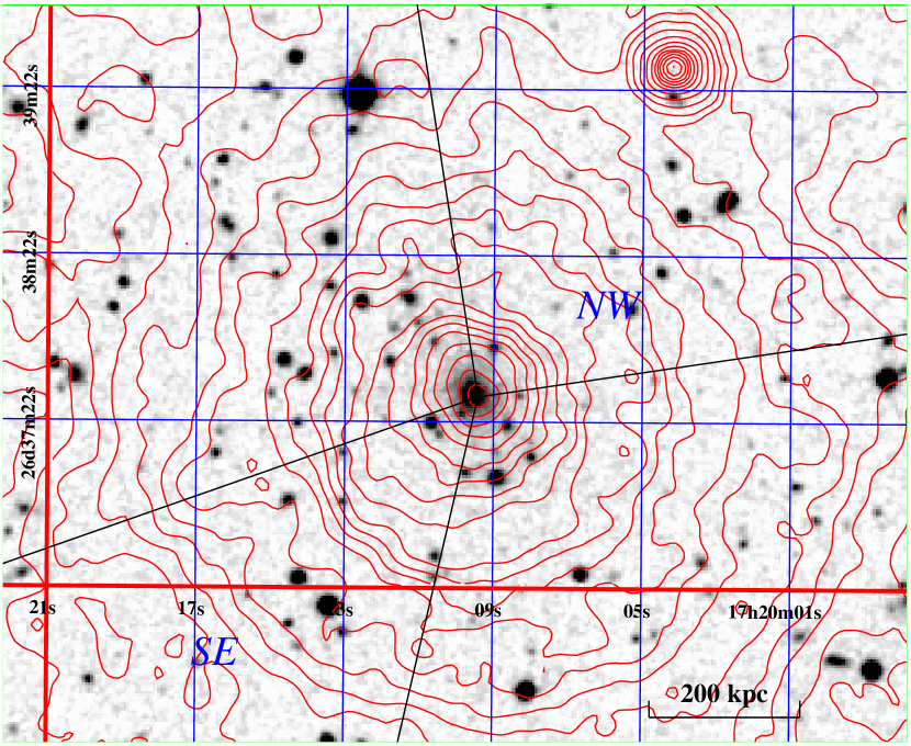
Figure 1: Digitized Sky Survey image with overlaid ACIS-I X-ray surface brightness contours (log-spaced by a factor of $\sqrt{2}$) in the 0.5-5 keV energy band after adaptive smoothing. The four straight lines starting from the X-ray brightness peak define the NW and the SE sectors whose angles are -80${}^{\circ}\!$  to 10${}^{\circ}\!$  and 109${}^{\circ}\!$  169${}^{\circ}\!$  respectively (the position angles are measured from North toward East). The central galaxy is nearly coincident with the X-ray peak.

To study the X-ray morphology of the cluster we generated an image with $1^{\prime\prime}\times 1^{\prime\prime}$ pixels from the events in the chips I0, I1, I2, and I3. We extracted the image in the 0.5-5 keV band to minimize the relative contribution of the cosmic background and thereby to maximize the signal-to-noise ratio. In Fig. 1 we overlay the ACIS-I, X-ray contours (after an adaptive smoothing of the image with a circular top hat filter with a minimum of 30 counts under the filter) on the DSS optical image. The X-ray brightness peak coincides with the optical center of the cluster central galaxy. Moreover the cluster appears spherically symmetric at large radii and the centroids of the X-ray surface brightness for $r\geq 100^{\prime\prime}$ are coincident within $4^{\prime\prime}$ with the X-ray peak. However, we cannot fit a simple $\beta$ model to the X-ray surface brightness. Even excluding the inner regions $r\leq 100-150h_{50}^{-1}$ kpc ($r\leq 27^{\prime\prime}-41^{\prime\prime}$) to account for an apparent cooling flow, we find a reduced $\chi^{2}>3$. The failure of the $\beta$ model is mainly due to data points at radii between $30^{\prime\prime}$ and $80^{\prime\prime}$.

The isointensity contours, in fact, show that the X-ray surface brightness has an azimuthally symmetric distribution at large radii ($r\geq 100^{\prime\prime}$) as well as at small radii ($r\leq 16^{\prime\prime}$). However, there is a steep gradient in the surface brightness followed by a plateau at $r=30^{\prime\prime}-50^{\prime\prime}$ to the North-West and a sharp edge at $r=70^{\prime\prime}$ to the South-East of the X-ray peak. The SE edge remains sharp within a sector of angular extent $\psi\approx\pm 30$${}^{\circ}\!$  before gradually vanishing.

2.2 Density Profiles

To derive the X-ray surface brightness profile across these two features, we divided the cluster into two sectors centered on the X-ray peak as shown in Fig. 1: North-West (NW) and South-East (SE). The sector angles are -80${}^{\circ}\!$  to 10${}^{\circ}\!$  and 109${}^{\circ}\!$ to 169${}^{\circ}\!$  for the NW and the SE regions respectively (the position angles are measured from North toward East). We extracted a surface brightness profile from these two sectors in circular regions as shown in Fig. 2a. The SE radial profile clearly shows a sharp edge at about $r=70^{\prime\prime}$, while the NW profile shows a plateau in the region between $r=30^{\prime\prime}-50^{\prime\prime}$. The radial derivative of the SE surface brightness profile is clearly discontinuous on a scale $\leq 10^{\prime\prime}$.

The NW brightness profile appears to be more continuous but it still could not be reasonably fitted (reduced $\chi^{2}>3$) with the sum of two beta models. This indicates that we are not observing the projection of two clusters/groups of galaxies along the line of sight. The particular shape of the brightness profiles, instead, may indicate discontinuities in the gas density profile.

TABLE 1

Model Fits

Sector	$\alpha$	$\beta$	$r_{c}$	$A_{jump}$	$r_{jump}$	$\xi$	$\chi^{2}/$
			(arcsec)		(arcsec)	(${}^{\circ}\!$)	d.o.f.
NW	$2.2$	$0.63$	$43$	$0.95$	$35$	—	48.6
	$\pm 0.02$	$\pm 0.02$	$\pm 2$	$\pm 0.06$	$\pm 3$		46
SE	$0.59$	$0.63$	$76$	$2.8$	$69$	12	39.5
	$\pm 0.07$	$\pm 0.04$	$\pm 11$	$\pm 0.2$	$\pm 2$	${}^{+23}_{-47}$	46

To quantify the discontinuities, we fit the brightness profiles with the density model defined in the Appendix. The idea behind the model is that we have two concentric regions with different radial gas density distributions. We assume that the gas density distribution is a spherically symmetric power-law for the innermost region ($r<r_{jump}$) and the usual $\beta-$model for the external one ($r>r_{jump}$). The density distribution is characterized by a discontinuity (“jump”) at $r_{jump}$ of amplitude $A_{jump}$. If $A_{jump}>1$, the projection in the plane of the sky of such a density model, produces an azimuthally symmetric brightness jump at $r_{jump}$.

As one can see from Fig. 1, the SE surface brightness jump is not azimuthally symmetric: it becomes less abrupt at some angle $\psi$. This may indicate that the discontinuity in the actual cluster gas distribution is smeared out at some angle.

To reproduce the observed SE brightness edge we modify the above density model introducing, at the interface of the internal and external regions, a boundary layer in which the gas density changes sharply but continuously from its value in the inner region to the value in the outer region. The thickness of this layer depends on the angle $\zeta$ from the axis of a chosen direction $\hat{\delta}$ (which will late define the direction of motion of the central gas cloud), being zero at the direction of the axis (where the density profile is truly discontinuous) and growing with $\zeta$. The physical significance of this model boundary layer will be touched upon in the Discussion. The particular functional shape of the density profile inside the layer (”matching function” defined in the Appendix) is not very important; we assume it is a power law determined by the layer thickness at each given direction. The dependence of the layer thickness on the angle $\zeta$ can be derived by matching the two-dimensional projection of the model to the image of the SE edge. Once this dependence is fixed (see Appendix), the radial brightness profile can be used to fit the remaining parameters of the model. We will see that the brightness profile even allows us to constrain the direction $\hat{\delta}$. In fact, the model is fit to the brightness profile with the free parameters being the inner power law slope, the core radius and the beta-model slope ($\beta$), the angle $\xi$ of the direction $\hat{\delta}$ with respect to the plane of the sky, and the radius and the amplitude of the jump. The best-fit values within their $90\%$ errors are reported in Table 1. The best-fit density model is shown in Fig. 2b and the corresponding brightness profile is overlaid as a histogram on the data points in Fig. 2a. We find that the best-fit density jump factor is $2.8$ while $\xi=12^{+23}_{-12}$ deg. Because the density model is symmetric for $\xi\rightarrow-\xi$, the direction $\hat{\delta}$ should lie within $35$${}^{\circ}\!$  of the plane of the sky.

As shown in the Appendix (Fig.7), the constraint $|\hat{\delta}|<35$${}^{\circ}\!$  comes from the fact that the density edge is present in a finite sector and would not be seen in projection if the angle were too large.

Unlike the SE sector, the NW sector is consistent with no density jump. Therefore, to fit the NW profile, we omit the matching function from the previous density model, by setting $L(\zeta)=0$. The best-fit density profile parameters (within their 90% errors) are given in Table 1 and the best-fit density model and the corresponding brightness profile are shown in Fig. 2b and Fig. 2a, respectively. Even if the NW density profile is consistent with no density jump, it shows an evident break in slope.

Finally, we notice that, while the density slopes at larger radii are similar for both the NW and the SE regions, the slopes of the inner regions are higher and lower for the NW and SE sectors, respectively.

We would like to remark that the SE and NW sectors have different density profiles in the regions we have modeled (beyond $r=16^{\prime\prime}$). Thus, our model cannot be extrapolated to smaller radii where the projected surface brightness distributions must ultimately agree at the center even though we accurately describe the gas density distribution at $r>16^{\prime\prime}$. We also ignored the gas temperature variation which represents a small correction ($\leq 0.5\%$) for the energy band that we are using.

The temperature structure of these features is discussed in §2.4 below.

2.3 Average Cluster Spectrum

Spectra were extracted in the 0.6-10 keV band in PI channels that correct for the gain difference between the different regions of the CCDs. The spectra where then grouped to have a minimum of 50 counts per bin and fitted using the XSPEC package (Arnaud 1996). Both the redistribution matrix (RMF) and the effective area file (ARF) for all the CCDs are position dependent. In our spectral analysis we computed position dependent RMFs and ARFs using the CIAO 1.1.3 package weighted them by the X-ray brightness over the corresponding image region. As a result of CTI, the quantum efficiency (QE) of the ACIS front-illuminated CCDs decreases far from the read-out at high energies. In building the position dependent ARFs we used a preliminary version of the QE non-uniformity calibration file that corrects for this effect assuming that all chip nodes behave identically (Vikhlinin 2000).

We extracted an overall spectrum for RXJ1720.1+2638  in the ACIS-I3 chip and fitted it with an absorbed single-temperature thermal model (Raymond & Smith 1977, 1992 revision). At the present stage of the Chandra  calibration the responses of the ACIS-I chips are uncertain below $E\approx 1$ keV. Thus we initially restricted our fit to the 1-10 keV energy band and we fixed the equivalent hydrogen column to the Galactic value ($N_{H}=4.06\times 10^{20}$cm^-2). The result of the fit is given in Table 2. The same table gives the result of our fit to the 1.5-10 keV spectrum extracted from the innermost $r=4.5^{\prime}$ region obtained with the ASCA-GIS detector fixing the equivalent hydrogen column to the Galactic value. We find that the ASCA  best fit temperature is in good agreement with the Chandra  result.

To test how the Chandra  low energy calibration uncertainties affect our results, we refitted the spectrum using the 0.6-10 keV energy band and $N_{H}$ as a free parameter. In this case we find that the temperature is in excellent agreement with our previous result (see Table 2) but the Chandra  data require a significantly higher equivalent hydrogen column. A similar calibration effect is seen in the Chandra  observation of the Coma cluster (OBSID=1113). We measured the temperatures by extracting 0.6-10 keV spectra in four rectangular regions on the ACIS-I3 chip parallel to the read out. We find that while the temperatures are within the errors of those measured by ASCA  (Donnelly et al. 1999) the measured absorption in each region is significantly higher than the Galactic value. We conclude that, at the present stage of the Chandra  calibration, to obtain a reliable temperature measurement it is prudent to restrict the analysis to energies 1-10 keV and fix the $N_{H}$ value. However, the measured temperature is not significantly affected when we use the entire 0.6-10 keV energy band with $N_{H}$ as a free parameter.

The total unabsorbed cluster flux in the 0.1-2.4 keV energy band, measured with ACIS, is $f_{X}=14.2\times 10^{-12}$ erg cm^-2 s^-1, which is consistent with the ROSAT  value ($f_{X}=14.3\times 10^{-12}$ erg cm^-2 s^-1, Ebeling et al. 1998). This flux corresponds to a luminosity of $L_{X}=16.5\times 10^{44}$ erg s^-1. From the $L_{X}-T$ relation in the 0.1-2.4 keV band (see e.g., Markevitch 1998), we find that the luminosity of RXJ1720.1+2638  is typical of a $T\approx 10$ keV cluster, a temperature much higher than what we measured. Below we investigate the spatial temperature structure which may be responsible for this discrepancy.

TABLE 2

Average Spectrum

	$T_{e}$	$N_{H}$	$Z$	$\chi^{2}/d.o.f$
	keV	$10^{20}$cm-2	$Z_{\odot}$
AXAF	$5.6\pm 0.5$	$4$	$0.44\pm 0.15$	144.4/122
AXAF	$5.2\pm 0.3$	$10\pm 1.1$	$0.58\pm 0.15$	185.6/154
ASCA	$5.6\pm 0.5$	$4$	$0.2\pm 0.15$	85.5/77

^a [1-10]  keV energy band
^b [0.6-10] keV energy band

2.4 Temperature Profile

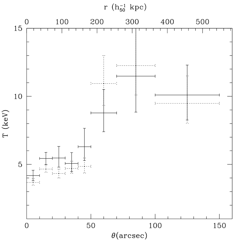
Figure 3: Temperature profile extracted from circular annuli centered on the X-ray peak (error bars $68\%$ confidence level).Dotted crosses: temperature profile obtained from the 0.6-10 keV band with $N_{H}$ as a free parameter. Solid crosses: temperature profile in the 1-10 keV band with $N_{H}$ fixed at the Galactic value.

We first derive a radial temperature profile of the entire cluster in eight annular regions centered on the X-ray peak. Following the procedure described in the previous section, we extracted the overall spectrum for each region. To quantify the corresponding uncertainties due to the low energy calibration problems, we fit the energy band from 1-10 keV with $N_{H}$ fixed at the Galactic value and the 0.6-10 keV band with $N_{H}$ free. In Fig. 3 we show the projected emission-weighted temperature profile. The solid and dotted crosses show the temperature profiles obtained from the 1-10 keV and 0.6-10 keV fits respectively; they are consistent within their statistical errors.

The temperature profile clearly shows the presence of at least two components: a more or less isothermal core region ($r<180h^{-1}_{50}$ kpc) with a temperature of $\approx 5$ keV, surrounded by a hotter, more extended region with $T\approx 10$  keV.

We notice that the temperature estimated from the temperature-luminosity relation is in agreement with the temperature measurement for the external region, suggesting that, on average, the properties of the external regions of the cluster are those of a hot, luminous cluster.

We also determined the 3-D temperature in the the innermost spherical $r=35^{\prime\prime}$ region by fitting the spectrum with a two temperature Raymond-Smith model, fixing the normalization and the temperature for the hotter component to those expected from spherical projection. We find that the true temperature of this central region is $\approx 3-4$ keV.

Because of the low energy calibration uncertainties it was not possible to confirm or exclude the spectroscopic signature of a cooling flow in the core of RXJ1720.1+2638. However, from the observed 3-D temperature and the gas density, we find the cooling time at the sharp borders of the core to be $t_{c}\approx 5\times 10^{9}$ Yr (see e.g., Sarazin 1988). This time is larger than the expected age of the cluster, thus it appears unlikely that the observed low temperature of the central region is the result of a cooling flow. Indeed, a rather constant temperature profile with a dip at the smallest radial bin suggests that cooling is significant only at that small radius.

To derive the detailed temperature structure across the brightness edges, we also extracted separate temperature profiles from the NW and the SE sectors, shown in Fig. 4. Due to the short exposure time, the statistical errors are rather large, but both profiles suggest a temperature rise as one moves outward across the brightness edges.

3 DISCUSSION

Density discontinuities similar to that seen in the SE sector of RXJ1720.1+2638  are theoretically expected in shock fronts in a gas flow (see Landau & Lifshitz 1959). However the temperature jump across the edge goes in the direction opposite to that expected for a shock front. Indeed, if we apply the Rankine-Hugoniot shock jump condition (see Landau & Lifshitz 1959,§§82-85), a factor of $\approx 2.6$ density jump with a post shock temperature of $\approx 3-4$ keV (the inner region of the SE edge), one would expect to find a $T\approx 1.5$ keV gas in front of the shock (on the side of the edge away from the cluster center) which is inconsistent with the much higher observed temperature (see Fig. 4).

Instead the observed sharpness and the temperature change of the SE edge are similar to those observed with Chandra  in two clusters with major mergers: A2142 (Markevitch et al. 2000b) and A3667 (Vikhlinin et al. 2000a). As suggested for those clusters, the most natural explanation is that the observed phenomenon is produced by the motion from NW to SE of a central, colder, denser body of gas through the hotter, cluster ICM. The X-ray edge is the surface of the contact discontinuity where the pressure in the dense core is in balance with the thermal plus ram pressure of the surrounding gas: the outer region of the moving gas cloud where the pressure was lower is stripped. The edge is sharp in the direction of motion, but is gradually destroyed by gas dynamic instabilities at an angle to that direction, as in A3667 (Vikhlinin et al. 2000a). Following Vikhlinin et al. (2000a), we estimate the speed of the dense cloud using the equations for flow past finite bodies (see Landau & Lifshitz 1959,§114):

$${\frac{p_{0}}{p_{1}}}=\left\{\begin{array}[]{*{2}{l}}\left(\frac{\gamma+1}{2}\right)^{(\gamma+1)/(\gamma-1)}\left[\gamma-\frac{\gamma-1}{2M_{1}^{2}}\right]^{-{1/(\gamma-1)}}M_{1}^{2};&M_{1}>1;\\ \left(1+\frac{\gamma-1}{2}M_{1}^{2}\right)^{\gamma/(\gamma-1)};&M_{1}\leq 1.\\ \end{array}\right.$$ (1)

Here $p_{0}$ is the pressure of the surrounding gas where the flow speed is zero (at the stagnation point immediately near the tip of the body). If we assume that the gas in the subclump does not expand, then the pressure $p_{0}$ is equal to the pressure just inside the edge. The parameters $p_{1}$ and $M_{1}$ are the the pressure of the incident gas and the Mach number (the ratio of the fluid velocity to the velocity of sound), respectively, calculated far from the body. Finally $\gamma$ is the ratio of the specific heats. Applying equation (1) to the measured pressure jump for the SE edge, we find $M_{1}=0.4^{+0.7}_{-0.4}$ which suggests that the central gas cloud moves subsonically (or at least not very supersonically) with respect to the surrounding gas.

Before discussing the nature of the moving core, we summarize the observational evidence:

1. the surface brightness is azimuthally symmetric at large radii and does not show the characteristic irregular structure typical of major mergers;

2. the external slopes ($\beta=0.63$) of the gas density are similar for the NW and the SE sectors, proving that the gas follows the same spherically symmetric potential at large radii;

3. the total cluster luminosity and the external temperature are consistent with the L-T relation (see §2.4);

4. the available DSS optical data, although not deep, exhibit only one central dominant galaxy and it is coincident with the X-ray surface brightness peak;

5. the velocity of the subclump is small compared to that of a point mass free-falling from infinity into the cluster center (assuming an isothermal cluster, $M_{1}\approx 2.7$; see e.g. Sarazin, 1988).

Below we discuss two possible evolutionary scenarios.

3.1 Major Merger

As suggested for A2142 and A3667, the most natural explanation for the presence of a moving subcluster is that RXJ1720.1+2638  is undergoing a merger. However, if this is the first or second passage of the subclump through the main cluster, then most of the above properties suggest that the merger direction is close to the line of sight. This is inconsistent with the presence of the SE surface brightness edge that clearly indicates that the merger direction should be within $35$${}^{\circ}\!$  of the plane of sky (see § 2.3).

On the other hand, if the merger direction is close to the plane of the sky, then the azimuthal symmetry and the low speed of the subclump require that the two merger objects, through damped oscillation, have already passed through each other several times and are now in the final stage before the cluster becomes fully relaxed. This raises the question of how the subclump could have survived such multiple core crossings without being disrupted by tidal forces. It is not clear to what extent subclumps of matter, that have already collapsed prior to infall into a larger cluster, can survive the infall. Analytic calculations suggest that, because of the tidal forces, groups of galaxies may not survive in a larger cluster environment for more than one crossing time (see e.g. González-casado, Mamon, & Salvador-Sole 1994). However recent, high resolution N-body simulations show that galaxy-like and group-like halos form and may survive even in the very central cluster region (Moore et al. 1999; Ghigna et al. 1999; Klypin et al. 1999). In any case it is clear that to survive tidal forces the central subclump must have a particularly compact, deep, gravitational potential that would have formed at high redshift.

3.2 Collapse of Two Density Perturbations

As noted above, the X-ray observations suggest that RXJ1720.1+2638  is composed of an extended hotter gas component with a spherically symmetric density distribution at radii $r>200-300h_{50}^{-1}$ kpc that hosts a moving, apparently thermally isolated, colder, compact ($r\approx 180h_{50}^{-1}$ kpc) object near its center.

An alternative to the merger hypothesis is that this cluster may be the result of the collapse of two different perturbations in the primordial density field on two different linear scales at nearly the same location in space. As the density field evolves, both perturbations start to collapse. The small scale perturbation collapses first and forms a central group of galaxies while the larger perturbation continues to evolve to form a more extended cluster potential. The central group of galaxies could have formed slightly offset from the center of the cluster and is now falling into or oscillating around the minimum of the potential well. This motion is responsible for the observed surface brightness discontinuity.

A possible problem with such a scenario is that we might expect some of the mass from the larger cluster perturbation to collapse onto the already virialized group by secondary infall of shells just beyond the group (e.g. Hoffman 1988). If the mass accretion of the group from secondary infall is too large, then it is plausible that the final stage of the evolution will result in just one single cluster potential, thus destroying the initial dual potential structure. However, we may expect that the effect of secondary infall is small enough that the group may maintain its own identity. In fact, a group is just a rescaled version of a galaxy (Moore et al. 1999) and N-body simulations of the formation and evolution of galactic halos in clusters clearly show that the mass of galactic halos that form inside a larger cluster-size perturbation stops evolving well before the cluster virializes (Okamoto & Habe 1999). We also note that dual potential structures have been suggested in previous works for several clusters (Thomas, Fabian, & Nulsen 1987; Nulsen & Böhringer 1995; Ikebe et al.1996). These authors suggest that the X-ray data for these clusters are consistent with two distinct components: a large-scale cluster component and a central compact component associated with the cD galaxy. This model then may represent a rescaled version of these previous suggestions.

Unlike a major merger, this last interpretation does not have a problem of tidal force disruption of the smaller central subclump. Indeed, the speed of the subclump may be subsonic just because its initial position lies well within the main cluster. This may indicate that we are observing the subclump’s first or second passage through the main cluster core and there has not been enough time for it to be tidally disrupted.

Our model suggests that the central group virialized earlier than the cluster itself. We can estimate the formation epoch of the group assuming that the external, higher gas temperature reflects the depth of the larger scale perturbation while the internal temperature is that of the originally colder central group, after some compression induced by the pressure of the cluster gas. Because the present pressure at the center of the group is much higher than the pressure of the cluster near the group, such compression cannot have been very significant.

Therefore, we simply assume that the observed internal temperature is that of the central group at the time it virialized. We can also estimate the gas mass associated with the central group assuming that the total gas mass is the sum of the gas masses inside the two hemispheres of radius $r_{jump}$ with density profiles given by the best-fit values in Table 1 for both NW and SE sectors. We find $M_{g}=8.8\times 10^{12}h_{50}^{-5/2}M_{\odot}$. Because the central region is an ellipsoid rather than a sphere, our calculation may overestimate the actual gas mass by not more than a factor $1/e^{2}$, where $e$ is the eccentricity. The eccentricity of the central region that we measured from the X-ray surface brightness appears to be $\leq 0.77$. Thus, we can safely constrain the total gas mass associated with the central group to be $M_{g}\approx 5-9\times 10^{12}h_{50}^{-5/2}M_{\odot}$.

Using the $M_{g}-T$ relation (see e.g. Mohr et al. 1999; Nevalainen, Markevitch, & Forman 2000; and references therein) and assuming that $z_{g}$ is the redshift at which the group virialized, we find that the measured gas mass corresponds to that of a group with a temperature of $T\approx(1-1.5)(1+z_{g})$ keV. In $\S 2.4$ we estimate the group 3-D temperature to be $T\approx 3-4$ keV. Thus, the latter equation allows us to constrain the group formation redshift to $1<z_{g}<3$. From the dissipationless uniform spherical collapse model (Peebles 1980) we know that the time $t_{c}$ at which a perturbation collapses and the time $t_{m}$ at which the perturbation reaches its maximum expansion are related as $t_{c}=2\times t_{m}$. If we assume that the larger scale perturbation collapsed just at the cluster redshift ($z=0.164$), then the same perturbation reached its turn around point at $z=0.85$. Thus, at the time when the group had already formed, the larger scale perturbation was still expanding with the Hubble flow and, hence, the central group was only weakly affected by its environment, a situation in accord with our model.

3.3 Hydrostatic Equilibrium at the Subclump Boundaries

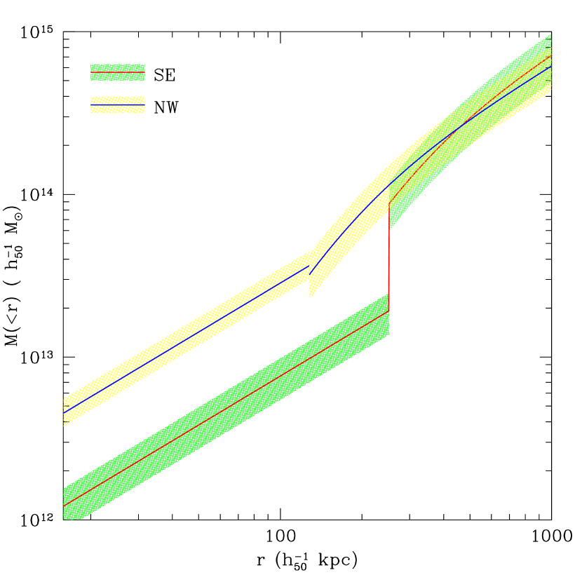
Figure 5: The integrated total gravitating mass distribution derived, under the assumption of hydrostatic equilibrium, from the SE and NW gas density properties, respectively.

Regardless of the origin of the central subcluster, it is interesting to consider its effect on the estimate of the total mass. For gas in hydrostatic equilibrium, the hydrostatic equation can be used to estimate the cluster mass inside a radius $r$ (see e.g., Bahcall & Sarazin 1977; Mathews 1978). In Fig. 5 we show the total mass profiles derived from the gas density properties of the SE and NW sectors, assuming hydrostatic equilibrium. We assume also that the gas temperature is constant just inside and outside the density breaks (below we discuss the effect of a possible temperature gradient in the central region). We use the temperature values from Fig. 4 for the external regions and the 3-D temperature within the group ($T=3.5\pm 0.5$ keV) for the internal region. The assumption of no temperature gradient on either side of the front is consistent with our data and is supported by analogy with A3667 where the data show a clear temperature discontinuity at the edge and no temperature gradient just inside and outside the edge. Moreover, for A3667 we know that, because the front width is 2-3 times smaller than the Coulomb mean free path (Vikhlinin et al. 2000a), the two gases at the edge are thermally isolated, which we may reasonably expect here as well.

Fig. 5 shows that the cluster mass determinations for the SE and NW sectors are in agreement (as they must be) only at radii larger than the SE edge. In particular, at the density jump for the SE sector, we find that, within the same radius, $M_{int}=(1.9\pm 0.6)\times 10^{13}h_{50}^{-1}M_{\odot}$ and $M_{ext}=(9.5\pm 3)\times 10^{13}h_{50}^{-1}M_{\odot}$ (the subscripts $int$ and $ext$ refer to the estimates from the data in the internal and external regions, respectively; errors are 68% confidence level). Even though the statistics are rather poor, the mass appears to be discontinuous, with the mass just inside the edge lower than the mass outside. This is obviously an unphysical result.

The discontinuity of the mass estimate comes from the fact that both the temperature and the density slope ($d\log n/d\log r$) decrease as one crosses the edge from the outside to the inside.

Possible explanations for the measured mass discontinuity are:

1. the temperature within the colder region is not constant;

2. the gas inside the cloud is not in hydrostatic equilibrium.

A positive temperature gradient is not excluded by the observed temperature profile (see e.g. Fig. 4). Such a gradient would act to increase the mass inside the edge, reducing the mass discrepancy. However, if we make a simple assumption that within the central core $T\propto r^{\gamma}$, to remove the mass discrepancy we need $\gamma\approx 2$. This implies that the temperature at $r=35^{{\prime\prime}}$ should be $\approx 1.7$ times smaller than the temperature at $r=45^{{\prime\prime}}$ which is clearly inconsistent with the observed temperature profile (see Fig. 3 and Fig. 4).

As for the hydrostatic assumption, we know that the subclump moves subsonically relative to the sound speed of the external gas where the temperature is $T\approx 10$ keV. However, the temperature of the subclump gas is $T\approx 3-4$ keV, which means that the speed of sound in the gas of the moving subclump is a factor $1.6-1.8$ lower than that in the external gas. Because of the uncertainties in the measured subclump speed, we cannot exclude a supersonic motion of the subclump relative to the sound speed in its own gas. If it is indeed supersonic, then the subcluster gas may not have sufficient time to react to any perturbations caused by the changing external ram pressure, for example, and therefore may not be in hydrostatic equilibrium. This may distort our mass estimate $M_{int}$.

Regardless of the physical mechanism responsible for the SE edge mass discrepancy, it is clear from Fig. 5 that any attempt to measure the total mass using the hydrostatic equation in circular annuli would result in a significant underestimate of the total cluster mass at small radii.

The linear scale of the central moving gas cloud is approximately equal to the core size for this cluster (see Table 1) and also to the radial distance where we expect to find strong lensing in clusters like RXJ1720.1+2638. Moreover, because the observed width of the discontinuities is $\leq 10^{{\prime\prime}}$, similar features may not have been revealed by previous X-ray missions and may, potentially be responsible for some of the discrepancy between the X-ray and the lensing mass determinations found in some systems (see e.g. Miralda-Escudé & Babul 1995; but Allen 1998; and reference therein).

4 CONCLUSION

We have presented the results of a short Chandra  observation of the cluster of galaxies RXJ1720.1+2638. The data indicate a remarkable surface brightness edge in the SE sector of the cluster consistent with a discontinuity in the density profile along that direction, and a plateau in the NW sector consistent with a break of the gas density profile. The edge and the break separate the colder inner region from the hotter external region. The structure of the SE edge is similar to the “cold fronts” observed by Chandra  in the merging clusters A2142 and A3667. We argue that such a discontinuity is produced by the subsonic motion from NW to SE of the central cold, group-size cloud of gas with respect to the cluster. Unlike A2142 and A3667, RXJ1720.1+2638  does not show the characteristic elongation and irregular structure typical of a major merger, and the optical data show only one central dominant galaxy coincident with the X-ray surface brightness peak. Moreover, the subclump speed appears to be small compared to that expected in the first passage of a subclump infalling from a large distance. We, therefore, propose a scenario in which RXJ1720.1+2638  is the result of the collapse of a group of galaxies followed by the collapse of a much larger, cluster-scale perturbation at nearly the same location in space. The available data are consistent with this scenario as well as with that of a final stage of a major merger before the cluster becomes fully relaxed.

We also showed that because of the motion of the central gas cloud, the hydrostatic equilibrium equation may underestimate the true cluster mass in the cluster core. Such a phenomenon may explain, in part, the discrepancy between the X-ray and the strong lensing mass determinations found in some systems.

Appendix A DENSITY MODEL

Below we define the gas density distribution $n_{0}$ that we use to fit the surface brightness profile at the SE edge. We consider a system of spherical coordinates oriented so that ($r,\theta=\pi/2,\varphi=0$) points along the line of sight toward us. We define a direction $\hat{\delta}$ that lies in a plane perpendicular to the plane of the sky at an angle $\xi$ with respect to the plane of the sky; this will be the axis of cylindrical symmetry of our model. The density distribution has three distinct regions (internal, boundary, and external):

$$n_{0}(r,\theta,\varphi)\propto\left\{\begin{array}[]{*{2}{l}}f_{int}(r),&r<r_{int}(\zeta),\\ &\\ f_{match}(r),&r_{int}(\zeta)<r<r_{ext}(\zeta),\\ &\\ f_{ext}(r),&r<r_{ext}(\zeta),\\ &\\ \end{array}\right.$$ (A1)

In the internal and external regions, the profile is:

$$\begin{array}[]{*{1}{l}}f_{int}(r)=A_{jump}\left({r/r_{jump}}\right)^{-\alpha},\\ f_{ext}(r)={\left(1+({r_{jump}/r_{c}})^{2}\right)^{3\beta/2}/{\left(1+({r/r_{c}})^{2}\right)^{3\beta/2}}}.\end{array}$$ (A2)

These are functions only of the radial distance $r$, and

$$\begin{array}[]{*{1}{l}}r_{int}(\zeta)=r_{jump}\exp(-L(\zeta)),\\ r_{ext}(\zeta)=r_{jump}\exp(L(\zeta)),\end{array}$$ (A3)

are functions only of the angle $\zeta$ from the direction $\hat{\delta}$: $\zeta(\theta,\varphi)=\sqrt{(\theta-{\pi/2})^{2}+(\varphi+\xi-{\pi/2})^{2}}$.

Along the direction $\hat{\delta}$, the width of the boundary layer ($r_{int}-r_{ext}$) is 0 and the density distributions $f_{int}(r)$ and $f_{ext}(r)$ are connected at $r=r_{jump}$ by a density discontinuity (jump) of amplitude $A_{jump}$. For $\zeta>0$, we define a simple “matching” function $f_{match}(r)$, which is a power-law that continuously connects $f_{int}(r_{int}(\zeta))$ with $f_{ext}(r_{ext}(\zeta))$:

$$f_{match}=f_{int}(r_{int})(r/r_{int})^{\nu},$$ (A4)

where

$$\nu=\frac{\log(f_{ext}(r_{ext}))-\log(f_{int}(r_{int}))}{2L(\zeta)}.$$ (A5)

The angular dependence of the width of the boundary layer is given by equations (A3) and

$$L(\zeta)=S(1-\exp{\left[-{(\zeta^{2}/(2\sigma^{2})}\right]}.$$ (A6)

The values $S$ and $\sigma$ can be chosen from a comparison of the model to the observed image. We generated a number of models and we found that $S=0.5$, $\sigma=40$${}^{\circ}\!$  is the best choice. After these two parameters are chosen from the image, the remaining parameters, such as the slopes of the density profiles, are derived from a fit to the brightness profile as described in § 2.2. Fig. 6 shows the corresponding synthesized image in the case $\xi=0$ ( $\hat{\delta}$ in the plane of the sky), and the best-fit values from Table 1.

This model appears particularly useful for estimating the angle of the symmetry axis $\hat{\delta}$ with respect to the plane of the sky. The shape and the sharpness of the surface brightness profile, in fact, are strong functions of this angle, as shown in Fig. 7. Indeed, as the direction $\hat{\delta}$ moves from the plane of the sky, the shape of the surface brightness becomes smother and the edge vanishes.

We also ran a number of simulations using different matching functions and we found that, as long as we maintain the condition that the model image is similar to the observed one, the important parameters of the density distribution are not significantly affected.

Figure 2: X-ray surface brightness and gas density model profiles across the density jumps. The left and the right panels refer to the SE and NW sectors respectively. Panels a) – X-ray surface brightness profiles across the density jumps. The errors are $1\sigma$. The histogram is the best-fit brightness model that corresponds to the gas density model shown in panels b). Panels b) – The best-fit gas density model for the X-ray surface brightness profile of panels a) (assuming spherical symmetry; see text).

Figure 4: Temperature profile extracted from circular annuli centered on the X-ray peak in the 1-10 keV band (error bar $68\%$). The left and the right panels refer to the SE and NW sectors respectively. The vertical dotted lines indicate the best-fit $r_{jump}$ values.

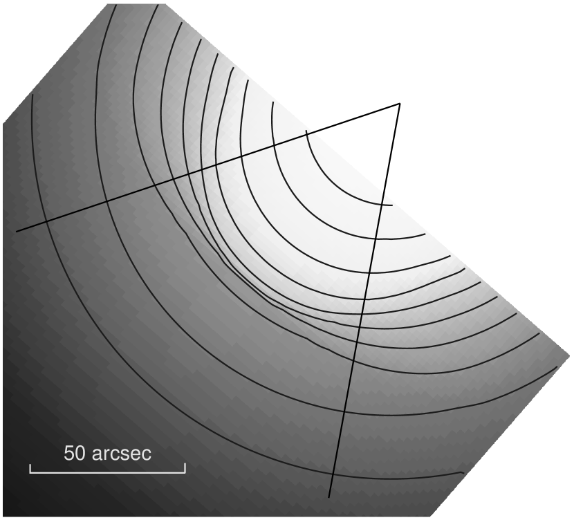
Figure 6: X-ray surface brightness image obtained by projecting the density model defined in the appendix on the plane of the sky.The contours are log-spaced by a factor of $\sqrt{2}$. Here $S=0.5$, $\sigma=40$${}^{\circ}\!$ , $\xi=0$${}^{\circ}\!$  ( $\hat{\delta}$ is in the plane of the sky), and the best-fit parameters are from Table 1. The two radial lines indicate a sector of angular extent $\psi=\pm 30$${}^{\circ}\!$.

Figure 7: Projected surface brightness profiles as a function of the direction $\hat{\delta}$. The density model parameters are the same as in Fig. 6. The solid, dotted, and dashed lines correspond to direction angles $\xi=12$${}^{\circ}\!$ , $\xi=40$${}^{\circ}\!$ , and $\xi=60$${}^{\circ}\!$ , respectively. The data points with error bars correspond to the observed SE X-ray surface brightness profile (see Fig. 2).

References

- (1)
- (2) Allen, S. W., 1998, MNRAS, 296, 392
- (3) Arnaud, K. A. 1996, ASP Conf. Ser. 101, Astronomical Data Analysis Software and Systems V, 5, 17
- (4) Reviews of Modern Astronomy, 8, 259
- (5) Bahcall, J. N., & Sarazin, C. L. 1977, ApJ, 213, L99
- (6) Crawford, C. S., Allen, S. W., Ebeling, H., Edge, A. C., & Fabian, A. C. 1999, MNRAS, 306, 857
- (7) Davis, M., Efstathiou, G., Frenk, C. S., & White, S. D. M. 1985, ApJ, 292, 371
- (8) Donnelly, R. H., Markevitch, M., Forman, W., Jones, C., Churazov, E., & Gilfanov, M. 1999, ApJ, 513, 690
- (9) Ebeling, H., Edge, A. C., Bohringer, H., Allen, S. W., Crawford, C. S., Fabian, A. C., Voges, W., & Huchra, J. P. 1998, MNRAS, 301, 881
- (10) Ghigna, S., Moore, B., Governato, F., Lake, G., Quinn, T., Stadel, J. 2000, ApJ, 544, 616
- (11) González-Casado, G., Mamon, G. A., & Salvador-Sole, E. 1994, ApJ, 433, L61
- (12) Harris, D. E., Dewdney, P. E., Costain, C. H., McHardy, I., & Willis, A. G. 1988, ApJ, 325, 610
- (13) Ikebe, Y. et al. 1996, Nature, 379, 427
- (14) Klypin, A., Gottlöber, S., Kravtsov, A. V., & Khokhlov, A. M. 1999, ApJ, 516, 530
- (15) Landau, L.D., & Lifshitz, E. M. 1959, Fluid Mechanics (London: Pergamon)
- (16) Markevitch, M. 1998, ApJ, 504, 27
- (17) Markevich, M. et al. 2000a, CXC memo (http://asc.harvard.edu/cal “ACIS”, “ACIS Background”)
- (18) Markevitch, M., Ponman, T. J., Nulsen, P. E. J., Bautz, M. W., Burke, D. J., David, L. P., Davis, D., Donnelly, R. H., Forman, W. R., Jones, C., Kaastra, J., Kellogg, E., Kim, D.-W., Kolodziejczak, J., Mazzotta, P., Pagliaro, A., Patel, S., VanSpeybroeck, L., Vikhlinin, A., Vrtilek, J., Wise, M., Zhao, P. 2000b, ApJ, 541, 542
- (19) Mathews, W. G. 1978, ApJ, 219, 413
- (20) Miralda-Escudé, J., Babul, A. 1995, ApJ, 449, 18
- (21) Moore, B., Ghigna, S., Governato, F., Lake, G., Quinn, T., Stadel, J., & Tozzi, P. 1999, ApJ, 524, L19
- (22) Nevalainen, J., Markevitch, M., & Forman, W. 2000, ApJ, 532, 694
- (23) Nulsen, P. E. J. & Böhringer, H. 1995, MNRAS, 274, 1093
- (24) Okamoto, T. & Habe, A. 1999, ApJ, 516, 591
- (25) Peebles, P.J. 1980, The Large Structure of the Universe, (Princeton: Princeton University Press)
- (26) Raymond, J. C., & Smith, B. W. 1977, ApJS, 35, 419
- (27) Sarazin, C. L. 1988, X-Ray Emission in Cluster of Galaxies (Cambridge: Cambridge Univ. Press)
- (28) Thomas, P. A., Fabian, A. C. & Nulsen, P. E. J. 1987, MNRAS, 228, 973
- (29) Vikhlinin, A. 2000, CXC memo
- (30) (http://asc.harvard.edu/cal/Links/Acis/acis/Cal_prods/qe/03_22_00/index.html)
- (31) Vikhlinin, A., Markevitch, M., Murray, S.S. 2000a, ApJ, in press (asro-ph/0008496)
- (32) Vikhlinin, A., Markevitch, M., Murray, S.S. 2000b, ApJ, submitted (astro-ph/0008499)
- (33) White, S.D.M. & Rees, M. 1987, MNRAS, 183,341
- (34)