The Pearson-Readhead Survey of Compact Extragalactic
Radio Sources From Space. I. The Images

M. L. Lister¹¹affiliation: Jet Propulsion Laboratory, California Institute of Technology, MS 238-332, 4800 Oak Grove Drive, Pasadena, CA 91109-8099 ²²affiliation: Current address: NRAO, 520 Edgemont Road, Charlottesville, VA 22903-2454 , S. J. Tingay¹¹affiliation: Jet Propulsion Laboratory, California Institute of Technology, MS 238-332, 4800 Oak Grove Drive, Pasadena, CA 91109-8099 ³³affiliation: Australia Telescope National Facility, P.O. Box 76, Epping, NSW 2121, Australia , D. W. Murphy¹¹affiliation: Jet Propulsion Laboratory, California Institute of Technology, MS 238-332, 4800 Oak Grove Drive, Pasadena, CA 91109-8099 , B. G. Piner¹¹affiliation: Jet Propulsion Laboratory, California Institute of Technology, MS 238-332, 4800 Oak Grove Drive, Pasadena, CA 91109-8099 ⁴⁴affiliation: Whittier College, Department of Physics, 13406 Philadelphia Street, Whittier, CA 90608 , D. L. Jones¹¹affiliation: Jet Propulsion Laboratory, California Institute of Technology, MS 238-332, 4800 Oak Grove Drive, Pasadena, CA 91109-8099 ,
R. A. Preston¹¹affiliation: Jet Propulsion Laboratory, California Institute of Technology, MS 238-332, 4800 Oak Grove Drive, Pasadena, CA 91109-8099 mlister@nrao.edu

Abstract

We present images from a space-VLBI survey using the facilities of the VLBI Space Observatory Programme (VSOP), drawing our sample from the well-studied Pearson-Readhead survey of extragalactic radio sources. Our survey has taken advantage of long space-VLBI baselines and large arrays of ground antennas, such as the Very Long Baseline Array and European VLBI Network, to obtain high resolution images of 27 active galactic nuclei, and to measure the core brightness temperatures of these sources more accurately than is possible from the ground. A detailed analysis of the source properties is given in accompanying papers. We have also performed an extensive series of simulations to investigate the errors in VSOP images caused by the relatively large holes in the $(u,v)$ plane when sources are observed near the orbit normal direction. We find that while the nominal dynamic range (defined as the ratio of map peak to off-source error) often exceeds 1000:1, the true dynamic range (map peak to on-source error) is only about 30:1 for relatively complex core-jet sources. For sources dominated by a strong point source, this value rises to approximately 100:1. We find the true dynamic range to be a relatively weak function of the difference in position angle (PA) between the jet PA and $(u,v)$ coverage major axis PA. For low signal-to-noise regions typically located down the jet away from the core, large errors can occur, causing spurious features in VSOP images that should be interpreted with caution.

galaxies : jets — galaxies : active — quasars : general — radio galaxies : continuum — techniques: high angular resolution — techniques : interferometric

^†^†slugcomment: Accepted for publication in the Astrophysical Journal

1 INTRODUCTION

Ground-based very long baseline interferometric (VLBI) surveys of the parsec-scale regions of active galactic nuclei (AGNs) have led to important insights into the nature of relativistic bulk outflows in compact radio sources. Here we present observational data from the first imaging survey of a complete sample of compact extragalactic radio sources made with space-VLBI. Our objects are selected from the well-studied Pearson-Readhead sample of AGNs, and are representative of some of the brightest, most compact AGNs in the sky.

Space-VLBI represents a logical step in the evolution of radio interferometry, and has the potential to provide the highest angular resolution images of any observing technique. Since our understanding of AGNs has historically been closely tied to resolution (e.g., the discovery of jets with connected interferometers, and relativistic bulk motions with VLBI), space-VLBI has an important role in AGN research.

The first successful space-VLBI experiments were accomplished in 1986 and 1987 using a TDRSS communications satellite (Levy et al., 1986; Linfield et al., 1989, 1990), and provided direct evidence for exceedingly compact emitting regions in extragalactic radio sources. In 1997, the first satellite dedicated to radio astronomical observations (HALCA) was launched by Japan’s Institute of Space and Astronautical Science, as part of the VLBI Space Observatory Programme (VSOP). HALCA’s highly elliptical orbit has an apogee height of 21,400 km, making it possible to directly image compact radio sources at 1.4 and 5 GHz with sub-milliarcsecond angular resolution, and to measure brightness temperatures in excess of $10^{12}$ K (Hirabayashi et al., 1998).

The images presented here are of the highest angular resolution ever achieved at 5 GHz, and reveal substantially more structural detail than previous ground VLBI studies of the Pearson-Readhead sample (e.g., Pearson & Readhead, 1981, 1988; Cawthorne et al., 1993). In §2 we describe our VSOP observations and data analysis methods, and present the images and basic data on our sample. We describe our model fitting technique in §2.2, and discuss the impact of incomplete $(u,v)$ plane coverage on space-VLBI images in §3. A full analysis of our space-VLBI data is presented in two companion papers (Tingay et al. 2001; Lister et al. 2001).

2 OBSERVATIONS AND DATA ANALYSIS

The Pearson-Readhead (PR) survey is a complete sample of 65 northern ( $\delta>+35^{o}$ ) AGNs with 5 GHz flux densities $>1.3$ Jy, and galactic latitude $|b|>10^{o}$ (Pearson & Readhead, 1988). In order to maximize the likelihood of detecting fringes to HALCA (at the $7\sigma$ level), we have selected as space-VLBI targets 31 PR objects that have flux densities $>0.4$ Jy on the longest Earth baselines ( $\sim 10,000$ km).

Observations of 27 of these objects were conducted with the HALCA orbiting antenna over the period 1997 August to 1999 April at a frequency of 5 GHz, in conjunction with telescopes from either the Very Long Baseline Array (VLBA), the European VLBI Network (EVN), or in some cases, both arrays. Four sources (0454+844, 0804+499, 0945+408, and 0954+658) were not observed due to scheduling constraints. HALCA was tracked typically between four and five hours per observation, synthesizing $(u,v)$ coverages with a maximum baseline of nearly 500 M $\lambda$ , or $~{}30,000$ km. A journal of our observations is given in Table 1.

Left circular polarization data from the ground antennas, or in the case of the orbiter, the spacecraft tracking station, were recorded on VLBA format tapes in two 16 MHz IFs and shipped to the VLBA correlator in Socorro for processing. The correlated data were amplitude-calibrated, fringe-fitted, and frequency-averaged in AIPS¹¹1AIPS and the VLBA are maintained by the National Radio Astronomy Observatory, which is operated by Associated Universities, Inc., under cooperative agreement with the National Science Foundation. before being exported to DIFMAP (Shepherd et al., 1994) for self-calibration, imaging and model-fitting.

Once imported into DIFMAP, the visibilities were edited and then coherently averaged over 30 second intervals. Due to its relatively small diameter (8 m) and poor antenna efficiency, the system equivalent flux density of HALCA is approximately 50 times worse than that of a typical VLBA antenna at 5 GHz. In order to give effectively equal weight to the ground-only and ground-space visibilities, we increased the weight of the HALCA antenna in self-calibration and subsequent model-fitting by a factor based on the relative number of ground-ground and space-ground visibilities and their respective baseline sensitivities. These factors are listed in Table 1.

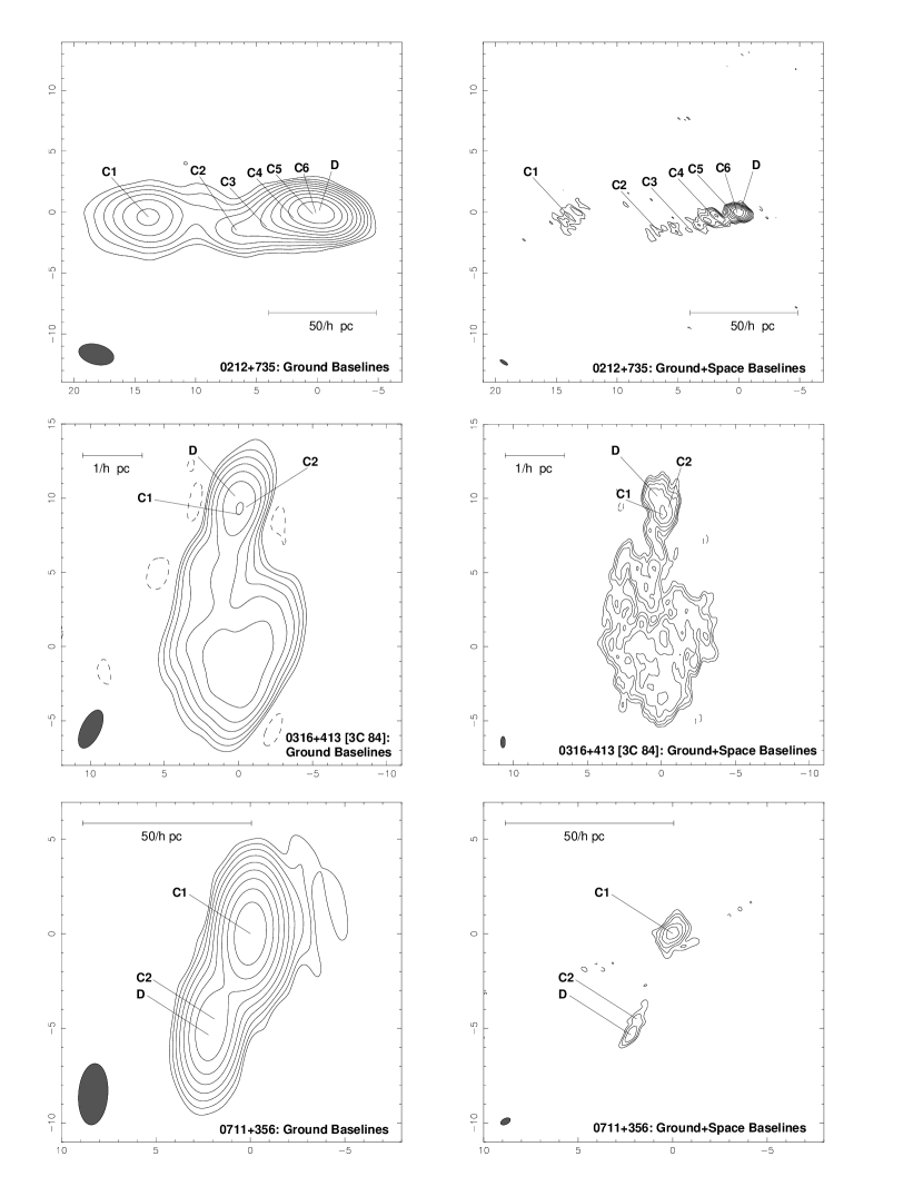
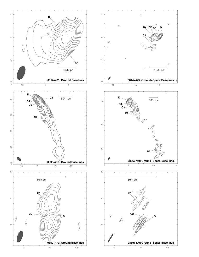
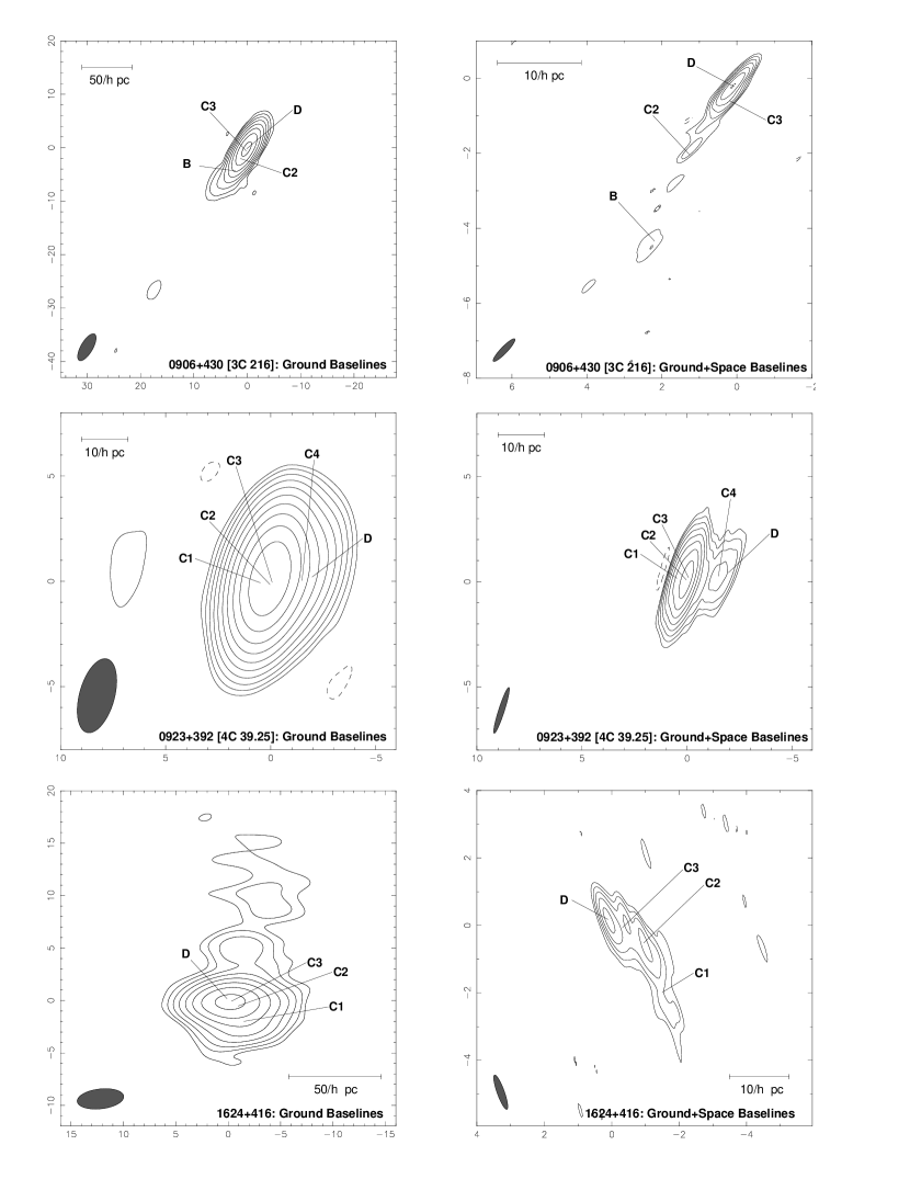
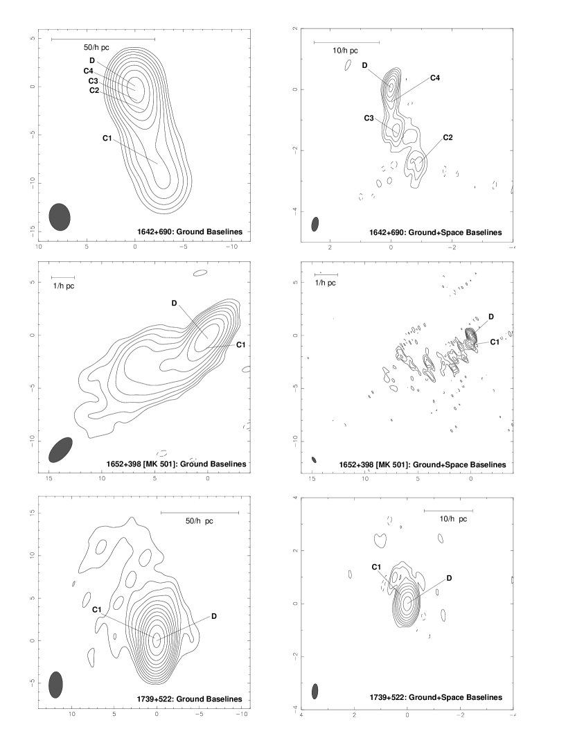
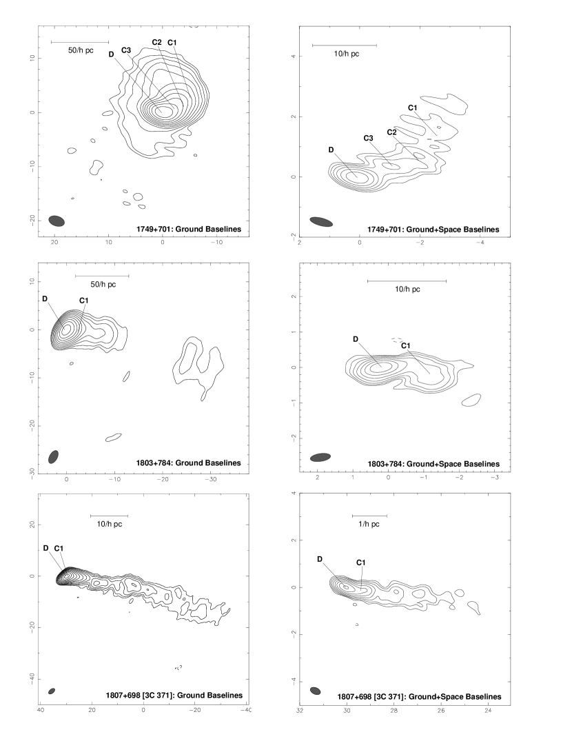
Following amplitude and phase self-calibration, we produced several images for each source using different visibility weighting schemes. The choice of weighting scheme has a large influence on space-VLBI images, due to the unequal numbers of ground-ground and ground-space visibilities, and the large differences in baseline noise level described above. Uniform weighting reduces the influence of the ground-ground visibilities on the image, which would normally dominate since they outnumber the space-ground visibilities. In the right-hand panels of Figures 1-9, we show uniformly-weighted images made using all available baselines. These images have no additional weighting by amplitude errors. In the left-hand panels, we show naturally-weighted images made using ground-ground visibilities only. We also include a representation of the restoring beam in the lower left corner of each image, and a bar showing the spatial scale. The latter is based on a standard Freidmann cosmology with zero cosmological constant, deceleration parameter $q_{o}=0.1$ , and Hubble constant $H_{o}=100\ h\ \rm km\ s^{-1}\ Mpc^{-1}$ . We will assume this model throughout this paper. The parameters of the restoring beam, the peak brightness, and the contour levels of each image are listed in Table 2.

In Table 3 we list the basic data on each source, including redshift, total amount of cleaned flux in the VLBI map, and an estimate of the total (single-dish) 4.8 GHz flux density at the epoch of the VSOP observation. The latter data were obtained by interpolating data from the University of Michigan monitoring program²²2http://www.astro.lsa.umich.edu/obs/radiotel/umrao.html, and have an approximate error of $\pm 0.1$ Jy.

2.1 Visibility Functions

The visibility function of a source represents the observed power measured on different spatial scales, with the long baselines representing small-scale structure, and vice-versa. In Figure 10 we plot the upper envelopes of the visibility amplitude distribution versus projected baseline length for the strongest and weakest sources, respectively. Instead of dropping smoothly to zero, the curves show a pronounced flattening at baselines greater than an earth diameter. This is indicative of strong, compact components that remain unresolved at the longest baselines. The brightness temperatures of these components and their implications for relativistic beaming models are discussed more fully by Tingay et al. (2001).

2.2 Component Model-fitting

We began our model-fitting analysis of each source with the core component, which is commonly believed to be associated with a flat-spectrum component located near the base of the jet. Wherever possible, we relied on previously published identifications to determine the position of the core. For sixteen sources the core (labeled “D” in Figures 1-9) was located at the end of the jet, and was also the brightest component in the 5 GHz image. In the case of nine sources, the component at the end of the jet was the brightest component in images at higher frequencies, but not at 5 GHz. The core component identifications for the two radio galaxies in our sample are somewhat uncertain, as their jet structure may not be one-sided. For 3C 84 (0316+413), we arbitrarily assigned the core position to the northernmost component of the jet, while for 2021+614, we used the core identification of Tschager et al. (2000).

We first removed the set of point source clean components used to fit the core from the clean component model and replaced them with an elliptical Gaussian described by 6 free parameters. We then fit the Gaussian in the $(u,v)$ plane using the MODELFIT task in DIFMAP, which uses a linear least squares fit to the amplitude and phase to find the best fit model. For all our fits, we adjusted the visibility weights used in the least squares calculation, such that the ground antennas and the space antenna contributed equally to the reduced chi-squared statistic. We interspersed runs of MODELFIT with phase self-calibration, to ensure that the reduced chi-squared was minimized to find the best fit models. The parameters of our core-component fits are given in Table 4.

After fitting the core, we removed the clean components associated with various other isolated features and model-fit them with elliptical Gaussians. In order to avoid introducing new nomenclature for individual components, we have used existing names from the literature wherever possible. These are given in Table 5, along with the parameters of our fits. We caution that these fits may not be robust, especially in regions where there is continuous jet emission. Indeed, some features (e.g., the southernmost component of 2021+614) were too complex to be represented by simple Gaussians, and were not model-fitted.

We determined errors on the parameters of the core-component models using the DIFWRAP package (Lovell, 1998), a graphical interface to DIFMAP which fixes given parameters of the models at different values which are perturbations on the best-fit values, and allows all other parameters to vary freely to re-minimize the reduced chi-squared. In this way it is possible to determine how far from the best-fit value a given parameter can be forced before the model no longer fits the $(u,v)$ plane data, defining the error on that parameter.

For each source, we first determined whether the core component could be fit with an unresolved point source (i.e., a delta-function component). If a point source did not fit the visibilities within the amplitude errors, we then tried one-dimensional (zero-axial ratio) components of various lengths and position angles (PAs). If none of these provided a good fit, we varied the parameters of the best-fit model as described above to determine the range of possible brightness temperature that still fit the visibility data. In two cases (0923+392 and 2021+614), the cores were too weak with respect to the extended emission to determine a best fit range of brightness temperature.

The components in our sample could have also been fit using the surface brightness distributions of optically thin or optically thick spheroids, instead of Gaussian profiles. This is due to the fact that their Fourier transforms are virtually identical in the $(u,v)$ plane out to the point at which the flux density is $50\%$ of the zero baseline flux density (Pearson, 1995). Since we do not generally observe past this point for the core components in our sources, we have adopted Gaussian surface brightness distributions. To convert the observed brightness temperature assuming a Gaussian component to an optically thin or optically thick sphere, corrective factors of 0.67 and 0.56 respectively, should be applied.

We find that the sizes of our fitted components generally increase exponentially with distance down the jet. In Figure 11 we present a log-log plot of fitted component area ( $\Omega$ ) in square parsecs against projected distance from the core component ( $r$ ) in parsecs. A strong trend is present, with a linear correlation coefficient of 0.42, and a significance level of $99.985\%$ . The dashed line represents a linear regression through the points (in log space) of the form $\log{\Omega}=(1.4\pm 0.1)\log{r}+(0.07\pm 0.1)$ . The fit considering quasars alone is $\log{\Omega}=(1.1\pm 0.2)\log{r}+(0.5\pm 0.2)$ , and for BL Lacertae objects alone it is $\log{\Omega}=(1.5\pm 0.2)\log{r}-(0.2\pm 0.2)$ . These fitted slopes are all significantly less than two, which is the value for a conical jet of constant opening angle. Considering the fact that the projected distances in Fig. 11 are likely to be severely foreshortened due to small viewing angles (see Paper II), the trend indicates that the jets are still in a state of expansion and are undergoing collimation at distances of several hundred parsecs from the core.

2.3 Influence of $(u,v)$ Coverage on Model-fits

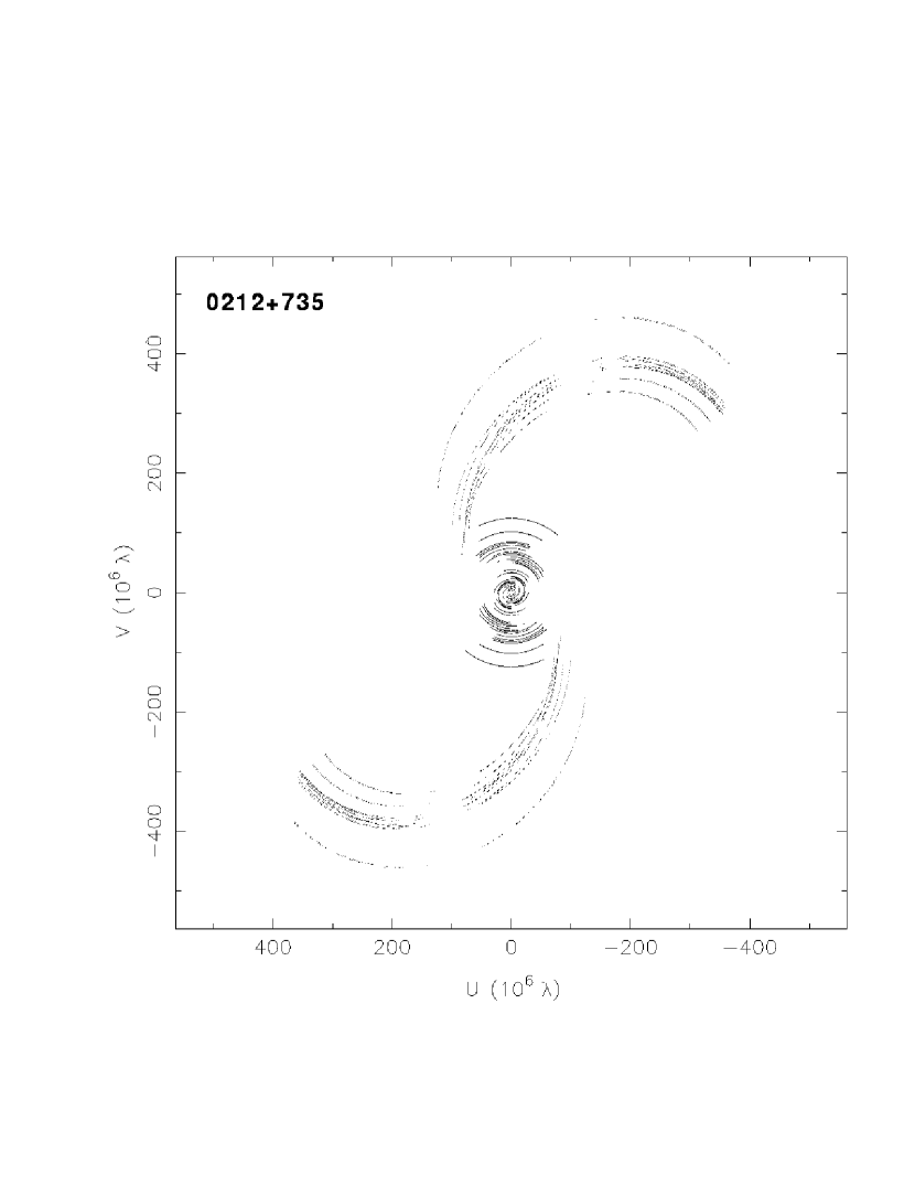
The $(u,v)$ coverages of most of our space-VLBI observations are highly elongated, due to the elliptical orbit of the HALCA satellite (Figure 12). As a result, the angular extent of the jets and components in our sample are much better constrained along one direction. We have examined the possible effects of this unequal $(u,v)$ plane sampling on our core component model-fits by inter-comparing the position angles of the fitted Gaussian component major axis, the position angle of the restoring beam, and the position angle of the parsec-scale jet.

We find that the major axis position angle of the fitted core component is strongly correlated with that of the beam and $(u,v)$ coverage, and therefore does not likely reflect an intrinsic property of the source. For those sources whose cores could be fit with a zero-axial ratio (ZAR) component, the $(u,v)$ coverage is generally perpendicular to the jet direction, and the fitted major axis of the ZAR component is aligned with the jet. This suggests that there are two or more closely spaced components in the core region that are separated by much less than a beam width. Since they cannot be resolved, the visibility data can be fit with a long, narrow (ZAR) component. In this case, the upper limit on the brightness temperature is unconstrained.

3 EFFECTS OF INCOMPLETE $(U,V)$ PLANE COVERAGE ON SPACE-VLBI IMAGES

Most of the space-VLBI observations of our sample were scheduled when the source lay close to the orbit normal. Under these conditions the maximum possible spatial resolution can be achieved, at the cost of creating relatively large holes in the $(u,v)$ plane aperture coverage. This is due to the the fact that the HALCA spacecraft has a highly elliptical orbit with an apogee height of 21,400 km, which greatly exceeds an Earth diameter. The effects of $(u,v)$ plane under-sampling are well-documented for ground-based inteferometric arrays (e.g., Perley, 1989), but relatively little work has been published for the case of space-VLBI. Here we discuss the effects of $(u,v)$ -holes on the quality of our space-VLBI images, and how the resulting imaging errors depend on the source’s jet position angle relative the position angle of the major axis of the $(u,v)$ coverage.

3.1 Example Simulations

We have addressed these issues by performing extensive image simulations using several different source models. These simulations have thermal amplitude and phases errors added to them at the same level as is present in the real data. Thus, the RMS noise-level on simulated HALCA baselines is about 7 times higher than on the simulated ground-only baselines. The simulated data were imaged using the same DIFMAP package that was used to reduce our actual space-VLBI data. For the purposes of this discussion we will consider the image artifacts which are present in 5 GHz images for the following source models, all of which are composed of Gaussian components:

1) A complex core-jet source which has a total flux density of 2.7 Jy. We will refer to this model as cj-complex;

2) A simple core-jet source, which has a 1 Jy, 10¹² K core with axial ratio unity and a 1 Jy, 10¹¹ K ‘jet’ with axial ratio 1/3 whose centroid is located at a distance of 1.21 milliarcseconds away from the core. The major axis of this component measures 1.21 milliarcseconds, and is aligned with the core-jet direction. We will refer to this model as cj-simple;

3) A 1 Jy, 10¹² K circular Gaussian;

4) A 1 Jy, 10¹⁴ K circular Gaussian. This source is completely unresolved for VSOP 5 GHz observations and can be used to determined the image artifacts in unresolved point sources. It is therefore a useful point of reference when examining the artifacts in more complex sources.

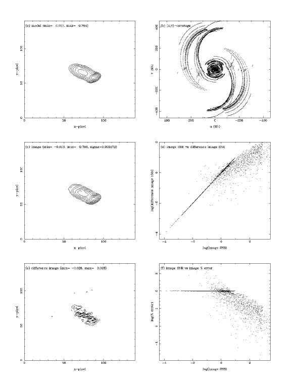
In Figures 13 and 14 we show two simulations we have performed using the cj-complex and cj-simple models respectively. We use the same $(u,v)$ coverage in both cases (panel b), which has a major axis PA of 0^∘. Both jets have a PA of 60^∘.

Panels (a), (c), and (d) show the model, simulated image, and difference image, respectively, all convolved with an identical beam that corresponds to uniform weighting of the visibility data. The difference image is simply defined as the difference between the the simulated image and the model. The difference images reveal a common error feature seen in the imaging of core-jet sources, in the form of a sinusoidal ripple that runs along the length of the jet. This feature is the result of a well-known instability of the CLEAN algorithm, and has modulations that tend to correspond with the spacing of holes in the $(u,v)$ plane (Cornwell, 1983). In our simulations, this error feature is so prominent that it can cause visible artifacts to occur in the jet that may easily be over-interpreted as discrete components. It is important, therefore, to exercise caution in the interpretation of relatively weak features in VSOP images.

A good example of this can be found in the model in Figure 13, in which panel (a) shows a rather smooth jet. The simulated VSOP image, on the other hand, shows a series of discrete components which run down the jet (panel c). In panels (d) and (f) the difference map signal-to-noise ratio (SNR) at each pixel and the percentage error in the simulated are shown as a function of the simulated image SNR. The SNRs quoted here use a reference noise level determined far away from the source structure. From these two panels we can see how the imaging errors decrease as the map SNR increases. For high SNR points ( $>$ 100) the image error is typically less than $10\%$ . However, for intermediate SNR points ( $10<{\rm SNR}<100$ ) the percentage error can almost be 100%, so caution must be exercised in over-interpreting data with this SNR.

3.2 Dynamic Range

A common method of quantifying image errors is to take the maximum in the image divided by the off-source RMS noise level ( $DR_{\rm RMS}$ ), which is sometimes referred to as the dynamic range of an image. For example, the simulated images shown in Figures 13 and 14 have $DR_{\rm RMS}$ values of 1600:1 and 2800:1 respectively. However, as our simulations show, this is not the true dynamic range in the image as the on-source errors are much larger than the off-source errors. We define here a new dynamic range, called $DR_{\rm diff}$ which is the maximum in the image divided by the maximum value (whether positive or negative) in the difference image. Using this definition, $DR_{\rm diff}$ has values of 34:1 and 28:1 for the images in Figures 13 and 14. Consequently the true dynamic ranges ( $DR_{\rm diff}$ ) of these images are a factor of $\sim 50$ worse compared to the dynamic range using the off-source noise level ( $DR_{\rm RMS}$ ). For comparison, the images made using the single $10^{12}$ K and $10^{14}$ K Gaussian component models, have values of $DR_{\rm RMS}$ of 3000:1 and 4000:1, and $DR_{\rm diff}$ of 48:1 and 130:0, respectively. Thus, we see a general trend of increasing image fidelity as the source structure becomes simpler (i.e., $DR_{\rm diff}$ decreases). However, even in the limit of a unresolved point source, the value of the true dynamic range is limited to approximately $100:1$ .

3.3 Effects of Jet Position Angle on Image Dynamic Range

One might expect that the dynamic range that we can obtain on a given observation of a source should depend on the difference between a source’s jet PA and the PA of the $(u,v)$ coverage major axis ( $\Delta PA$ ). For $\Delta PA$ =0^∘ we get the highest resolution along the jet and for $\Delta PA$ = 90^∘ we get the highest resolution perpendicular to the jet. Thus, the ability of the sinusoidal image error to develop could depend on the value of $\Delta PA$ . Consequently, certain alignments of jet position angle with respect to the $(u,v)$ coverage might be more reliable than those of a different $\Delta PA$ . We have investigated this phenomenon by conducting a series of simulations using the same $(u,v)$ coverage as shown in Figures 13 and 14 but for different values of the jet PA in the model sources cj-complex and cj-simple. In Figures 15 and 16 we plot how both $DR_{\rm RMS}$ and $DR_{\rm diff}$ vary as a function of the jet PA while keeping the PA of the major axis of the $(u,v)$ coverage fixed. As can be seen, $DR_{\rm RMS}$ is almost independent of $\Delta PA$ and $DR_{\rm diff}$ is only a relatively weak function of this position angle difference.

4 SUMMARY

We have presented data from the first imaging survey of a complete sample of compact extragalactic radio sources made with space-VLBI. These data represent the highest angular resolution images ever obtained for these objects at 5 GHz, and provide important information regarding the structure of AGN jets on parsec scales. In particular, we have found an exponential trend of increasing component size with distance down the jet, which indicates that these jets are still undergoing expansion on scales of several hundred parsecs. We have also detected a pronounced flattening in the visibility functions of our sources, which is indicative of strong, compact components that remain unresolved at the longest space-Earth baselines. We discuss the implications of this trend and the other general properties of our sample in two companion papers (Tingay et al. 2001; Lister et al. 2001).

We have performed an extensive series of simulations to investigate the image errors in VSOP images caused by the relatively large holes in the $(u,v)$ plane when sources are observed near the orbit normal direction. We find that while the nominal dynamic range ( $DR_{\rm RMS}$ ) often exceeds 1000:1, the true dynamic range ( $DR_{\rm diff}$ ) is about 30:1 for relatively complex core-jet sources. For sources dominated by a strong point source, this value rises to approximately 100:1. The true dynamic range is also found to be a relatively weak function of the difference in position angle between the jet PA and $(u,v)$ coverage major axis PA. For high SNR regions in the image (SNR $>$ 100) the error on individual pixels is typically less than $10\%$ . However, for low SNR regions typically located down the jet away from the core, large errors can occur and spurious features can be seen. Caution should therefore be exercised when interpreting regions of low SNR in VSOP images.

We gratefully acknowledge the VSOP Project, which is led by the Japanese Institute of Space and Astronautical Science in cooperation with many organizations and radio telescopes around the world. This research has made use of data from the University of Michigan Radio Astronomy Observatory, which is supported by the National Science Foundation and by funds from the University of Michigan. This work was undertaken in part at the Jet Propulsion Laboratory, California Institute of Technology, under contract with the National Aeronautics and Space Administration. SJT acknowledges support through an NRC/NASA-JPL Research Associateship.

References

Cawthorne et al. (1993) Cawthorne, T. V., Wardle, J. F. C., Roberts, D. H., & Gabuzda, D. C. 1993, ApJ, 416, 519
Cornwell (1983) Cornwell, T. J. 1983, A&A, 121, 281
Hirabayashi et al. (1998) Hirabayashi, H., et al. 1998, Science, 281, 1825
Hummel et al. (1997) Hummel, C. A., Krichbaum, T. P., Witzel, A., Wuellner, K. H., Steffen, W., Alef, W. & Fey, A. 1997, A&A, 324, 857
Kameno et al. (2000) Kameno, S., Shen, Z., Inoue, M., Fujisawa, K. & Wajima, K. 2000, in Astrophysical Phenomena Revealed by Space VLBI, eds. H. Hirabayashi, P. G. Edwards, & D. W. Murphy (Institute of Space and Astronautical Science: Sagamihara), 63
Klare et al. (2000) Klare, J., Zensus, J. A., Ros, E. & Lobanov, A. P. 2000, in Astrophysical Phenomena Revealed by Space VLBI, eds. H. Hirabayashi, P. G. Edwards, & D. W. Murphy (Institute of Space and Astronautical Science: Sagamihara), 21
Levy et al. (1986) Levy, G. S. et al. 1986, Science, 234, 187
Linfield et al. (1989) Linfield, R. P., et al. 1989, ApJ, 336, 1105
Linfield et al. (1990) Linfield, R. P., et al. 1990, ApJ, 358, 350
Lister & Smith (2000) Lister, M. L. & Smith, P. S. 2000, ApJ, 541, 66
Lister et al. (2001) Lister, M. L., Tingay, S. J., & Preston, R. A. 2001, ApJ, in press (Paper II)
Lovell (1998) Lovell, J. E. J. 1998, in Astrophysical Phenomena Revealed by Space VLBI, eds. H. Hirabayashi, P. G. Edwards, & D. W. Murphy (Institute of Space and Astronautical Science: Sagamihara), 301
Murphy et al. (2000) Murphy, D. W., Preston, R. A., Polatidis, A., Conway, J. E., Hirabayashi, H., Murata, Y. & Kobayashi, H. 2000, in Astrophysical Phenomena Revealed by Space VLBI, eds. H. Hirabayashi, P. G. Edwards, & D. W. Murphy (Institute of Space and Astronautical Science: Sagamihara), 47
Paragi et al. (2000) Paragi, Z., Frey, S., Fejes, I., Porcas, R. W., Schilizzi, R. T. & Venturi, T. 2000, in Astrophysical Phenomena Revealed by Space VLBI, eds. H. Hirabayashi, P. G. Edwards, & D. W. Murphy (Institute of Space and Astronautical Science: Sagamihara), 59
Pearson & Readhead (1981) Pearson, T. J., & Readhead, A. C. S. 1981, ApJ, 248, 61
Pearson & Readhead (1988) Pearson, T. J., & Readhead, A. C. S. 1988, ApJ, 328, 114
Pearson (1995) Pearson, T. J. 1995, in Very Long Baseline Interferometry and the VLBA, eds. J. A. Zensus, P. J. Diamond, & P. J. Napier (PASP: San Francisco), 267
Perley (1989) Perley, R. A. 1989, in Synthesis Imaging in Radio Astronomy, eds. R. A. Perley, F. R. Schwab, & A. H. Bridle (PASP: San Francisco), 287
Shepherd et al. (1994) Shepherd, M. C., Pearson, T. J., & Taylor, G. B. 1994, BAAS, 26, 987
Tingay et al. (2001) Tingay, S. J., et al. 2001, ApJ, in press
Tschager et al. (2000) Tschager, W., Schilizzi, R. T., Röttgering, H. J. A., Snellen, I. A. G. & Miley, G. K. 2000, A&A, 360, 887

Table 1: Journal of Observations

IAU	Other	Observing	Ground	Observing	Integration	HALCA
Name	Name	Date	Antenna Array	Freq.[GHz]	Time [h]^a^aApproximate ground integration time on source. Values in parentheses indicate integration time that included the HALCA spacecraft.	Weight^b^bWeighting assigned to the HALCA antenna during self-calibration and model-fitting (ground visibilities had a nominal weighting factor of unity).
0016+731	$\cdots$	1998 Mar 2	VLBA+U	4.81	10 (3)	1156
0133+476	OC 457	1999 Aug 16	VLBA	4.81	5 (4.5)	274
0153+744	$\cdots$	1998 Aug 18	VLBA $-$ Br,Sc,La	4.81	6 (5.5)	187
0212+735	$\cdots$	1997 Sep 5	VLBA $-$ Sc	4.97	8 (4.5)	415
0316+413	3C 84	1998 Aug 25	VLBA+Y	4.97	6 (5)	538
0711+356	OI 318	1999 Apr 9	VLBA	4.81	6 (4)	324
0814+425	OJ 425	1999 Apr 24	VLBA	4.81	6 (5)	289
0836+710	4C 71.07	1997 Oct 7	VLBA	4.97	5.5 (3.5)	390
0859+470	4C 47.29	1999 Feb 14	JEGNMTWO	4.97	6.5 (1)	1460
0906+430	3C 216	1999 Feb 14	JEGNMTW	4.97	5.5 (3)	399
0923+392	4C 39.25	1997 Oct 23	VLBA+Y	4.97	2.5 (2)	847
1624+416	4C 41.32	1998 Feb 7	VLBA $-$ Mk	4.81	4 (1.5)	347
1633+382	4C 38.41	1998 Aug 4	VLBA+Y	4.81	5.5 (4)	531
1637+574	OS 562	1998 Apr 21	VLBA $-$ Sc,Ov,Kp	4.81	6.5 (4.5)	280
1641+399	3C 345	1998 Jul 28	VLBA+EY	4.81	4.5 (3.5)	674
1642+690	4C 69.21	1998 May 31	JEGNMWS	4.97	6.5 (4.5)	225
1652+398	MK 501	1998 Apr 7	VLBA+E	4.81	5 (3.5)	370
1739+522	4C 51.37	1998 Jun 14	VLBA	4.81	6.5 (4)	391
1749+701	$\cdots$	1999 Jun 1	VLBA	4.81	8 (5)	406
1803+784	$\cdots$	1997 Oct 17	VLBA	4.97	6 (4)	370
1807+698	3C 371	1998 Mar 11	VLBA	4.81	6 (5)	349
1823+568	4C 56.27	1998 May 31	JEGNMO	4.97	4.5 (3.5)	542
1828+487	3C 380	1998 Jul 4	VLBA+E	4.81	6 (4)	584
1928+738	4C 73.18	1997 Aug 22	VLBA+E	4.97	5.5 (4.5)	482
1954+513	OV 591	1997 Nov 10	EGNMWO	4.97	12 (4)	777
2021+614	OW 637	1997 Nov 7	VLBA+ENMO	4.97	5.5 (4.5)	575
2200+420	BL Lac	1997 Dec 8	VLBA	4.97	6.5 (5)	315

Note. — Antenna abbreviations: Br = Brewster, E = Effelsberg, G = Green Bank, J=Jodrell Bank, Kp = Kitt Peak, La = Los Alamos, M = Medicina, N = Noto, O = Onsala, Ov = Owens Valley, S = Sheshan, Sc = Saint Croix, T = Torun, U = Usuda, W = Westerbork, Y = Phased Very Large Array.

Table 2: Summary of Image parameters

Source	Baselines	Beam	PA	Peak	Contour levels
(1)	(2)	(3)	(4)	(5)	(6)
0016+731	Ground	1.37 x 2.02	$-18$	0.450	$-0.06$ , …, 61.44
	All	0.38 x 0.77	$-76$	0.216	$-1.5$ , …, 96
0133+476	Ground	1.72 x 4.09	3	1.795	$-0.1$ , …, 51.2
	All	0.23 x 0.61	$-29$	1.340	$-0.5$ , …, 64
0153+744	Ground	1.03 x 2.10	$-30$	0.295	$-1$ , …, 64
	All	0.36 x 0.52	$-36$	0.070	$-4$ , …, 64
0212+735	Ground	1.65 x 2.94	76	2.357	$-0.1$ , …, 51.2
	All	0.24 x 0.67	58	0.786	$-0.4$ , …, 51.2
0316+413	Ground	1.27 x 2.80	$-26$	1.944	$-1.5$ , …, 96
	All	0.31 x 0.77	0	0.375	$-2.5$ , …, 80
0711+356	Ground	1.56 x 3.26	$-4$	0.707	$-0.2$ , …, 51.2
	All	0.31 x 0.55	$-63$	0.189	$-4$ , …, 64
0814+425	Ground	1.55 x 3.11	$-21$	0.589	$-0.2$ , …, 51.2
	All	0.26 x 0.82	$-42$	0.437	$-0.75$ , …, 96
0836+710	Ground	1.57 x 2.88	51	0.844	$-0.25$ , …, 64
	All	0.22 x 0.62	$-36$	0.372	$-1.25$ , …, 80
0859+470	Ground	0.93 x 2.20	$-19$	0.533	$-0.5$ , …, 64
	All	0.20 x 1.88	$-32$	0.264	$-5$ , …, 80
0906+430	Ground	2.23 x 5.70	$-30$	0.610	$-0.65$ , …, 83.2
	All	0.17 x 0.82	$-44$	0.381	$-1.5$ , …, 96
0923+392	Ground	1.67 x 3.63	$-16$	9.490	$-0.1$ , …, 51.2
	All	0.28 x 2.28	$-18$	4.092	$-0.5$ , …, 64
1624+416	Ground	1.90 x 4.46	$-83$	0.419	$-0.6$ , …, 76.8
	All	0.22 x 1.08	20	0.126	$-4.5$ , …, 72
1633+382	Ground	1.37 x 3.44	5	0.893	$-0.1$ , …, 51.2, 95
	All	0.25 x 0.66	$-27$	0.397	$-0.75$ , …, 96
1637+574	Ground	1.55 x 2.97	$-28$	0.506	$-0.25$ , …, 64
	All	0.26 x 0.52	4	0.226	$-1.5$ , …, 96
1641+399	Ground	0.62 x 3.15	$-8$	1.877	$-0.2$ , …, 51.2
	All	0.24 x 0.64	$-14$	0.940	$-1$ , …, 64
1642+690	Ground	2.17 x 2.83	8	0.625	$-0.25$ , …, 64
	All	0.22 x 0.47	$-10$	0.372	$-1.25$ , …, 80
1652+398	Ground	1.40 x 2.93	$-42$	0.509	$-0.4$ , …, 51.2
	All	0.25 x 0.62	$31$	0.325	$-1$ , …, 64
1739+522	Ground	1.62 x 3.11	$-2$	1.814	$-0.04$ , …, 81.92
	All	0.22 x 0.58	$-4$	0.918	$-0.5$ , …, 64
1749+701	Ground	1.83 x 2.98	72	0.312	$-0.05$ , …, 51.2
	All	0.25 x 0.77	75	0.169	$-1.75$ , …, 56
1803+784	Ground	1.61 x 2.95	$-29$	1.539	$-0.125$ , …, 64
	All	0.22 x 0.58	$-82$	0.928	$-0.8$ , …, 51.2
1807+698	Ground	1.61 x 2.87	$-50$	0.567	$-0.07$ , …, 71.68
	All	0.28 x 0.46	66	0.320	$-0.1$ , …, 51.2
1823+568	Ground	1.66 x 2.51	$-6$	0.817	$-0.3$ , …, 76.8
	All	0.25 x 0.68	16	0.536	$-0.75$ , …, 96
1828+487	Ground	0.95 x 1.67	$-40$	0.631	$-0.28$ , …, 71.68
	All	0.27 x 0.62	$-9$	0.379	$-0.9$ , …, 57.6
1928+738	Ground	0.76 x 1.59	23	1.311	$-0.3$ , …, 76.8
	All	0.40 x 0.54	$-42$	0.918	$-0.4$ , …, 51.2
1954+513	Ground	1.30 x 2.54	$-3$	0.600	$-0.2$ , …, 51.2
	All	0.25 x 0.48	$-34$	0.228	$-4$ , …, 64
2021+614	Ground	0.99 x 1.47	66	1.112	$-0.4$ , …, 51.2
	All	0.23 x 0.44	$-51$	0.401	$-1.2$ , …, 76.8
2200+420	Ground	1.57 x 3.05	$-24$	2.265	$-0.55$ , …, 70.4
	All	0.22 x 0.46	$-27$	1.239	$-1$ , …, 64

Note. — Columns are as follows: (1) Source name; (2) VLBI baselines used in image; (3) FWHM dimensions of Gaussian restoring beam, in milliarcseconds; (4) Position angle of restoring beam, in degrees; (5) Peak intensity of image [ $\rm Jy\ beam^{-1}$ ]; (6) Minimum and maximum contour levels, expressed as a percentage of peak intensity (intermediate contours are separated by factors of two).

Table 3: Source Properties

IAU	Other	Opt.		$S_{VLBI}$	$S_{tot}$
Name	Name	Id.	z	[Jy]	[Jy]
(1)	(2)	(3)	(4)	(5)	(6)
0016+731	$\cdots$	Q	1.781	0.581	0.8
0133+476	OC 457	Q	0.859	1.985	2.0
0153+744	$\cdots$	Q	2.338	1.090	1.1
0212+735	$\cdots$	Q	2.367	3.045	3.0
0316+413	3C 84	RG	0.017	17.494	22.2
0711+356	OI 318	Q	1.620	1.030	1.0
0814+425	OJ 425	BL	0.245	0.836	1.0
0836+710	4C 71.07	Q	2.180	1.762	2.2
0859+470	4C 47.29	Q	1.462	0.974	1.3
0906+430	3C 216	Q	0.670	0.684	1.6
0923+392	4C 39.25	Q	0.699	10.968	11.0
1624+416	4C 41.32	Q	2.550	0.668	0.9
1633+382	4C 38.41	Q	1.807	1.889	2.4
1637+574	OS 562	Q	0.749	0.703	0.9
1641+399	3C 345	Q	0.595	5.971	8.2
1642+690	4C 69.21	Q	0.751	0.878	1.2
1652+398	MK 501	BL	0.033	0.977	1.7
1739+522	4C 51.37	Q	1.381	1.933	2.2
1749+701	$\cdots$	BL	0.770	0.504	0.6
1803+784	$\cdots$	BL	0.680	2.040	2.2
1807+698	3C 371	BL	0.050	0.880	1.6
1823+568	4C 56.27	BL	0.663	1.047	1.6
1828+487	3C 380	Q	0.692	1.957	5.3
1928+738	4C 73.18	Q	0.302	3.324	3.7
1954+513	OV 591	Q	1.223	0.848	1.4
2021+614	OW 637	RG	0.228	2.664	2.8
2200+420	BL Lac	BL	0.069	4.069	4.4

Note. — Columns are as follows: (1) IAU Name; (2) Alternate name; (3) Optical identification, where Q = quasar, BL = BL Lacertae object, RG = radio galaxy; (4) Redshift; (5) Total 5 GHz cleaned flux density in VLBI image in Janskys; (6) Single dish 5 GHz flux density at VLBI observation epoch in Janskys, estimated from the University of Michigan light curve.

Table 4: Core Component Properties

Source	S	Maj.	Axial	PA	Fit	$T_{b}$
Name	[Jy]	axis	ratio	[deg.]	Type	$[/10^{12}\;\rm K]$
(1)	(2)	(3)	(4)	(5)	(6)	(7)
0016+731	0.118	0.53	0.45	$-$ 64	ZAR	$0.05^{+\inf}_{-0.03}$
0133+476	1.554	0.17	0.70	$-$ 6	ZAR	$3.9^{+\inf}_{-1.0}$
0153+744	0.352	1.17	0.40	$-$ 86	Res	$0.034^{+0.002}_{-0.01}$
0212+735	1.206	0.54	0.72	71	Res	$0.28^{+0.06}_{-0.03}$
0316+413	1.556	1.17	0.87	62	Res	$0.066^{+0.01}_{-0.02}$
0711+356	0.078	0.46	0.19	$-$ 36	ZAR	$0.10^{+\inf}_{-0.07}$
0814+425	0.448	0.09	0.53	$-$ 66	U	$5.4^{+\inf}_{-4.5}$
0836+710	0.603	0.28	0.46	49	ZAR	$0.83^{+\inf}_{-0.4}$
0859+470	0.447	0.85	0.16	$-$ 31	Res	$0.19^{+0.05}_{-0.05}$
0906+430	0.483	0.43	0.15	$-$ 34	Res	$0.86^{+0.8}_{-0.2}$
0923+392	0.267	1.01	0.34	$-$ 21	n/a^a^aComponent too weak to determine errors in model fit parameters.	$0.038$
1624+416	0.152	0.37	0.29	31	U	$0.20^{+\inf}_{-0.1}$
1633+382	0.443	0.15	0.71	$-$ 43	Res	$1.46^{+0.4}_{-0.2}$
1637+574	0.241	0.13	0.24	27	U	$3.13^{+\inf}_{-0.3}$
1641+399	0.811	0.40	0.63	$-$ 26	Res	$0.42^{+0.05}_{-0.01}$
1642+690	0.396	0.19	0.14	$-$ 22	ZAR	$3.87^{+\inf}_{-1.6}$
1652+398	0.450	0.24	0.87	32	Res	$0.47^{+0.4}_{-0.1}$
1739+522	1.745	0.33	0.88	$-$ 29	Res	$0.96^{+0.03}_{-0.03}$
1749+701	0.264	0.32	0.52	$-$ 50	ZAR	$0.26^{+\inf}_{-0.06}$
1803+784	1.374	0.29	0.63	88	Res	$1.28^{+0.6}_{-0.2}$
1807+698	0.387	0.28	0.29	71	ZAR	$0.90^{+1.1}_{-0.3}$
1823+568	0.791	0.60	0.20	16	Res	$0.54^{+0.1}_{-0.1}$
1828+487	0.510	0.42	0.12	$-32$	ZAR	$1.3^{+\inf}_{-0.5}$
1928+738	0.416	0.35	0.34	$-$ 21	ZAR	$0.49^{+\inf}_{-0.4}$
1954+513	0.313	0.40	0.23	$-$ 38	ZAR	$0.42^{+\inf}_{-0.1}$
2021+614	0.078	0.70	0.40	60	n/a^a^aComponent too weak to determine errors in model fit parameters.	$0.02$
2200+420	1.552	0.42	0.44	10	Res	$0.99^{+0.3}_{-0.2}$

Note. — Columns are as follows: (1) Source name; (2) Fitted 5 GHz flux density in Janskys; (3) Major axis of fitted Gaussian (FWHM) in milliarcseconds; (4) Axial ratio of component; (5) Position angle of component’s major axis; (6) Visibility data consistent within errors with: U = unresolved component; ZAR = component having zero-axial ratio; Res = component that is resolved on longest space baselines; (7) Brightness temperature of best component fit in units of $10^{12}K$ , with range of possible values that fit the visibility data.

Table 5: Jet Component Properties

Cpt.	$r$	$\theta$	S	Maj.	Axial	PA	log $T_{b}$
Name	[mas]	[deg.]	[Jy]	Axis	Ratio	[deg.]	[K]	Ref.
(1)	(2)	(3)	(4)	(5)	(6)	(7)	(8)	[9]
0016+731
C2	0.65	130	0.254	0.72	0.37	83	10.9	$\cdots$
C1	0.89	137	0.183	0.95	0.35	-64	10.5	$\cdots$
0133+476
C3	0.63	-31	0.221	0.89	0.16	0	11.0	$\cdots$
C2	1.44	-32	0.102	0.88	0.44	-64	10.2	$\cdots$
C1	3.75	-45	0.078	3.95	0.73	-44	8.6	$\cdots$
0153+744
B	10.16	157	0.592	1.91	0.58	-62	10.2	1
0212+735
C6	0.34	124	0.880	0.32	0.37	-7	12.1	$\cdots$
C5	0.60	117	0.347	0.42	0.00	-22	$\cdots$	$\cdots$
C4	2.21	106	0.347	1.68	0.45	88	10.1	$\cdots$
C3	4.55	107	0.047	1.70	0.29	89	9.4	$\cdots$
C2	7.00	103	0.050	1.55	0.41	-52	9.4	$\cdots$
C1	14.06	92	0.179	2.40	0.68	-53	9.4	$\cdots$
0316+413
C2	1.07	-134	0.501	0.96	0.36	21	10.9	$\cdots$
C1	1.30	-164	1.109	0.84	0.67	43	11.1	$\cdots$
0711+356
C2	0.90	-20	0.061	0.61	0.79	-45	10.0	$\cdots$
C1	5.80	-23	0.764	0.83	0.76	-53	10.9	$\cdots$
0814+425
C4	0.36	100	0.064	0.27	0.22	-31	11.3	$\cdots$
C3	1.05	87	0.140	0.51	0.79	-18	10.6	$\cdots$
C2	1.40	84	0.104	0.44	0.58	-56	10.7	$\cdots$
C1	2.27	140	0.047	2.10	0.44	8	9.1	$\cdots$
0836+710
C4	0.40	-132	0.097	0.17	0.18	79	11.9	$\cdots$
C3	1.29	-138	0.143	0.61	0.47	-30	10.6	$\cdots$
C2	2.68	-143	0.204	0.52	0.46	-20	10.9	$\cdots$
C1	11.57	-148	0.178	1.65	0.76	-0	9.6	$\cdots$
0859+470
C2	1.73	-9	0.366	1.82	0.74	-43	9.9	$\cdots$
C1	4.26	6	0.161	7.07	0.16	-10	9.0	$\cdots$
0906+430
C3	0.40	167	0.075	0.22	0.32	-45	11.4	$\cdots$
C2	2.16	147	0.050	1.78	0.13	-51	9.8	2
B	4.63	153	0.035	0.85	0.24	-81	10.0	2
0923+392
C4	0.51	110	0.263	1.69	0.21	-16	10.4	$\cdots$
C3	1.92	97	2.670	1.29	0.75	48	11.1	$\cdots$
C2	2.04	100	6.536	0.43	0.68	74	12.4	$\cdots$
C1	2.48	96	1.259	0.51	0.48	-31	11.7	$\cdots$
1624+416
C3	0.49	-119	0.084	0.86	0.32	4	10.3	$\cdots$
C2	1.26	-124	0.147	0.93	0.26	44	10.5	$\cdots$
C1	2.69	-143	0.114	2.57	0.54	32	9.2	$\cdots$
1633+382
C5	0.50	-78	0.270	0.47	0.15	-59	11.6	$\cdots$
C4	1.02	-75	0.442	1.20	0.26	-34	10.8	$\cdots$
A	1.91	-86	0.599	0.84	0.47	-29	11.0	3
C2	3.00	-88	0.046	0.54	0.56	-6	10.2	$\cdots$
C1	4.06	-73	0.035	1.60	0.11	-25	9.8	$\cdots$
1637+574
C2	0.97	-157	0.303	0.49	0.55	4	11.1	$\cdots$
C1	2.90	-160	0.098	1.14	0.72	49	9.7	$\cdots$
1641+399
C9	0.64	-122	1.891	0.39	0.74	49	11.9	4
C8	1.22	-102	1.569	0.40	0.92	49	11.8	4
C7	2.33	-101	0.607	0.63	0.86	-86	11.0	4
1642+690
C4	0.48	-178	0.086	0.28	0.54	16	11.0	$\cdots$
C3	1.52	-172	0.143	0.51	0.53	11	10.7	$\cdots$
C2	2.64	-159	0.107	0.40	0.58	-1	10.7	$\cdots$
C1	8.39	-164	0.051	1.97	0.36	-88	9.3	$\cdots$
1652+398
C1	0.89	168	0.067	0.49	0.26	63	10.8	$\cdots$
1739+522
C1	0.41	38	0.078	0.48	0.26	-12	10.8	$\cdots$
1749+701
C3	1.23	-72	0.082	0.95	0.35	82	10.1	$\cdots$
C2	2.12	-74	0.034	0.84	0.52	31	9.7	$\cdots$
C1	2.99	-62	0.033	1.02	0.63	3	9.4	$\cdots$
1803+784
C1	1.38	-98	0.413	0.65	0.82	50	10.8	$\cdots$
1807+698
C1	0.66	-102	0.231	0.74	0.28	-85	10.9	$\cdots$
1823+568
C3	1.24	-157	0.123	0.60	0.23	42	10.9	$\cdots$
C2	3.25	-165	0.060	1.88	0.14	1	9.8	$\cdots$
C1	7.39	-163	0.024	0.58	0.69	41	9.7	$\cdots$
1828+487
C2	3.28	-28	0.170	0.60	0.73	18	10.5	$\cdots$
A	9.26	-31	0.165	0.69	0.74	-87	10.4	5
1928+738
C5	0.67	149	1.292	0.43	0.42	-14	11.9	6
C4	1.95	159	0.429	0.60	0.61	7	11.0	6
C3	2.31	173	0.622	0.80	0.46	-22	11.0	$\cdots$
C2	3.68	160	0.190	1.34	0.42	-4	10.1	6
C1	5.22	164	0.051	1.06	0.38	-79	9.8	6
1954+513
C1	0.64	-56	0.348	0.43	0.37	-27	11.4	$\cdots$
2021+614
B	3.89	34	0.639	0.71	0.58	-47	11.0	7
C3	4.28	33	0.143	0.36	0.78	73	10.8	$\cdots$
C2	4.74	34	0.136	0.94	0.24	-41	10.5	$\cdots$
A	6.77	46	0.101	1.32	0.28	-61	10.0	7
2200+420
C3	0.88	-171	0.323	0.55	0.47	14	11.1	$\cdots$
C2	1.35	-160	0.805	0.43	0.96	83	11.3	$\cdots$
C1	2.43	-169	0.929	1.59	0.50	11	10.6	$\cdots$

Note. — Columns are as follows: (1) Component name; (2) Distance from core in milliarcseconds; (3) Position angle with respect to core; (4) Flux density in Jy; (5) Major axis of fitted component in milliarcseconds; (6) Axial ratio of fitted component; (7) Position angle of component’s major axis; (8) log of Gaussian brightness temperature in K; (9) Reference for component identifications: (1) Hummel et al. 1997; (2) Paragi et al. 2000; (3) Lister & Smith 2000; (4) Klare et al. 2000; (5) Kameno et al. 2000; (6) Murphy et al. 2000; (7) Tschager et al. 2000.