Radiative transfer in molecular lines

Abstract

The highly convergent iterative methods developed by Trujillo Bueno and Fabiani Bendicho (1995) for radiative transfer (RT) applications are generalized to spherical symmetry with velocity fields. These RT methods are based on Jacobi, Gauss-Seidel (GS), and SOR iteration and they form the basis of a new NLTE multilevel transfer code for atomic and molecular lines. The benchmark tests carried out so far are presented and discussed. The main aim is to develop a number of powerful RT tools for the theoretical interpretation of molecular spectra.

1 Introduction

Atomic line emission has been extensively used for tracing the physical conditions in many astrophysical plasmas. The relatively high energy difference between the atomic energy levels makes this diagnostic tool a suitable one for tracing the physical conditions in warm and hot media. But cool plamas are not well traced by atomic lines because the thermal energy is not high enough to populate the upper levels of the transitions. Fortunately, FIRST will allow us to study molecular line emission in greater detail. Molecules have very rich spectra, arising from transitions between the electronic, vibrational and rotational levels. Their spectra cover the spectral range from radio to optical wavelengths, depending on the type of transition. One has to include very complicated molecular systems to be able to model the observations and an extensive forward RT modeling effort is frequently needed. With this motivation in mind, we are developing a radiative transfer code based on the fast iterative methods developed by [*]tru95 for Cartesian coordinates. Our first step was to generalize these methods to spherical symmetry with velocity fields. This new RT tool will help us in the interpretation of different kinds of observations, including ro–vibrational bands in circumstellar envelopes of C-rich or O-rich evolved stars, rotational lines in molecular clouds, molecular emission from the Sun, maser emission and many others. Another interesting application would be the modeling of maser polarization.

2 The state of the art and our approach

The radiative transfer problem requires the self-consistent solution of the rate equations for the populations of the molecular levels and the radiative transfer equation. This set of equations describes a nonlinear and nonlocal problem. Iterative methods are therefore needed. Since [*]ber79, most of the radiative transfer tools used in molecular radiative transfer have been based on Monte Carlo techniques for the solution of the radiative transfer equation and on the $\Lambda$-iteration for the iterative solution of the non-LTE problem. The Monte Carlo technique is very powerful for its ability to cope with complicated geometries, but it has a major drawback: its instrinsic random noise. There have been many efforts to reduce the noise, but it is always present (see, for example, [Bernes1979]). On the other hand, the $\Lambda$-iteration scheme is very easy to implement, but is only useful for optically thin problems. Recently, Accelerated Lambda Iteration (ALI) methods have been applied to molecular radiative transfer. ALI is a method that requires not much more computational time per iteration than the $\Lambda$-iteration, but it has a better convergence behavior for optically thick problems. It has been extensively used in stellar and solar astrophysics and has recently been combined with Monte Carlo techniques for molecular RT ([Hogerheijde & van der Tak2000]).

Our approach is based on the iterative methods developed by [*]tru95, which themselves are based on the Gauss–Seidel scheme and applied to Cartesian coordinates in 1D, 2D and 3D, either with or without polarization. They allow the solution of the radiative transfer problem with the same computational time per iteration as ALI, but with an order-of-magnitude improvement in the number of iterations. The short-characteristics technique ([Kunasz & Auer1988]) has been chosen as the formal solver. This has facilitated the implementation of the scheme in a very efficient way (see [Trujillo Bueno & Fabiani Bendicho1995]). We have generalized these methods to spherical symmetry with velocity fields. The problem is still one dimensional because the physical variables have only radial dependence, but angular information has to be achieved more precisely than for a plane–parallel atmosphere in order to take account of curvature effects. This angular information is obtained by means of solving the RT equation through the impact parameters, as is usually done. The velocity fields are treated in the observer’s frame. In Fig. (1) we show a schematic representation of the difference between the ALI-based and the GS-based iterations. With ALI, when the radiation field is obtained at all the points of the atmosphere, the statistical equilibrium equations for the molecular population can be solved. On the other hand, the main idea behind the GS-based methods is the fact that when the radiation field is known at one point in the atmosphere, one can write the statistical equilibrium equations for this point and do the level population correction. When solving the RT equation to get the radiation field at the next point, we have to take into account that the population in the previous point has been improved. This scheme, coded in an efficient way with the aid of the short-characteristics formal solver, can lead to a high improvement in the total number of iterations, while the time per iteration is virtually the same as with ALI.

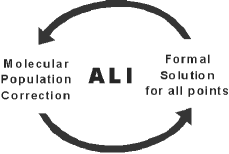
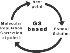
Figure 1: Scheme showing the differences between the ALI iterative method and the GS-based method. The figure is explained in the text.

3 Illustrative examples

In order to verify that our code is giving reliable results, we have chosen several benchmark problems whose results have already been published.

3.1 Bernes’s CO cloud

Let us begin with the CO cloud model used by [*]ber79 to introduce his Monte Carlo code. The problem consists in a constant-density ($n_{{\rm H}_{2}}=2\times 10^{3}$ cm^-3), constant-temperature ($T=20$ K), 1 pc radius infalling cloud with a maximum velocity of 1 km s^-1 at the external parts and sampled at 40 radial shells. The CO abundance is $5\times 10^{-5}$ and the cloud is illuminated by the cosmic microwave background radiation (CMBR) at a temperature of 2.7 K. The CO molecule with the first six rotational levels is used, taking into account that the same collisional rates used by Bernes in his calculation have to be used to get similar results. In Fig. (2) we show the excitation temperature for the transitions $J=1\rightarrow 0$ and $J=2\rightarrow 1$ through the cloud. We show the results obtained with our code and that obtained by Bernes using his Monte Carlo technique. The intrinsic noise of the Monte Carlo scheme can clearly be appreciated in the figures.

Figure 2: Excitation temperature for the $J=1\rightarrow 0$ and $J=2\rightarrow 1$ rotational transitions of CO in the Bernes’ cloud. Comparison between the our results and those of Bernes (1979) are plotted.

3.2 Leiden benchmark test

A number of useful test cases became available after the 1999 workshop on Radiative Transfer in Molecular Lines at the Lorentz Center of Leiden University. These are intended for the testing of newly developed molecular RT codes against already existing ones. Although every test problem has been solved with our multilevel NLTE code and good agreement obtained, we show only some of the results. The model describes a collapsing cloud similar to that described by [*]shu77, where the first 21 rotational levels of HCO⁺ (from $J=0$ to $J=20$) are taken into account in the non-LTE calculation. The molecular abundance is $\left[\rm{HCO}^{+}\right]=10^{-9}$, so lines are only slightly optically thick ($\tau<10$). The cloud is sampled logarithmically at 50 depth points and is externally illuminated by the CMBR at 2.728 K. Results for $J=0$ and $J=1$ are given if Fig. (3a) for the different codes used in the test and in Fig. (3b) corresponding to our code. In these plots we represent the fractional population of each level, which can be written as $f=n_{\rm level}/n_{\rm total}$.

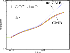
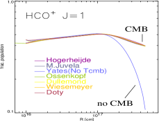
Figure 3: Fractional population of the first two rotational levels of HCO⁺. Panel a) represents the results obtained with seven different codes, while panels b) and c) represent the results obtained with our code by including (b) and excluding (c) the CMBR.

We see that the results agree. Although it cannot be seen in our plots, most of the HCO⁺ in the inner parts of the cloud is in the lowest four rotational levels, because the kinetic temperature is relatively high ($T<20$ K) and there is energy in the medium to populate the higher levels. On the other hand, in the external zones of the cloud, almost 60$\%$ of the HCO⁺ is at the ground level ($J=0$), and the remaining 40$\%$ is in the $J=1$ level due to the lower kinetic temperature, which is not able to populate the higher levels efficiently. As can be seen in Fig. (3a), there is one curve which is different from the others. This is caused by not having included the CMB radiation as the outer boundary condition and assuming that the cloud is not externally illuminated. This turns out to be an extra test for our code, and the results for this particular situation are shown in Fig. (3c). Agreement is also obtained for the remaining levels, and one can see that there is no significant difference between the results in the inner parts of the cloud. However, a totally different result is obtained in the external zones, where the ground level is the only one populated with $\sim$90% of the total abundance. Although the kinetic temperature at the outer envelopes of the cloud is still able to populate higher levels, non-LTE effects produce this underpopulation of the higher levels. Excitation temperature is also plotted in Fig. (4), for the two transitions $J=1\rightarrow 0$ and the $J=2\rightarrow 1$. Also in Figs. (4b) and (4c) the results obtained with our code are also plotted, either including the CMBR as a boundary condition or not, respectively. The results are also comparable to those obtained by different codes in both cases. There is a little more dispersion in this result than in that for fractional population, but this could be due to the fact that the majority of the codes are based on Monte Carlo schemes, which, although they have variance reduction techniques, have an intrinsic random noise that could produce these effects.

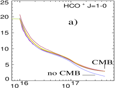
Figure 4: Excitation temperature for the rotational transitions between the three lowest levels of HCO⁺. Panel a) represents the results obtained with seven different codes, while panels (b) and (c) represent the results obtained with our code, either including the CMBR (b) or not (c).

Figure 5: Departure coefficients (right axis) and CO abundance (left axis) in a non-LTE calculation for the $\Delta v=1$ band at 4.7 $\mu$m in a quiet-Sun model. The first five vibrational levels ($v=0$ to $v=4$) with 21 rotational levels ($J=0$ to $J=20$) within each one are included. Note that LTE is obtained for CO in the line-formation region.

3.3 CO in the Sun

We have solved the non-LTE problem for the $\Delta v=1$ ro–vibrational band of CO at 4.7 $\mu$m. The vibrational constant for CO is $\omega_{0}=2143$ cm^-1 and the rotational constant for the vibrational ground state is $B_{0}=1.923$ cm^-1. Since $\omega_{0}\gg B_{v}$, it follows that successive rotational levels within one vibrational state are much closer in energy than similar rotational levels in successive vibrational states. It can be shown that spontaneous radiative decay rates for pure rotational transitions are much lower than collisional rates (see, for example, [Thompson1973]), so one may assume without many problems that the populations of the rotational levels within a vibrational state are given by Boltzmann statistics. This assumption greatly simplifies the problem as shown by [*]uit00 for the same CO problem, because the number of unknowns is reduced from the total number of levels (the number of vibrational levels $\times$ number of rotational levels within each vibrational state) to the total number of vibrational levels. However, we have solved the whole problem without making this assumption and including the first five vibrational levels (from $v=0$ to $v=4$) and 21 rotational levels within each vibrational one (from $J=0$ to $J=20$). A quiet-Sun model atmosphere has been chosen ([Vernazza et al.1981]) and the molecular abundance has been calculated in this model assuming chemical equilibrium. As shown in Fig. (5), the CO abundance peaks at $\sim 300$ km above the bottom of the photosphere. This figure also shows the departure coefficients for all the vibrational levels included. These departure coefficients are calculated as usual, but taking into account the total population of each vibrational level, which can be obtained by summing over the rotational levels inside each vibrational one: $b=\sum_{J}{n_{\rm NLTE}(v,J)}/\sum_{J}{n_{\rm LTE}(v,J)}$. We see that LTE is obtained in the line-formation region below $\sim 800$ km, which is the zone where most of the CO is formed. This partially confirms the results that can be obtained by comparison of the radiative and collisional transition rates.

4 Conclusions

We have generalized very efficient iterative methods for the solution of the molecular radiative transfer problem to spherical geometry with velocity fields. The problem is still one-dimensional, but more angular information is required in comparison to the plane–parallel case, so the total computation time is larger. Velocity fields are treated in the observer’s frame, so velocity fields have to be limited to several times the thermal velocity in the medium if we want to have a tractable frequency quadrature. This limitation is only a computational problem and not a true limitation of the method. Such a fast solution of the non-LTE problem allows the solution of more complicated situations, where larger molecular models can be used. It is known that there can be many different pumping processes in molecular radiative transfer—very important for the interpretation of masers—and a correct model including all the possible important levels is crucial for the interpretation of observations. On the other hand, the advantage of getting the solution of the non-LTE problem in only a few iterations leads to great advantages. This makes it possible to improve the adjusting of all the physical parameters in the model one is using to interpret the observations, because much more extensive forward modeling is now possible. Finally, the fast solution of the radiative transfer problem allows us to introduce the transfer of polarized radiation with the aid of the density matrix theory (see the review by [Trujillo Bueno2001]). This could lead to the self-consistent solution of the maser polarization problem, which could make it possible to explain radio observations of masers such as SiO.

References

- [\astronciteBernes1979] Bernes, C., 1979, A&A, 73, 67
- [\astronciteHogerheijde & van der Tak2000] Hogerheijde, M. R., van der Tak, F. F. S., 2000, A&A, 362, 697
- [\astronciteKunasz & Auer1988] Kunasz, P., & Auer, L. H., 1988, J.Quant. Spectrosc. Radiat. Transfer, 39, 67
- [\astronciteShu1977] Shu, F. H., 1977, ApJ, 214, 488
- [\astronciteThompson1973] Thompson, R. I., 1973, ApJ, 181, 1039
- [\astronciteTrujillo Bueno2001] Trujillo Bueno, J., 2001, in Advanced Solar Polarimetry, M. Sigwarth (ed.) ASP Conf. Series, in press
- [\astronciteTrujillo Bueno & Fabiani Bendicho1995] Trujillo Bueno, J. & Fabiani Bendicho, P., 1995, ApJ, 455, 646
- [\astronciteUitenbroek2000] Uitenbroek, H. 2000, ApJ, 536, 481
- [\astronciteVernazza et al.1981] Vernazza, J.E., Avrett, E.H. & Loeser, R., 1981, ApJS, 45, 635