Radiative Transfer for the $\bf{\cal{FIRST}}$ ERA

Abstract

This paper presents a brief overview of some recent advances in numerical radiative transfer, which may help the molecular astrophysics community to achieve new breakthroughs in the interpretation of spectro-(polarimetric) observations.

1 Introduction

The development of novel Radiative Transfer (RT) methods often leads to important breakthroughs in astrophysical plasma spectroscopy because they allow the investigation of problems that could not be properly tackled using the methods previously available. This RT topic is also of great interest for the “Promise of FIRST”, since a rigorous interpretation of the observations will require to carry out detailed confrontations with the results from NLTE RT simulations in one-, two-, and three-dimensional geometries.

The efficient solution of NLTE multilevel RT problems requires the combination of a highly convergent iterative scheme with a very fast formal solver of the RT equation. This applies to the case of unpolarized radiation in atomic lines, to the promising topic of the generation and transfer of polarized radiation in magnetized plasmas and to RT in molecular lines.

The “dream” of numerical RT is to develop iterative methods where everything goes as simply as with the well-known $\Lambda$-iteration scheme, but for which the convergence rate is extremely high. In this contribution we present an overview of some iterative methods and formal solvers we have developed for RT applications. Our RT methods are based on Gauss-Seidel iteration and on the non-linear multigrid method. These new RT developments are of interest because they allow the solution of a given RT problem with an order-of-magnitude of improvement in the total computational work with respect to the popular ALI method (on which most present NLTE codes are based on). Our RT methods have been succesfully applied to astrophysical problems of unpolarized radiation in atomic lines (in 1D, 2D and 3D with multilevel atoms) and also to the transfer of polarized radiation in magnetized plasmas including anisotropic pumping (Trujillo Bueno, 1999; 2001), which may be of interest for modelling polarization phenomena in MASERS. The case of RT in molecular lines is presented in an extra contribution at this conference by Asensio Ramos, Trujillo Bueno and Cernicharo (2001).

2 RT methods based on Gauss-Seidel iteration

The essential ideas behind the iterative schemes on which our NLTE multilevel transfer codes are based on can be easily understood by considering the “simplest” NLTE problem: the coherent scattering case with a source function given by

$${\rm S=(1-\epsilon)J\,+\,{\epsilon}\,B},$$ (1)

with $\epsilon$ the NLTE parameter, J the mean intensity and B the Planck function. The mean intensity at point “$i$” is the angular average of incoming (“$in$”) and outgoing (“$out$”) contributions. For instance, for a one-point angular quadrature

$${\rm J_{i}}={\rm J_{i}}^{in}+{\rm J_{i}}^{out}{\approx}{1\over{2}}({\rm I}_{i}^{in}+{\rm I}_{i}^{out}).$$ (2)

The well-known $\Lambda-$iteration scheme is to do the following in order to obtain the “${\rm new}$” estimate of the source function at each spatial grid-point “$i$”:

$${\rm S_{i}^{{\rm new}}=(1-\epsilon)J_{i}^{{\rm old}}\,+\,\epsilon\,B_{i}},$$ (3)

where $\rm J_{i}^{{\rm old}}$ is the mean intensity at the grid-point “$i$” calculated using the previous known values of the source function (i.e. using $\rm S_{i}^{{\rm old}}$).

For a given spatial grid of NP points the formal solution of the transfer equation can be symbolically represented as

$${\bf I}_{\Omega}={\vec{\Lambda}}_{\Omega}\,[{\bf S}]\,+\,{\bf T}_{\Omega},$$ (4)

where ${\bf T}_{\bf\Omega}$ gives the transmitted specific intensity due to the incident radiation at the boundary and ${\vec{\Lambda}}_{\bf\Omega}$ is a NP$\times$NP operator whose elements depend on the optical distances between the grid-points. Thus, the mean intensity at the grid-point ”$i$” would be:

$${\rm J_{i}=\Lambda_{i,1}S_{1}^{a}+...+\Lambda_{i,i-1}S_{i-1}^{a}+\Lambda_{i,i}S_{i}^{b}+}$$ (5)

${\rm+\Lambda_{i,i+1}S_{i+1}^{c}+...+\Lambda_{i,NP}S_{NP}^{c}+T_{i}}$.

In this last expression ${\Lambda}_{ij}=\sum({\Lambda}_{ij}^{in}+{\Lambda}_{ij}^{out})/2$ (with the sum applied to all the directions of the numerical angular quadrature) and $a$, $b$ and $c$ are simply symbols that we use as a notational trick to indicate below whether we choose the “${\rm old}$” or the “${\rm new}$” values of the source function. Thus, for instance, the $\Lambda$-iteration method consists in calculating $\rm J_{i}$ choosing $a=b=c={\rm old}$, which gives $\rm J_{i}=J_{i}^{{\rm old}}$ as indicated in Eq. (3).

The Jacobi method, known in the RT literature as the OAB method (from Olson, Auer and Buchler, 1986), and on which most NLTE codes are based on, is found by choosing $a=c={\rm old}$, but $b={\rm new}$, which yields

$${\rm J_{i}=J_{i}^{{\rm old}}\,+\,{\Lambda}_{ii}\,(S_{i}^{{\rm new}}\,-\,S_{i}^{{\rm old}})=J_{i}^{{\rm old}}\,+\,{\Lambda}_{ii}\,{\delta}S_{i}}$$ (6)

In fact, using this expression instead of $\rm J_{i}^{{\rm old}}$ in Eq. (3) one finds that the resulting Jacobi iterative scheme is

$${\rm S_{i}^{{\rm new}}=S_{i}^{{\rm old}}+\delta{S}_{i}},$$ (7)

with the correction

$${\rm\delta{S}_{i}={{[(1-\epsilon)J_{i}^{{\rm old}}+{\epsilon}B_{i}-S_{i}^{{\rm old}}]}\over{[1-(1-\epsilon)\Lambda_{ii}]}}},$$ (8)

where $\Lambda_{ii}$ is the diagonal element of the $\Lambda$-operator associated to the spatial grid-point “$i$”. Note that the correction corresponding to the slowly convergent $\Lambda$-iteration method is given by Eq. (8), but with ${\Lambda}_{ii}=0$.

A superior type of iterative schemes are the Gauss-Seidel (GS) based methods of Trujillo Bueno and Fabiani Bendicho (1995), which can also be suitably generalized to the polarization transfer case (cf. Trujillo Bueno & Landi Degl’Innocenti, 1996; Trujillo Bueno and Manso Sainz, 1999). This type of iterative schemes are obtained by choosing $c={\rm old}$ and $a=b={\rm new}$. This yields

$${\rm J}_{i}={\rm J}_{i}^{{\rm old}\,{\rm and}\,{\rm new}}\,+\,{\Lambda}_{ii}\,\delta{\rm S}_{i},$$ (9)

where ${\rm J}_{i}^{{\rm old}\,{\rm and}\,{\rm new}}$ is the mean intensity calculated using the “${\rm new}$” values of the source function at grid-points 1,2,…,$i-1$ and the “${\rm old}$” values at points $i,i+1,i+2$, …., NP. The iterative correction is given by

$${\rm\delta{S}_{i}^{GS}={{[(1-\epsilon)J_{i}^{{\rm old}\,{\rm and}\,{\rm new}}+{\epsilon}B_{i}-S_{i}^{{\rm old}}]}\over{[1-(1-\epsilon)\Lambda_{ii}]}}}$$ (10)

It is important to clarify the meaning of this last equation:

1) First, at point $i=1$ (which we can freely be assigned to any of the two boundaries of the medium under consideration) use “old” source function values to calculate ${\rm J}_{1}$ via a formal solution. Apply Eqs. (10) and (7) to calculate ${\rm S}_{1}^{{\rm new}}$.

2) Go to the next point $i=2$ and use ${\rm S}_{1}^{{\rm new}}$ and the “old” source-function values ${\rm S}_{j}^{{\rm old}}$ at points $j=2,3,...,$NP to get ${\rm J}_{2}$ via a formal solution. Apply Eqs. (10) and (7) to calculate ${\rm S}_{2}^{{\rm new}}$.

3) Go to the next spatial point $k$ and use the previously obtained “new” source function values at $j=1,2,...,k-1$, but the still “old” ones at $j=k,k+1,...,$NP to get ${\rm J}_{k}$ via a formal solution and ${\rm S}_{k}^{{\rm new}}$ as dictated by Eqs. (10) and (7).

4) Go to the next point $k+1$ and repeat what has just been indicated in the previous point until arriving to the other “boundary point”. Having reached this stage iniciate again the same process, but choosing now as “first point $i=1$” the above-mentioned “boundary point”.

The result of what we have just indicated is a pure GS iteration. Actually, after an incoming and outgoing pass we get two GS iterations! A SOR iteration is obtained by doing the corrections as follows:

$${\rm\delta{S}_{i}^{SOR}}={\omega}\,{\rm\delta{S}_{i}^{GS}},$$ (11)

where $\omega$ is a parameter with an optimal value between 1 and 2 that can be found easily (see Trujillo Bueno and Fabiani Bendicho, 1995).

Figure 1 shows an example of the convergence rate of all these iterative methods applied to a NLTE polarization transfer problem in a stellar model atmosphere permeated by a constant magnetic field that produces a Zeeman splitting of 3 Doppler widths. We point out that the computing time per iteration is similar for all these methods and that matrix inversions are not performed. Thus, the important point to keep in mind is that our implementation of the GS method is 4 times faster than Jacobi (i.e. than the ALI method on which most NLTE codes are based on), while our SOR method for radiative transfer applications is 10 times faster.

Figure 1: The variation of the maximum relative change versus the iteration number for several types of iterative methods applied to the NLTE Zeeman line transfer problem discussed by Trujillo Bueno and Landi Degl’Innocenti (1996). The NLTE parameter $\epsilon=10^{-4}$. Dotted line: the $\Lambda$-iteration method. Dashed line: the Jacobi-based ALI method. Solid line: the GS-based method. Dashed-dotted line: the SOR method.

For pedagogical reasons we have chosen here a NLTE linear problem in order to explain in simple terms our GS-based iterative schemes. The generalization to the full non-linear multilevel problem can be carried out as indicated in the Appendix of the paper by Trujillo Bueno (1999). The critical point is always to remember that the approximations one introduces for achieving the required linearity of the statistical equilibrium equations at each iterative step should treat adequately the coupling between transitions and the non-locality of the problem (see Socas-Navarro & Trujillo Bueno, 1997).

3 The non-linear multigrid RT method

Our GS and SOR radiative transfer methods are based, like the Jacobi-like ALI method, on the idea of operator splitting. Therefore, all of them are characterized by a convergent rate which decreases as the resolution of the spatial grid is increased. As a result, if NP is the number of grid-points in a computational box of fixed dimensions, the computing time or computational work (${\cal W}$) required by the three previous iterative methods to yield the self-consistent atomic (or molecular) level populations scales with NP as follows (cf. Trujillo Bueno & Fabiani Bendicho, 1995):

• Jacobi-based ALI method $\rightarrow\,$ ${\cal W}{\sim}{\rm NP}^{2}$

• Our GS-based RT method $\rightarrow\,$ ${\cal W}{\sim}{\rm NP}^{2}/4$

• Our SOR RT method $\rightarrow\,$ ${\cal W}{\sim}{\rm NP}\sqrt{{\rm NP}}$

Is there any suitable RT multilevel method characterized by ${\cal W}{\sim}{\rm NP}$? This would be of great interest for 3D RT with multilevel atoms where NP$\sim 10^{6}$. The answer is affirmative. This has been worked out by Fabiani Bendicho, Trujillo Bueno and Auer (1997) who considered the application of the non-linear multigrid method (see Hackbush, 1985) to multilevel RT.

The iterative scheme of the non-linear multigrid method is composed of two parts: a smoothing one where a small number of GS-based iterations on the desired finest grid are used to get rid of the high-frequency spatial components of the error in the current estimate, and a correction obtained from the solution of an error equation in a coarser grid. With our non-linear multigrid code the total computational work scales simply as NP, although it must be said that the computing time per iteration is about 4 times larger than that required by the $\Lambda-$iteration method.

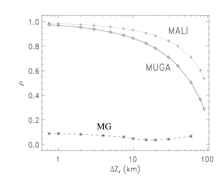
Figure 2: Variation with the grid-spacing $\Delta{z}$ of the maximum eigenvalue of the iteration operator corresponding to several multilevel iterative schemes. The MG symbol refers to our non-linear multigrid code, while MUGA to our multilevel GS-based code. MALI refers to the Jacobi-based multilevel ALI method of Rybicki & Hummer, (1991).

In order to compare the convergence rate of all these iterative methods we present in Fig. 2 an estimate of the maximum eigenvalues ($\rho$) of the corresponding iteration operator, which controls the convergence properties of such iterative schemes. The knowledge of this maximum eigenvalue ($\rho$) is useful because errors decrease as ${\rho}^{itr}$, where “$itr$” is the iterative step. As it can be noted in Fig. 2 the convergence rate of both, the MALI and MUGA schemes decreases when the spatial resolution of the grid is improved, while the maximum eigenvalue of our non-linear multigrid method is always very small ($\rho\sim 0.1$) and insensitive to the grid-size. A maximum eigenvalue $\rho=0.1$ means that the error decreases by one order of magnitude each time we perform an iteration! This explains that, typically, two multigrid iterations are sufficient to reach the self-consistent solution for the atomic level populations.

4 Formal solvers for RT applications

The formal solution routines of our NLTE codes (for unpolarized or polarized radiation and for atomic or molecular species) are based on improvements and generalizations of the short-characteristics (SC) technique introduced by Kunasz & Auer (1988). Let us recall it briefly indicating also our generalization to 3D radiative transfer and to the case of polarized radiation.

The scalar RT equation for the specific intensity is

$${{{\rm d}{\rm I}_{\nu}}\over{{\rm d}{s}}}\,=\,{\chi_{\nu}}\,(\,{\rm S}_{\nu}\,-\,{\rm I}_{\nu}\,)\,,$$ (12)

where $s$ is the geometric distance along the ray propagating in a certain direction in a 3D medium, $\chi_{\nu}$ is the total opacity and ${\rm S}_{\nu}$ the source function.

Point O is the grid-point of interest at which one wishes to calculate the specific intensity ${\rm I}_{\rm O}$, for a given frequency ($\nu$) and a direction (${\vec{\Omega}}$). Point M is the the intersection point with the grid-plane that one finds when moving along $-\vec{\Omega}$. At this upwind point the specific intensity ${\rm I}_{\rm M}$ (for the same frequency and angle) is known from previous steps. In a similar way, point P is the intersection point with the grid-plane that one encounters when moving along $\vec{\Omega}$. We also introduce the optical depths along the ray between points M and O ($\Delta{\tau}_{\rm M}$) and between points O and P ($\Delta{\tau}_{\rm P}$). From the formal solution of the previous transfer equation one finds that

$${\rm I}_{\rm O}={\rm I}_{\rm M}\,{\rm e}^{-\,\Delta{\tau}_{\rm M}}\,+\,\int_{0}^{\Delta{\tau}_{\rm M}}\,{\rm S}(t){\rm e}^{-({\Delta{\tau}_{\rm M}}\,-\,t)}\,dt,$$ (13)

with the optical depth variable measured from M to O.

The integral of this equation can be solved analytically by integrating along the short-characteristics MO assuming that the source function ${\rm S}(t)$ varies parabolically along M,O and P. The result reads:

$${\rm I}_{\rm O}={\rm I}_{\rm M}\,{\rm e}^{-\Delta{\tau}_{\rm M}}\,+\,{\Psi}_{\rm M}{\rm S}_{\rm M}\,+\,{\Psi}_{\rm O}{\rm S}_{\rm O}\,+\,{\Psi}_{\rm P}{\rm S}_{\rm P},$$ (14)

where $\Psi_{\rm X}$ (with X either M, O or P) are given in terms of the quantities $\Delta{\tau}_{\rm M}$ and $\Delta{\tau}_{\rm P}$ that we evaluate numerically by assuming that ${\rm ln}(\chi)$ varies linearly with the geometrical depth, $\chi$ being the opacity.

If the interest lies in the generation and transfer of polarized radiation in magnetized astrophysical plasmas (cf. Trujillo Bueno and Landi Degl’Innocenti, 1996; Trujillo Bueno, 1999; 2001) the situation is a bit more complicated because, instead of having to solve the previous RT equation for the specific intensity, one has to solve, in general, a vectorial transfer equation for the four Stokes parameters. For example, for the standard case of polarization induced by the Zeeman effect, the Stokes-vector at the grid-point O is

$${\bf I}_{\rm O}={\bf O}(0,\Delta{\tau}_{\rm M}){\bf I}_{\rm M}\,+\,\int_{0}^{\Delta{\tau}_{\rm M}}\,{\bf O}(t,\Delta{\tau}_{\rm M})\,{\bf S}(t)\,dt,$$ (15)

where ${\bf O}(t,\Delta{\tau}_{\rm M})$ is the evolution operator (i.e. the 4$\times$4 Mueller matrix of the atmospheric slab between $t$ and $\Delta{\tau}_{\rm M}$). In general, this evolution operator does not have an easy analytical expression and the integral of the previous equation cannot be solved analytically. However, if the 4$\times$4 absorption matrix conmutes between depth points M and O (e.g. because one assumes the absorption matrix to be constant between M and O and equal to its true value at the middle point) the evolution operator reduces then to an expression given by the exponential of the absorption matrix. The integral of Eq. (15) can then be solved analytically provided that the source function vector $\bf S$ is assumed to vary parabolically along M, O and P. Our formal solution method for Zeeman line transfer is precisely based on this idea and the results reads:

$${\bf I}_{\rm O}={\bf O}(0,\Delta{\tau}_{\rm M}){\bf I}_{\rm M}\,+\,{\bf\Psi}_{\rm M}{\bf S}_{\rm M}\,+\,{\bf\Psi}_{\rm O}{\bf S}_{\rm O}\,+\,{\bf\Psi}_{\rm P}{\bf S}_{\rm P},$$ (16)

where $\bf\Psi_{\rm X}$ (with X either M, O or P) are 4$\times$4 matrices which are given in terms of $\Delta{\tau}_{\rm M}$ and $\Delta{\tau}_{\rm P}$, in terms of the inverse of the absorption matrix and in terms of the analytical expression given by Landi Degl’Innocenti and Landi Degl’Innocenti (1985) for the evolution operator for the case in which the absorption matrix is assumed to be constant between the spatial grid points. An alternative formal solver of the Stokes-vector transfer equation suitable for NLTE applications is the one given by Eqs. (1-4) of Socas-Navarro, Trujillo Bueno & Ruiz Cobo (2000).

The application of these formal solution methods in 1D is straightforward. The generalization to 2D geometries with horizontal periodic boundary conditions is substantially more complicated. A suitable strategy has been described by Auer, Fabiani Bendicho and Trujillo Bueno (1994).

The main changes when going to 3D imposing horizontal periodic boundary conditions lie in the interpolation. We have assumed that $\rm I_{M}$ is known but, in most cases, the M-point (like the point P) will not be a grid-point of the chosen 3D spatial grid. The intensity at this M-point has to be calculated by interpolating from the available information at the nine surrounding grid-points, as we must also do for obtaining the opacities and source functions at M and P. Parabolic interpolation can however generate spurious negative intensities if the spatial variation of the physical quantities is not well resolved by the spatial grid. This happens, for instance, if one tries to simulate the propagation of a beam in vacuum using a three dimensional grid. To avoid these problems we have improved the 1D monotonic interpolation strategy of Auer and Paletou (1994), and generalized it to the two-dimensional parabolic interpolation that is required for 3D RT calculations with multilevel atomic models (see Fabiani Bendicho & Trujillo Bueno, 1999).

5 Conclusions

The RT methods presented here are especially attractive because of their direct applicability to a variety of complicated RT problems of astrophysical interest. We emphasize that their convergence rate are extremely high, that they do not require the construction and the inversion of any large matrix and that the computing time per iteration is very small.

References

- [\astronciteAuer, L., Fabiani Bendicho, P., & Trujillo Bueno, J.1994] Auer, L., Fabiani Bendicho, P., & Trujillo Bueno, J., 1994, A&A, 292, 599
- [\astronciteAuer, L., & Paletou, F.,1994] Auer, L., & Paletou, F.., 1994, A&A, 285, 675
- [\astronciteFabiani Bendicho, P., Trujillo Bueno, J.1999] Fabiani Bendicho, P., & Trujillo Bueno, J., 1999, in Solar Polarization, K. N. Nagendra & J. O. Stenflo (eds.), Kluwer Academic Publishers, p. 219-230.
- [\astronciteFabiani Bendicho, P., Trujillo Bueno, J., & Auer, L.1997] Fabiani Bendicho, P., Trujillo Bueno, J., & Auer, L.,1994, A&A, 324, 161
- [\astronciteHackbush, W.1985] Hackbush, W., 1985, Multi-Grid Methods and Applications, Springer Verlag, Berlin
- [\astronciteKunasz & Auer1988] Kunasz, P., & Auer, L. H., 1988, JQRST, 39, 67
- [\astronciteLandi & Landi1995] Landi Degl’Innocenti, E., & Landi Degl’Innocenti, M., 1995, Solar Physics, 97, 239
- [\astronciteOlson, G. L. Auer, L. & Buchler, J. R.1986] Olson, G. L., Auer, L., & Buchler, J. R., 1986, JQRST, 35, 431
- [\astronciteRybicki, G. B. & Hummer, D. G.1991] Rybicki, G. B., & Hummer, D. G., A&A, 245, 171
- [\astronciteSocas Navarro, & Trujillo Bueno2000] Socas Navarro, H., & Trujillo Bueno, J., 1999, ApJ, 516, 436
- [\astronciteTrujillo Bueno1999] Trujillo Bueno, J., 1999, in Solar Polarization, K. N. Nagendra & J. O. Stenflo (eds.), Kluwer Academic Publishers, p. 73-96
- [\astronciteTrujillo Bueno2001] Trujillo Bueno, J., 2001, in Advanced Solar Polarimetry, M. Sigwarth (ed.) ASP Conf. Series, in press
- [\astronciteTrujillo Bueno & Fabiani Bendicho1995] Trujillo Bueno, J., & Fabiani Bendicho, P., 1995, ApJ, 455, 646
- [\astronciteTrujillo Bueno & Landi1996] Trujillo Bueno, J., & Landi Degl’Innocenti, E., 1996, Solar Physics, 164, 135
- [\astronciteTrujillo Bueno & Manso Sainz1999] Trujillo Bueno, J., & Manso Sainz, R., 1999, ApJ, 516, 436