Searching for fluctuations in the IGM temperature using the Lyman $\alpha$ forest

Abstract

We propose a statistical method to search for fluctuations in the temperature of the intergalactic medium (IGM) using the Lyman $\alpha$ forest. The power on small scales ($\sim 25\ {\rm km}/{\rm s}$) is used as a thermometer and fluctuations of this power are constrained. The method is illustrated using Q1422+231. We see no evidence of temperature fluctuations. We show that in a model with two temperatures that occupy comparable fractions of the spectra, the ratio of small scale powers is constrained to be smaller than $3.5$ (corresponding to a factor of $2.5$ in temperature). We show that approximately ten quasars are needed constrain factors of two fluctuations in small scale power power.

1. Introduction

The Lyman $\alpha$ forest has become one of the major tools of cosmology. It has been used to set constraints on many of the parameters of the cosmological model, such as the amplitude and slope of the spectrum of primordial density fluctuations and the nature of the dark matter (Croft et al. (1998, 1999); White & Croft (2000); Narayanan et al. (2000); Zaldarriaga, Hui & Tegmark (2000); Croft et al. (2000)). In the popular cosmologies, the forest arises rather naturally and both cosmological simulation (Cen et al. (1994); Hernquist et al. (1995); Zhang et al. (1995); Miralda-Escude et al. (1996); Muecket et al. (1996); Wadsley & Bond (1996); Theuns et al. (1998)) as well as analytical models have been used to understand its properties (Bi et al. (1992); Reisenegger & Miralda-Escude (1995); Bi & Davidsen (1997); Gneidn & Hui (1996); Croft et al. (1997); Hui & Gnedin 1997a ; Hui et al. 1997b ).

The statistical properties of the forest flux are affected by the physical properties of the intergalactic medium (IGM) such as its temperature or the slope of its equation of state affect. In turn these physical properties of the IGM are sensitive to the ionization history of the universe and the cosmological parameters. An intensive effort has been devoted to understanding what different scenarios predict for the forest and in constraining those scenarios with the available observations (eg. Hui & Gnedin 1997a ; Gnedin & Hui (1998); Schaye et al. (1999); McDonald et al. (2000); Croft et al. (2000)).

The temperature of the IGM has been determined in two different ways, by measuring the widths of the lines (Schaye et al. (1999); McDonald et al. (2000)) and by studying the small scale power spectrum of the flux (Zaldarriaga, Hui & Tegmark (2000)). Both methods find values of the temperature around $T\sim 20,000K$ which are higher than theoretical expectations (ie. Hui & Gnedin 1997a ; Hui et al. 1997b ). Both these type of studies as well as most theoretical models assume that the temperature of the IGM is constant in space. The aim of this paper is to formulate a method for testing this assumption, illustrate it using the spectrum of one quasar and investigate what type of constraints on the temperature fluctuations could be obtained with more data.

A possible explanation for the high temperature of the IGM around redshift $z\sim 3$ is heat deposited in the gas by the double ionization of He. Depending upon the nature of the source responsible for the reionization of the universe and its clumpiness, HeII reionization can be substantially delayed relative to H reionization and could happen around $z\sim 3$ (Miralda-Escude & Rees (1994); Madau & Meiksin (1994); Miralda-Escudé et al. (2000)).

A natural consequence of this scenario are fluctuations in the temperature of the IGM around $z\sim 3$. In fact studies of the HeII Lyman $\alpha$ forest show that the mean absorption is increasing rapidly with redshift for redshifts between 2 and 3. Moreover several gaps of size $\sim 1000{\rm km}/{\rm s}$ where the transmitted flux is high have been observed (Reimers et al. (1997); Anderson et al. (1998); Heap et al. (2000); Smette et al. (2000)).

A uniform IGM temperature has been assumed in most of the theoretical and observational Lyman $\alpha$ forest work so far. We live in an inhomogeneous universe, inhomogeneous heating of the IGM due to a late HeII reionization is only one of the possible sources of temperature fluctuations. It is timely to investigate possible ways of detecting temperature fluctuations. In this paper we use the small scale power spectrum of the forest flux as a measure of temperature (Theuns et al. (2000); Zaldarriaga, Hui & Tegmark (2000)) an introduce the tools necessary to search for fluctuations in the small scale power.

The paper is organized as follows, in section §2 we summarize the properties of the small scale power spectrum and its dependence on the IGM temperature, in §3 we introduce the tools we use in the search for temperature fluctuations, in §4 we apply our technique to Q1422+231 (Kim et al. (1997)), a quasar at redshift $z=3.62$ and in §5 we estimate how much data is needed to substantially improve our constraints. We conclude in §6

2. The power spectrum as a measure of the IGM temperature

The power spectrum of the flux in the Lyman $\alpha$ forest can be used as an indication of the IGM temperature (Theuns et al. (2000); Zaldarriaga, Hui & Tegmark (2000)). Figure 1 shows the predictions of a set of models with different temperatures together with the measurements of McDonald et al. (1999). The simulations used in this paper are described in Zaldarriaga, Hui & Tegmark (2000). We use PM simulations to solve for the dark matter and then use analytic scaling relations to construct mock flux spectra. Our simulations have $128^{3}$ particles in a box that at $z=3$ is $3200{\rm km}/{\rm s}$ in size.

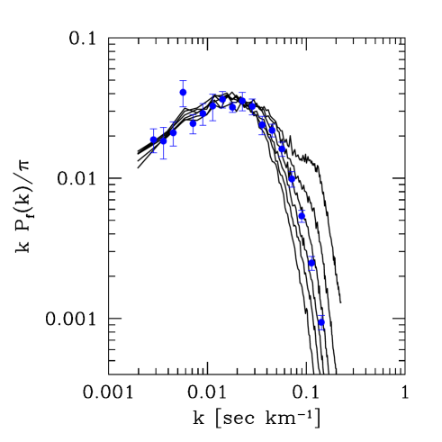
Figure 1.— Transmission power spectrum from Zaldarriaga, Hui & Tegmark (2000). Models with have varying $T_{0}$ ($T_{0}=(150,250,\cdots 650)({\rm km}/{\rm s})^{2}$ increases from top to bottom, $\gamma$ was set to $0.2$ and the mean transmission was set to $0.7$). The data points are from McDonald et al. (1999).

Given that the small scale power is sensitive to the temperature of the IGM it is reasonable to try to detect fluctuations in the IGM temperature by searching for fluctuations in the small scale power. To do so we have to measure the power in different positions along the spectrum and/or on lines of sight towards different quasars. We could use Fourier analysis on pieces of the spectra but we prefer to use wavelets, a natural tool to obtain measures of power that are simultaneously localized in real and frequency space. In the next section we review the properties of the wavelet expansion that are relevant for our work.

3. Wavelets

Wavelets have been used in a number of statistical studies of the forest. In Meiksin (2000) wavelets were introduced for data compression and several statistical properties of the wavelet coefficients were presented.

For our purposes the more relevant work is that of Theuns & Zaroubi (2000). Just as we will do in this paper, the authors used wavelet coefficients to measure the small scale power in the spectrum. They presented the cumulative probability distribution of the squares of the wavelet coefficients and focus most of their effort on comparing models with different temperatures and equations of state and thus different small scale power. They conclude that the wavelet coefficients in these different models have different enough distributions to be able to tell the models apart observationally. In Zaldarriaga, Hui & Tegmark (2000) we used Fourier analysis and measurements of the small scale power in the literature to constrain the equation of state of the IGM. Both Theuns & Zaroubi (2000) and Zaldarriaga, Hui & Tegmark (2000) are very similar in this respect, they propose the same “thermometer” for the IGM, the small scale power in the forest.

Furthermore, Theuns & Zaroubi (2000) argue that because wavelet coefficients are localized in real space they can be used to measure fluctuations in the temperature. They showed results for the cumulative distribution of a model with two temperatures and compare them to models with one single temperature. Unfortunately it is unclear how much of the difference is due to the models having a different mean temperatures and how much is due to the fluctuations themselves, or how much data is needed to get tight constraints on fluctuations. Our work in this paper builds on the ideas presented in Theuns & Zaroubi (2000) and Zaldarriaga, Hui & Tegmark (2000) with special focus on statistical tests of temperature fluctuations.

In this section we introduce the concepts necessary to understand the use of wavelets in the context of this paper.

3.1. Definitions

The best way to introduce the necessary concepts is by looking at the wavelet decomposition of a piece of spectra from Q1422+231 (Kim et al. (1997)). In figure 2 we show $3200\ {\rm km}/{\rm s}$ of the spectra together with wavelet coefficients. This is approximately a 10th of the Lyman $\alpha$ part of the spectra. We will use all the spectra later, here we chose to show a small portion mainly for clarity but also because this is the length of the simulations we will have to compare with. The wavelet transform of the spectra is obtained by convolving the spectra with a set of test functions which we will call $\psi_{n}(x-x_{i})$,

$$a_{n}(x_{i})=\int dxF(x)\psi_{n}(x-x_{i}),$$ (1)

$x$ denotes position along the spectra and $F(x)$ is the flux. The test functions are characterized by two numbers, the index $n$ and $x_{i}$. Increasing values of $n$ correspond to higher spatial frequencies, $x_{i}$ determines the position of the wavelet along the spectrum. The values of $x_{i}$ are determined by the wavelet scheme. For the wavelets we are using there are $2^{n}$ values of $x_{i}$ in each order $n$. Figure 2 shows a few examples of these wavelets to illustrate how as $n$ increases, the wavelet corresponds to higher spatial frequencies. In this work we use the Daubenchies 4 wavelets implemented in a Numerical Recipes routine (Press et al. (1992)).

Figure 2.— Wavelet transform of $3200{\rm km}/{\rm s}$ of the spectrum of Q1422+231. On the top we show the actual spectrum. In the middle panels we plot the amplitude of the wavelet coefficients along the spectra for four different orders. In the bottom panel we show examples of the wavelet functions $\psi$ for the orders whose coefficients are shown.

For our purposes the wavelets are just a set of filters that we apply to the data. They have the advantage of being localized in both Fourier and spatial domain, of being an orthogonal and complete set, and perhaps most importantly that packages that perform the transform are readily available.

To further de-mystify the wavelets we can look at the power spectrum of the forest from a wavelet perspective. Rather than computing squares of Fourier coefficient we can obtain a measure of power by averaging the squares of the wavelets coefficients of a fixed $n$ but different positions along the spectrum. We have

$$\hat{P}\propto{1\over N}\sum_{i=1}^{N}a_{n}^{2}(x_{i}),$$ (2)

the constant of proportionality depends on the normalization convention of $\psi_{n}$. The wavelets are well localized in real space so they must have a broad response in Fourier space. These response or window functions for a few orders are shown in figure 3. By construction window functions of successive $n$ differ only by a factor of 2 scaling in the $x$ axis. In figure 3 we also show the power spectrum measured in the conventional Fourier way or using wavelts. The $x$ coordinate of each wavelet measurement is set to the peak of the window function, but the windows are clearly very broad.

We should point out that the $n$ label is arbitrary in the sense that the label for a wavelet that probes a particular range of spatial scales depends on the length of the spectrum being analyzed. For example, if we start with a piece of spectrum that is twice as long ($6400\ {\rm km}/{\rm s}$) all the labels would be shifted by one. That is, the new $n=7$ wavelet probes the same scales as the old $n=6$ did. As long as one is consistent with the normalization convention the new wavelet coefficients of order $n+1$ will be equal to the old coefficients of order $n$ at the same position along the spectrum. To avoid confusion we will use the labels corresponding to $3200{\rm km}/{\rm s}$ in all our discussions even when we analyze the full length of Q1422+231 spectrum. Figure 3 indicates exactly what scales we probe when we discuss each order $n$.

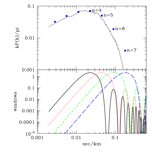
Figure 3.— In the top panel we show the power spectrum of the forest in a cosmological simulation measured both using Fourier and wavelet analysis. The line corresponds to Fourier analysis, the points are the equivalent measures using wavelets. On the bottom we show the window functions for the $n=4,5,6,7$ wavelets. The power measured using wavelets is a weighted average of the Fourier power spectrum with the windows as weights.

It is useful to discuss how the power in the wavelet coefficients depends on the temperature. In figure 4 we illustrate the rate of change of power with temperature obtained in our simulations. Clearly the smallest spatial scales are most sensitive. The figure also shows that for $n=7$ a factor of $2$ change in the temperature, which could be expected in models were He has been doubly ionized in patches of the spectrum, could lead to a factor of $2.5$ change in the observed power. For the figure me assumed an isothermal model, the temperature of the gas is independent of its density. In Zaldarriaga, Hui & Tegmark (2000) we showed that the small scale power is sensitive to the temperature over a range of overdensities $0.9<\rho/\bar{\rho}<1.8$. The ratio of temperatures in figure 4 should be interpreted as the ratio of temperatures on that range of overdensities. This fact can be particularly important in the case of energy injection by He reionization as the process will not only change the temperature of the gas but also its equation of state, so the relevant parameter is by how much the temperature is increased in the range of overdensities that are probed by the small scale power.

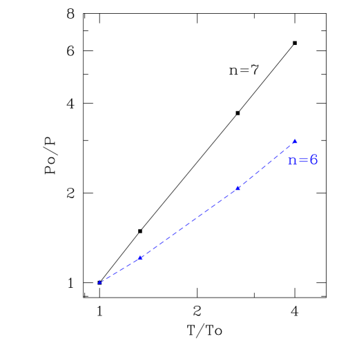
Figure 4.— Ratio of power (average of the square of the wavelet coefficients) for models with different temperatures normalized to a model with $T=300(km/{\rm s})^{2}=1.8\times 10^{4}{\rm K}$ in our simulations. We show the results for $n=6$ and $n=7$ wavelets.

In summary wavelets of different scales $n$ measure power on different spatial frequencies. Their frequency response is broad, the trade-off for the wavelets being localized in real space. The wavelets probing the small scales are very sensitive to the temperature of the IGM and we will use these coefficients as probes of the temperature. We will take advantage of the localization in real space of the wavelets to search for temperature fluctuations.

3.2. Statistical properties of the wavelet coefficients

Now that we have defined the wavelet coefficients we will turn to some analysis of their statistical properties in the case of the Lyman $\alpha$ forest flux.

In the rest of the paper we will be interested in the small scale power, that we will be using as a thermometer. In figure 5 we show a histogram of the amplitude of the $n=7$ coefficient obtained in our simulations. The variance of this distribution proportional to the flux power spectrum (equation 2). In the the top panel we show the histograms for two different temperatures, $T=400\ (800)\ ({\rm km}/{\rm s})^{2}=2.4\ (4.8)\times 10^{4}{\rm K}$. Clearly the model with the largest temperature has the smaller small scale power, the variance of the distribution is smaller.

In the bottom panel of figure 5 we have rescaled the $x$ axis by dividing it by the variance. The two histograms now fall on top of each other, although there are some small differences. For comparison we also show the histograms of the coefficients of Q1422+231 which have a distribution which is remarkably similar to the coefficients in the simulation.

In figure 5 we show a Gaussian together with the histograms of the coefficients in the simulations and in Q1422+231. There are clear differences between the Gaussian and the rest. The amplitudes of the wavelets of the flux have a probability of being near zero which is much larger than one would expect in a Gaussian of the same variance. This is clearly noticeable in the example of figure 2, several stretches of the spectrum can be identified where the amplitude of the wavelet coefficients are very small. The distribution of the coefficient on the simulation also has tails, it is much probable to get large coefficients than in a Gaussian distribution.

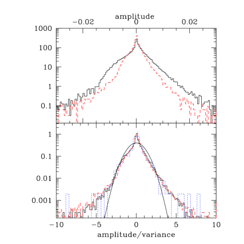
Figure 5.— In the top panel we show the histograms of the amplitude of $n=7$ wavelet coefficients in our $3200{\rm km}/{\rm s}$ simulations for two different temperature, $T=400({\rm km}/{\rm s})^{2}$ (larger variance) and $T=800({\rm km}/{\rm s})^{2}$ (smaller variance). In the bottom panel we have rescaled the axis using the variance. We also show the distribution for the coefficients of $Q1422+231$ (dotted line) and a simple Gaussian (solid line).

To lay the foundation for our method to probe for temperature fluctuations we also need to study the spatial correlations of the wavelet coefficients. In figure 6 we show the correlation coefficient of the wavelet amplitudes ($CC$) as a function of separation along the spectra ($\delta v$) for several scale indices $n$,

$$CC(\delta v)={<a_{n}(x)a_{n}(x+\delta v)>\over<a_{n}^{2}>}.$$ (3)

The correlation coefficient decays fast with separation and then levels off at a value below $1\%$. In our future analysis we will be considering only the smaller scales, corresponding to $n=6$ or $7$. The correlations in these cases become negligible (below $1\%$) for separations larger than $\sim 100{\rm km}/{\rm s}$.

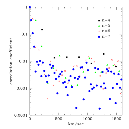
Figure 6.— Correlation coefficient for wavelets of different indices $n$ as a function of separation $\delta v$. For the smallest scales ($n\leq 6$ the correlations become negligible ($<1\%$) foe separations larger that $\sim 100{\rm km}/{\rm s}$.

3.3. Analytic tools

In order to detect temperature fluctuations we want to look for variations in the statistical properties of the wavelet coefficients as we look at different parts of the spectra or as we compare different lines of sight. It is clear that any statements about fluctuations will be statistical in nature, the variance in the distribution of the wavelet coefficients is our thermometer, not the coefficients themselves. Thus we cannot measure the temperature on a pixel by pixel basis, we need to average over many pixels.

Our measure of power is the square of the wavelet coefficient, thus we will introduce averages of the square of these coefficients which we will call $w$,

$$w={1\over N_{p}}\sum_{i}a_{n}^{2}(x_{i}).$$ (4)

The sum is done over contiguous portions of the spectra of length $L$. Different portions do not overlap, and there are $N_{p}$ coefficient in each chuck of size $L$. $N_{p}$ depends on the order $n$ one is considering, $N_{p}=2^{n}(L/3200{\rm km}/{\rm s})$. By definition the mean of $w$ is the measure of power and thus temperature. The mean only depends on the index $n$ and not on $L$. In figure 7 we show the histogram or probability distribution (PDF) of $w$ for several choices of $L$ in our simulation. We show the histograms for two temperatures. It is clear from the figure that the model with the larger temperature has a smaller mean $w$.

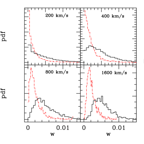
Figure 7.— Probability distribution function of $w$ (defined in equation 4) for four different choices of $L$ and $n=7$. Each panel shows two temperatures,$T=400({\rm km}/{\rm s})^{2}$ (larger mean) and $T=800({\rm km}/{\rm s})^{2}$ (smaller mean). The mean of $w$ is independent of $L$, it depends on the temperature and $n$.

In figure 8 we have rescaled the $x$ axis in figure 7 using the mean of $w$ ($\bar{w}$) for each temperature. The histograms for the two temperatures are quite similar, we are thus encouraged to find some simple analytic model. Our statistic $w$ is an average of squares of many variables which as figure 6 shows quickly become uncorrelated. We could expect that a $\chi^{2}$ distribution would be a good model for the observed distributions. The effective number of degrees of freedom $\nu$ of the $\chi^{2}$ distributions need to be determined. Furthermore because the different panels correspond to values of $L$ that increase by factors of 2, the effective number of degrees of freedom should increase by factors of 2. In figure 8 we plot this simple analytic approximation,

$$P(w|\bar{w}) = {\nu\over\Gamma(\nu/2)2\bar{w}}\ \ e^{-u}\ \ u^{\nu/2-1}$$

$$u = {w\nu/2\bar{w}},$$ (5)

where for the different panels we choose $\nu=1,2,4,8$. Changing slightly the values of $\nu$ improves or worsens the agreements depending on the panel. We choose these values doing a simple $\chi$ by eye of the above plots. Our constraints on the temperature fluctuations are insensitive to the details of this choice, different values of $\nu$ give the same answer, as long as the analytic formulas fit the panels reasonably well. Note also that the distribution for the data of Q1422+231 is also quite similar, there are some differences for the largest smoothing window but in that case there are only a few samples Q1422+231, so the discrepancy is not significant.

We will use this analytic form for the pdf of $w$ throughout the rest of our work. Although the approximation is not perfect our analytic formulas give a good description what is observed in the simulations. We are going to be searching for variations in this distribution as we move along the spectra, so it is very useful that we have an analytic form and furthermore that this analytic form depends on only one parameter $(\bar{w})$. When formulated this way, the question of fluctuations in the temperature can be very simply stated. Does a model with a single value of $\bar{w}$ fit the data better than a model were $\bar{w}$ varies in some particular way across the spectrum.

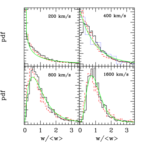
Figure 8.— Rescaled probability distribution function of $w$ for four different choices of $L$ and $n=7$. Each panel shows two temperatures, $T=400({\rm km}/{\rm s})^{2}$ (solid) and $T=800({\rm km}/{\rm s})^{2}$ (dashed) together with our analytic model. In addition in the $L=400{\rm km}/{\rm s}$ panel (the smoothing scale we use in our statistical study) we show the pdf for Q1422+231.

We could take a different approaches to look for fluctuations in the statistical properties of the coefficient. We could directly compare the observed distributions with what is obtained in simulations where a uniform temperature was assumed and search for differences. The problem with this approach is that one must establish that this differences are not a consequence of systematic effects introduced in the simulation process by some missing physics or some numerical artifact. We believe that our method is more robust as it does not use simulations directly, only to motivate our choice of distribution. We are essentially looking for changes in the parameters of the distribution we use to model the data as we go along the spectrum. Any change in this parameters is a signal of fluctuations even if our distribution is not a perfect model of the data.

4. Constraints on temperature fluctuations

Our objective is to use the small scale power as a thermometer, and this thermometer to search for fluctuations. In the previous sections we have established a model for the probability distribution of the square of the wavelets coefficients. This model is dependent on one parameter, which we chose to be the mean power on that scale. The objective of this section is to describe the formalism necessary to constrain spatial fluctuations in the mean power, such as those that would be produced by fluctuation in the temperature.

Let as call ${\bf w}$ the vector with the square of the amplitude of the wavelet coefficient as a function of position along the spectra. Let us denote $N$ the dimension of that vector, which is given by the ratio of the length of the spectrum to length of the averaging filter in equation (4). For simplicity we will call each of the entries of these vectors pixels, although they are a combination of several pixels in the initial spectrum.

In the previous sections we found a model for ${\rm P}(w_{i}|\bar{w}_{i})$, the probability of measuring $w_{i}$ given that mean $\bar{w}_{i}$ of $w$ at position $i$ along the spectrum, (equation 3.3). To describe our model for the fluctuation we need to introduce another vector ($\bar{\bf w}$) that specifies the value of $\bar{w}$ along the spectrum. The dimension of $\bar{\bf w}$ is also N. The probability of measuring the vector ${\bf w}$ is given by,

$${\rm P}({\bf w}) = \int d\bar{\bf w}{\rm P}(\bar{\bf w}){\rm P}({\bf w}|\bar{\bf w})$$ (6)

$$= \int d\bar{w}_{1}\cdots d\bar{w}_{n}{\rm P}(\bar{\bf w})\prod_{i=1}^{N}{\rm P}(w_{i}|\bar{w}_{i}).$$

Different models for the temperature distribution differ in what ${\rm P}(\bar{\bf w})$ is. For example for a uniform temperature model where for every pixel the mean power is $\bar{w}$ we have,

$${\rm P}(\bar{\bf w})=\delta^{D}(\bar{w}_{1}-\bar{w})\cdots\delta^{D}(\bar{w}_{N}-\bar{w})\$$ (7)

By combining equations (3.3), (6) and (7) we obtain the probability of measuring ${\bf w}$ under the assumption that the temperature is uniform (${\rm P}^{u}$),

$$\ln{\rm P}^{u} = \sum_{i}\ln{\rm P}(w_{i}|\bar{w})$$ (8)

$$= \sum_{i}(\nu/2-1)\ln(u_{i})-u_{i}$$

$$- N\ln[2\bar{w}\Gamma(\nu/2)/\nu],$$

where $u_{i}=w_{i}\nu/2\bar{w}$.

We want to constrain fluctuations in the temperature by comparing the probability of having measured a vector ${\bf w}$ in a particular model for the temperature fluctuations (${\rm P}^{f}$) with the same probability in a uniform temperature model (${\rm P}^{u}$). The ratio of ${\rm P}^{f}$ and ${\rm P}^{u}$ is the likelihood ratio for the two models. In order to compute ${\rm P}^{f}$ we need to specify the value of ${\rm P}(\bar{\bf w})$, our model for the temperature fluctuations. Clearly there are many different choices of ${\rm P}(\bar{\bf w})$ which describe different physical scenarios and it would be impossible for us to try every possibility. Instead in this section we have chosen some particular examples and found constraints in those scenarios.

In all our models we will assume that there are only two different temperature values possible and that the mean power for each of these two temperatures $\bar{w}_{A}$ and $\bar{w}_{B}$, differ by a factor $\beta=\bar{w}_{B}/\bar{w}_{A}$. We will also define $f$ as the fraction of the spectrum with mean $\bar{w}_{A}$. The mean power averaged over all pixels becomes,

$$\bar{w}=f\bar{w}_{A}+(1-f)\bar{w}_{B}.$$ (9)

When comparing different models we will keep this mean, $\bar{w}$ fixed to the observed value in the spectrum. We are not interested in comparing models with different mean power but models with or without spatial temperature fluctuations in the power.

There are two probability ratios that define the problem,

$$\ln{{\rm P}(w_{i}|\bar{w}_{A})\over{\rm P}(w_{i}|\bar{w})} = -u_{i}(1-f)(1-\beta)$$

$$+ {\nu\over 2}\ln(f+\beta(1-f))$$

$$\ln{{\rm P}(w_{i}|\bar{w}_{B})\over{\rm P}(w_{i}|\bar{w})} = -u_{i}f{(\beta-1)\over\beta}$$ (10)

$$+ {\nu\over 2}\ln({f+\beta(1-f)\over\beta}),$$

where $u_{i}=w_{i}\nu/2\bar{w}$. The expressions for ${\rm P}^{f}/{\rm P}^{u}$ in the different models for the fluctuations will always be expressed in terms of these two quantities.

4.1. Independent pixels

We first consider a model in which every pixel is independent of the rest and can be in one of two temperatures, corresponding to mean powers $\bar{w}_{A}$ and $\bar{w}_{B}$. The prior on the small scale power becomes,

$${\rm P}(\bar{\bf w})=\prod_{i}[f\delta^{D}(\bar{w}_{i}-\bar{w}_{A})+(1-f)\delta^{D}(\bar{w}_{i}-\bar{w}_{B})].$$ (11)

The likelihood ratio ${\rm P}^{f}/{\rm P}^{u}$ is,

$$\ln[{\rm P}^{f}/{\rm P}^{u}] = \sum_{i}\ln[f{P(w_{i}|\bar{w}_{A})\over P(w_{i}|\bar{w})}$$ (12)

$$+ (1-f){P(w_{i}|\bar{w}_{B})\over P(w_{i}|\bar{w})}].$$

This expression remains constant if we transform $\beta\rightarrow 1/\beta$ and $f\rightarrow(1-f)$.

We use equation (12) and the full spectra of Q1422+231 to put simultaneous constraints on $f$ and $\beta$ which are shown in figure 9. We do not need to consider values of $\beta<1$ because they can be obtained from $\beta>1$ using the symmetry property of the likelihood ratio. We considered models with a likelihood ratio smaller than 0.05 as ruled out. As can be expected the tightest constraints on $\beta$ are obtained when $f\sim 0.5$. With the data we have we can say that $\beta<3.5$ ($f\sim 0.5$).

As could have been guessed the tightest constraints are obtained when both temperatures occupy a significant fraction of the spectrum, $f\sim 0.5$. However it is interesting to note, that the contour is not symmetric around $f=0.5$. Figure 9 shows that it is harder to put constraints when $f$ is near zero than when it is near one. The reason for this is that when $f\sim 0$ and $\beta>1$, most of the spectrum has the larger small scale power $\bar{w}_{B}$ (low temperature) and only a small fraction has the lower power $\bar{w}_{A}$ (high temperature). Even when $\bar{w}$ is high, figure 8 shows that it is more likely that in any given pixel the value of $w$ is low, thus it is hard to detect the small excess of pixels with low $w$s that is produced by the small fraction of the spectrum that has $\bar{w}_{A}$.

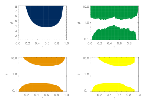
Figure 9.— Two dimensional constraints on the fraction $f$ of spectrum with mean $\bar{w}_{A}$ and ratio $\beta=\bar{w}_{B}/\bar{w}_{A}$. The dark regions have a small likelihood ratio, ${\rm P}^{f}/{\rm P}^{u}<0.05$. The panels correspond to different models for the fluctuation, independent pixels (top left), sharp transition (top right), fixed size bubbles of size $1200{\rm km}/{\rm s}$ (lower left) and of size $2400{\rm km}/{\rm s}$ (lower right).

4.2. Sharp transition

We now consider a case in which there is a sharp transition between $\bar{w}_{A}$ and $\bar{w}_{B}$ which occurs at pixel number $i_{tr}$. The prior becomes,

$${\rm P}(\bar{\bf w})=\prod_{i<i_{tr}}\delta^{D}(\bar{w}_{i}-\bar{w}_{A})\prod_{i>i_{tr}}\delta^{D}(\bar{w}_{i}-\bar{w}_{B}).$$ (13)

The likelihood ratio ${\rm P}^{f}/{\rm P}^{u}$ for this case becomes,

$$\ln[{\rm P}^{f}/{\rm P}^{u}] = \sum_{i<i_{tr}}\ln[{P(w_{i}|\bar{w}_{A})\over P(w_{i}|\bar{w})}]$$ (14)

$$+ \sum_{i>i_{tr}}\ln[{P(w_{i}|\bar{w}_{B})\over P(w_{i}|\bar{w})}].$$

For this model we define $f=i_{tr}/N$. We compute ${\rm P}^{f}/{\rm P}^{u}$ for all possible values of $i_{tr}$ and plot the constraints on $\beta$ in figure 9. We plot the results in terms of $f$ rather than $i_{tr}$. For this model we plot constraints from both $\beta$ bigger and smaller than one, as both cases are not equivalent. One corresponds to a jump from low to high temperature and the other to the opposite case.

These model is the one where the tightest constraints can be obtained because it is the less random. Given $i_{tr}$ the temperature of all pixels is specified. We can can constrain $0.5\leq\beta\leq 2$ for almost all values of $f$.

4.3. Fixed size bubbles

Finally we will consider a case in which there are bubbles of a fixed size with power $\bar{w}_{B}$ and the rest of the spectrum has $\bar{w}_{A}$. To compute the ${\rm P}({\bf w})$ under this scenario we reinterpret equation (6) as an average over ${\rm P}(\bar{\bf w})$ of ${\rm P}({\bf w}|\bar{\bf w})$. We can use a Montecarlo technique to perform this average. We create realizations simply by laying down $N_{b}$ bubbles of a fixed size in the spectrum. We choose randomly the centers of the bubbles. For each realization we compute the likelihood using equation (4) and the average that over all realizations to compute the ${\rm P}({\bf w})$. The model has two free parameters, the size of each individual bubble and the number of bubbles (or equivalently $f$, the fraction of the spectrum having $\bar{w}_{A}$ and $\bar{w}_{B}$).

In figure 9 we show the constraints on $f$ and $\beta$ for two particular bubble sizes, $1200\ {\rm km}/s$ and $2400\ {\rm km}/s$. In this model $\beta$s larger and smaller than one are not equivalent. Our results for independent pixels can be interpreted as a constraint when the typical size of the bubble is $400\ {\rm km}/s$. As can be seen in figure 9 our constraints end up being very similar for all bubble sizes. For $f\sim 0.5$ the ratio of powers have to be in the range $0.3\leq\beta\leq 3.5$.

5. Future

In the previous sections we have developed a method for constraining temperature fluctuations. We illustrated our method using data from Q1422+231. The constraints on the ratio of the powers obtained are somewhat larger than what one might expect to be present in the universe. In this section we compute the number of spectra needed to substantially improve the constraints.

The statistical question we will ask is what constraints on $\beta$ can be obtained from a certain amount of data in the independent pixel model under the assumption that the universe has uniform temperature. Equation (12) implies that the ratio of the probabilities of a uniform model to the fluctuating temperature model (${\rm P}^{f}/{\rm P}^{u}$) is,

$$\ln({\rm P}^{f}/{\rm P}^{u}) = \sum_{i}\ln[f{P(w_{i}|\bar{w}_{A})\over P(w_{i}|\bar{w})}$$ (15)

$$+ (1-f){P(w_{i}|\bar{w}_{B})\over P(w_{i}|\bar{w})}]$$

$$\approx N\int dw{\rm P}(w|\bar{w})$$

$$\ln [f{P(w|\bar{w}_{A})\over P(w|\bar{w})}+(1-f){P(w|\bar{w}_{B})\over P(w|\bar{w})}]$$

In the last line we approximated the sum by a mean over the distribution from which the $w_{i}$ are assumed to be drawn, ${\rm P}(w|\bar{w})$, and we used their independence. The last line of equation (15) is a measure of distance between two probability distribution functions called Kullback-Leibler entropy (Kullback (1959)).

We can set the ratio in equation (15) to $0.05$ and solve for $N$ as a function of $\beta$ and $f$. We show the results in figure 10. We plot only points for $\beta>1$, other values of $\beta$ can be obtained using the transformation $\beta\rightarrow 1/\beta$, $f\rightarrow(1-f)$. We have changed variables form $N$ to $N_{q}$, the number of quasars with the same number of pixels as Q1422+231. The figure shows that ten quasars are needed to obtain constraints on $\beta\sim 2$ for $f\sim 0.5$. The figure also illustrates the fact that it is very difficult to obtain constraints that are much tighter than a factor 2 in $\beta$.

It is interesting to understand why it gets so much harder to obtain constraints when $\beta$ approches one. Figure 10 shows that the number of quasars scales as $N_{q}\propto 1/(\beta-1)^{4}$. The key point is that we are comparing models that by construction have the same mean $\bar{w}$ (the same mean temperature). Thus what we are actually comparing is the variance of the $w$ distribution in both models. We can compute how many samples are needed to distinguish two models that have different variance. We define the variance as $v=<w^{2}>-\bar{w}^{2}$, its value depends on the model (fluctuating or uniform temperature), but $\bar{w}$ is the same across models. We are assuming all the pixels are independant so we can estimate the variance as,

$$\hat{v}={1\over N_{p}}\sum_{i}w_{i}^{2}-\bar{w}^{2}.$$ (16)

The question becomes how many samples $(N_{p})$ are needed to distinguish a model with uniform temperature with one characterized by $\beta$ and $f$. We define the signal to noise ratio as,

$$(S/N)^{2}={[v^{f}-v^{u}]^{2}/{\rm var}(v)},$$ (17)

the ratio of the difference in variance between the model with fluctuations and the one without to the variance of the variance (which we calculate in the uniform model).

In our example the signal to noise ratio becomes,

$$(S/N)^{2}=cN_{p}{(1-\beta)^{4}f^{2}(1-f)^{2}\over[f+\beta(1-f)]^{4}},$$ (18)

where the constant $c$ depends on the shape of the distribution of $w$ and is defined as $c=<w^{2}>^{2}/(<w^{4}>-<w^{2}>^{2})$. The scaling of the signal to noise with the number of pixels is $(1-\beta)^{4}$ as figure 5 shows. It is the fact that we are looking at the difference in the variance of $w$ for models constructed to have the same $\bar{w}$, what makes distinguishing the models so difficult as $\beta\rightarrow 1$. This fact is what forces $N_{q}$ to scale as $1/(\beta-1)^{4}$ instead of $1/(\beta-1)^{2}$.

Finally with more data we could not only get better constraints on model parameters such as $\beta$ but also constrain more ambitious models. For example, rather than have fixed size bubbles we could draw the bubble sizes from some distribution or allow for correlations between their positions. Moreover with more data one has to study in detail certain sources of systematic error in our method like contamination by metal lines or the effect of evolution along the spectra.

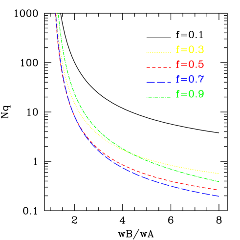
Figure 10.— Number of quasars similar to Q1422+231 needed to obtain a constraint for several values of $f$ as a function of $\beta=\bar{w}_{B}/\bar{w}_{A}$.

6. Conclusions

The uniformity of the temperature in the IGM is an untested assumption in most theoretical modelling of the Lyman $\alpha$ forest. We have presented a statistical method to test this assumption. Our method uses the small scale power of the forest flux as a thermometer and searches for fluctuations in this power. As a result the method is statistical in nature. An important advantage of the method we suggest is that it does not require a direct comparison with numerical simulations. It searches for changes in the statistical properties in different parts of the spectra.

We illustrated our method with Q1422+231. We assumed that in different regions of the spectrum the IGM could be in one of two temperatures. We found that the ratio of small scale power in these two type regions could not differ by more than a factor of $3.5$ if the two type of regions occupy a comparable fraction of the spectrum. This ratio of power translates in a factor of approximately $2.5$ in temperature. If the transition between the two regimes is sharp, the constraints are more stringent, the ratio of powers cannot differ by more than a factor of $2$.

We have calculated how much data is needed to improve this constraints substantially. We showed that ten quasars are needed to constrain fluctuations of factors of two in the power, or equivalently factors of $1.7$ in temperature. Furthermore with more data, more ambitious models for the fluctuations can be considered.

Acknowledgements The author acknowledges very useful comments and suggestions from Joop Schaye and John Bahcall. Support for this work is provided by the Hubble Fellowship HF-01116-01-98A from STScI, operated by AURA, Inc. under NASA contract NAS5-26555.

References

- Anderson et al. (1998) Anderson et al. 1998, preprint astro-ph/9808105
- Bi et al. (1992) Bi H. G., Boerner G., Chu Y.,1992, A&A, 266, 1
- Bi & Davidsen (1997) Bi H. G., Davidsen A. F. 1997, ApJ, 479, 523
- Cen et al. (1994) Cen R., Miralda-Escude J., Ostriker J. P., Rauch M. 1994, ApJ, 437, L9
- Croft et al. (1997) Croft R. A. C., Weinberg D. H., Hernquist L., Katz N. 1997, ApJ, 488, 532
- Croft et al. (1998) Croft R. A. C., Weinberg D. H., Katz N., Hernquist L. 1998, ApJ, 495, 44
- Croft et al. (1999) Croft R. A. C., Weinberg D. H., Pettini M., Hernquist L., Katz N. 1999, ApJ, 520, 1
- Croft et al. (2000) Croft R. A. C., Weinberg D. H., Bolte M., Burles S., Hernquist L., Katz N., Kirman D., Tytler D., astro-ph/0012324
- Gneidn & Hui (1996) Gnedin N. Y., Hui L., 1996, ApJ, 472, 73
- Gnedin & Hui (1998) Gnedin N. Y., Hui L., 1998, MNRAS, 296, 44
- Heap et al. (2000) Heap et al. 2000, ApJ, 534, 69
- Hernquist et al. (1995) Hernquist L., Katz N., Weinberg D. H., Miralda-Escude J. 1995, ApJ, 457, L5
- (13) Hui L., Gnedin N. Y. 1997a, MNRAS, 292, 27
- (14) Hui L., Gnedin N. Y., Zhang Y. 1997b, ApJ, 486, 599
- Kim et al. (1997) Kim T. S., Hu E. M., Cowie L. L., Songaila, A. 1997, AJ, 114, 1
- Kullback (1959) Kullback S., Information Theory and Statistics, Wiley, New York, 1959
- Madau & Meiksin (1994) Madau P., Meiksin A., 1994 ApJ433 L53
- McDonald et al. (1999) McDonald P., Miralda-Escude J., Rauch M., Sargent W. L. W., Barlow T. a. , Cen R., Ostriker J. P., 1999 preprint astro-ph/9911196
- McDonald et al. (2000) McDonald P., Miralda-Escude J., Rauch M., Sargent W. L. W., Barlow T. a. , Cen R., Ostriker J. P., 2000 preprint astro-ph/0005553
- Meiksin (2000) Meiksin A., 2000 preprint astro-ph/0002148
- Miralda-Escude & Rees (1994) Miralda-Escude J., Rees M. 1994, MNRAS, 266, 343
- Miralda-Escude et al. (1996) Miralda-Escude J., Cen R., Ostriker J. P., Rauch M. 1996, ApJ, 471, 582
- Miralda-Escudé et al. (2000) Miralda-Escudé, J., Haehnelt, M. & Rees, M. J. 2000, ApJ, 530, 1
- Muecket et al. (1996) Muecket J. P., Petitjean P., Kates R. E., Riediger R. 1996, A&A, 308, 17
- Narayanan et al. (2000) Narayanan V. K., Spergel D. N., Dave R., Ma C. P. 2000, preprint astro-ph/0001247
- Press et al. (1992) Press W. H., Teukolsky S. A., Vetterling W. T., Flannery B. P., 1992, Numerical Recipes in Fortran (2ed; New York: Cambridge Univ. Press)
- Reimers et al. (1997) Reimers et al. 1997, AA, 327, 890
- Reisenegger & Miralda-Escude (1995) Reisenegger A., Miralda-Escude J. 1995, ApJ, 449, 476
- Schaye et al. (1999) Schaye J., Theuns T., Leonard A., Efstathiou G. 1999, MNRAS, 310, 57
- Smette et al. (2000) Smette A., Heap S. R., Willinger G. M., Tripp T. M., Jenkins E. B., Songaila A., preprint astro-ph/0012193
- Theuns et al. (1998) Theuns T., Leonard A., Efstathiou G., Pearce F. R., Thomas P. A. 1998, MNRAS, 301, 478
- Theuns et al. (2000) Theuns T., Schaye J., Haehnelt M. 2000, MNRAS, 315, 600
- Theuns & Zaroubi (2000) Theuns T., Zaroubi S., preprint astro-ph/0002172
- Wadsley & Bond (1996) Wadsley J. W., Bond J. R. 1996, Proceeding of the 12th Kingston Conference, eds. Clarke D., West M., PASP, astro-ph/9612148
- White & Croft (2000) White M., Croft R. A. C. 2000, preprint astro-ph/0001247
- Zhang et al. (1995) Zhang Y., Anninos P., Norman M. L. 1995, ApJ, 453, L57
- Zaldarriaga, Hui & Tegmark (2000) Zaldarriaga M., Hui L., Tegmark M., astro-ph/0011559