Gas Dynamic Stripping and X-Ray Emission of Cluster Elliptical Galaxies.

Abstract

Detailed 3-D numerical simulations of an elliptical galaxy orbiting in a gas-rich cluster of galaxies indicate that gas dynamic stripping is less efficient than the results from previous, simpler calculations (Takeda et al. 1984; Gaetz et al. 1987) implied. This result is consistent with X-ray data for cluster elliptical galaxies. Hydrodynamic torques and direct accretion of orbital angular momentum can result in the formation of a cold gaseous disk, even in a non-rotating galaxy. The gas lost by cluster galaxies via the process of gas dynamic stripping tends to produce a colder, chemically enriched cluster gas core. A comparison of the models with the available X-ray data of cluster galaxies shows that the X-ray luminosity distribution of cluster galaxies may reflect hydrodynamic stripping, but also that a purely hydrodynamic treatment is inadequate for the cooler interstellar medium near the centre of the galaxy.

1 Introduction

Normal elliptical galaxies contain hot coronal gas which emits radiation in the X-ray band through thermal Bremsstrahlung and collisional line excitation. Total gas masses of the hot interstellar medium (ISM) in elliptical galaxies vary between $10^{8}$ and $10^{10}{\rm M}_{\odot}$, and typical gas temperatures are $T\raisebox{-4.2679pt}{$~{}\stackrel{{\scriptstyle\displaystyle<}}{{\sim}}~{}$}1$ keV, implying that radiative cooling is efficient.

Although, in general, larger elliptical galaxies are also brighter in X-rays, the hot-gas content of elliptical galaxies proves to be very variable, as can be inferred from a scatter plot of the X-ray luminosity $L_{X}$ (in a given waveband) and the blue optical luminosity $L_{B}$ for the observed galaxies (e.g. Irwin & Sarazin 1998). This fact can be related either to the persistence, or otherwise, of a galactic wind sweeping the gas shed from the stellar population of the galaxy (Ciotti et al. 1991), or to the different environments where the galaxies reside. The apparent lack of correlation between the residuals of the $L_{B}$–$L_{X}$ relation and any intrinsic properties of the galaxies in other wavebands may favour the second explanation (White & Sarazin 1991). A gas-rich cluster environment can cause gas dynamic gas-mass loss from (or “stripping” of) the galaxy (Schipper 1974), or also promote radiative cooling by pressure confinement and eventually produce an accretion flow onto the galaxy (Ciotti et al. 1991). The effect of the environment therefore is likely to depend on the size and the depth of the potential well of the galaxy (Bertin & Toniazzo 1995) and on its motion relative to the intra-cluster medium (ICM).

Gas dynamic stripping may be related to the chemical enrichment of the ICM, and possibly also its dynamics (Deiss & Just 1996). A preliminary conclusion from the analysis of X-ray spectra of the ICM is that the metal abundances in the ICM vary from one type of cluster to another, and that the distribution of metals within clusters, especially “cooling flow” clusters, can be non-uniform (Finoguenov, David & Ponman 1999; Irwin & Bregman 2000; De Grandi & Molendi 2000). This suggests that both winds (mainly responsible for [Si] enrichment) and galaxy stripping (resulting mainly in [Fe] enrichment) contribute to the chemical enrichment of the ICM to variable extents, possibly according to the structure of the cluster and the age of the brightest cluster galaxies.

Previous theoretical investigations of gas dynamic stripping (Lea & De Young 1976; Takeda, Nulsen & Fabian 1984; Gaetz, Salpeter & Shaviv 1987; Portnoy, Pistinner & Shaviv 1993; Balsara, Livio, & O’Dea 1994) generally found that ram-pressure stripping of cluster galaxies should be very effective and that a generic cluster elliptical galaxy should retain very little of the gas shed by its stars. Cluster galaxies should thus rarely be very luminous (if detectable) in X-rays. These conclusions are likely to be affected by some assumptions which were made to simplify the mathematical or computational problem. They are not supported by more recent X-ray data, which show that, by contrast, most X-ray bright ellipticals are found within clusters or groups. Careful analysis of high-resolution X-ray data reveals more and more X-ray bright galaxies against the high background of the cluster-gas emission (e.g. Drake et al. 2000). Such evidence indicates that, in general, dense environments host both ISM-depleted and very ISM-rich ellipticals. In the latter, the cooling times of the coronal ISM are short.

Generally speaking, clusters of galaxies at the present epoch appear to be still in the process of accreting smaller groups of galaxies (Dressler & Shectman 1988; Neumann 1997) and single galaxies. In the present work we ask what the hydrodynamic evolution of a galaxy’s ISM will be when an elliptical galaxy is falling into a cluster of galaxies and is moving with respect to the ICM.

To answer this question and update our theoretical understanding of the ISM dynamics of cluster galaxies, a time dependent, three-dimensional, treatment of the hydrodynamic problem, including careful modeling of the “background” galaxy and cluster of galaxies, is desirable.

The generic orbit for a galaxy in a cluster is neither circular nor radial. Instead, it is highly elongated, and describes a rosette-like shape (Binney & Tremaine 1987, §3.1, p.106). As a consequence, the galaxy ‘visits’ regions of the cluster with an ICM at different densities, while its velocity changes both in magnitude and in direction. Furthermore, given a typical temperature of 5-6 keV for the ICM, and a typical velocity dispersion for the cluster of 1000 km/s, it follows that a typical galaxy moves with supersonic speed on a part of its orbit close to the pericentre, and with a subsonic speed near the apocentre. As we show in the next section, this suggests that the dynamics of the ISM-ICM interaction is not two-dimensional, that it is not governed by ram pressure alone, and that it is not steady.

While the central cooling time scale $\tau_{c}$ in an average elliptical galaxy is much longer than the dynamic scale for transonic stripping, optically thin cooling at $T\sim 1$ keV has the tendency of proceeding in a run-away fashion in which $\tau_{c}$ decreases even further unless the gas is completely removed or reheated. When supersonic stripping pauses, the amount and concentration of gas in the galaxy is crucial in determining its further evolution. This fact, together with the greater complexity of a three-dimensional flow, makes simplistic analytical estimates of the efficiency of “ram-pressure” stripping of spiral galaxies (Gunn & Gott 1972; Abadi et al. 1999) unreliable when applied to elliptical galaxies.

Due to the strong feedback of cooling on the dynamics of stripping, one should be careful with allowing for gas “drop out” – gas removal due to radiative cooling – as did Gaetz et al. (1987), Portnoy et al. (1993) and Balsara et al. (1994). Not only does it affect the gas dynamics (Portnoy et al. 1993) but, as we will show, also the long-term evolution of the ISM in the time-dependent problem. On one hand, as long as there are no observational detections of star-formation rates in cluster ellipticals, and there is no compelling theoretical reason for drop out to occur, its inclusion in a time-dependent hydrodynamic calculation is somewhat arbitrary. On the other hand, if stripping was efficient regardless of drop out, neither star formation nor drop out would be needed anymore in the present context.

We perform the first three-dimensional, time-dependent hydrodynamic numerical calculations of this problem. We start from a prescribed initial state (similar to that of Lea & De Young 1976) and include the full radiative cooling due to continuum and line emission. We generally do not allow for drop out, except for comparison with common hydrodynamic models of the X-ray gas (e.g. Sarazin & Ashe 1989). The model we adopt to represent the galaxy (light distribution, gravitational potential) undergoing the stripping process is roughly consistent with well-constrained stellar dynamic models of known cluster elliptical galaxies (Saglia, Bertin & Stiavelli 1992; Dehnen & Gerhard 1994). Mass and energy sources are treated in a standard fluid-average way valid over sufficiently large times and lengths. The cluster ICM and gravitational potential are chosen to be similar to the properties of the Coma cluster. As a result of such detailed modeling, our computations depend on a considerable number of assumptions and parameters, which, however, are not fine tuned but matched as far as possible to current observational knowledge. In order to check the validity of the assumptions and to estimate the reliability of the results in terms of their astronomical implications, we explicitly compare the model results to published X-ray data on bright cluster ellipticals.

The paper is organized as follows. In Section 2 we discuss the time scales of the problem and the main hydrodynamic mechanisms at work in the supersonic flow and in the subsonic flow. In Section 3 we present the relevant equations (Sect. 3.1), the underlying models necessary to calculate the source terms and the gravitational field (Sect. 3.2), and the method of their solution (Sect. 3.3). We discuss also (Sect. 3.3.2) the initial condition and (Sect. 3.3.3) the boundary conditions adopted. In Table 1 the parameters adopted for the four models are summarized. Section 4 contains the main results for the hydrodynamic evolution of the ISM in the four models. In Sections 4.1 and 4.2 we focus on the supersonic and the subsonic part, respectively, in Section 4.3 we discuss the results when drop out is included, and Section 4.4 concerns the long-term evolution determined by the combined effect of the progressive depletion of the outer ISM halo and of the cooling taking place at the galaxy centre. In Section 5 the consequences of stripping on the thermal evolution of the ISM are discussed, with emphasis on the resulting X-ray properties of the halo. In Section 6 we present the computed X-ray morphologies and compare them to X-ray data of well-studied cluster galaxies. In Section 7 we derive some possible implications of the stripping process of cluster galaxies on the ICM. Finally, Section 8 summarizes.

2 Time scales and dimensionality of the hydrodynamic problem

The time evolution of dynamic stripping is governed by five characteristic time scales, which are given by the crossing time $\displaystyle\tau_{cr}=\frac{2L_{gr}}{c_{h}{\rm Ma}}$, the free-fall time $\displaystyle\tau_{ff}=\frac{L_{gr}}{\sqrt{3}\sigma_{*}}$, the cooling time $\displaystyle\tau_{c}=\frac{3nT}{2n_{i}n_{e}\Lambda(T)}$, the Kelvin-Helmholtz (K-H) linear growth time $\displaystyle\tau_{KH}\simeq\frac{3L_{gr}}{c_{h}}$, and the replenishment time $\displaystyle\tau_{rep}=\frac{\rho}{\dot{\rho}_{inj}}$. We have indicated with $L_{gr}$ the gravitational length-scale $L_{gr}\equiv GM/c_{s}^{2}$, where $M$ is the total gravitational mass of the galaxy and $c_{s}$ is the sound speed in the ISM. The quantity ${\rm Ma}$ is the Mach number, $U_{G}/c_{h}$, of the galaxy in the ICM (the more conventional symbol $M$ being used to indicate a mass); $c_{h}$ is the sound speed in the ICM, and typically $c_{s}<c_{h}$; $\dot{\rho}_{inj}$ is the mass-injection rate due to stellar deaths; and $\sigma_{*}$ is the average value of the one-dimensional velocity dispersion of the stars in the galaxy which characterizes the free-fall velocity in the gravitational potential of the galaxy. The factor 3 in the expression for $\tau_{KH}$ is approximate since the K-H growth rate is approximately proportional to ${\rm Ma}$ for ${\rm Ma}>1$ and to $c_{h}/c_{s}$ for ${\rm Ma}<1$ and $c_{h}/c_{s}<1$. Finally, the expression $n_{i}n_{e}\Lambda$ in the cooling time represents the radiated power per unit volume (Eq. (18) in section 3.1). Numerically, these time scales are

$$\displaystyle\tau_{cr}= \displaystyle\frac{2L_{gr}}{c_{h}{\rm Ma}} =47~{}{\rm Myr~{}}\,{\rm Ma}^{-1}\left(\frac{M}{10^{12}{\rm M}_{\odot}}\right)\left(\frac{T_{s}}{\rm keV}\right)^{-1}\left(\frac{T_{h}}{\rm 8keV}\right)^{-1/2}\,,$$ (1)

$$\tau_{KH}= \displaystyle\frac{3L_{gr}}{c_{h}} =70~{}{\rm Myr~{}}\,\left(\frac{M}{10^{12}{\rm M}_{\odot}}\right)\left(\frac{T_{s}}{\rm keV}\right)^{-1}\left(\frac{T_{h}}{\rm 8keV}\right)^{-1/2}\,,$$ (2)

$$\tau_{ff}= \displaystyle\frac{L_{gr}}{\sqrt{3}\sigma_{*}} =49~{}{\rm Myr~{}}\,\left(\frac{M}{10^{12}{\rm M}_{\odot}}\right)\left(\frac{T_{s}}{\rm keV}\right)^{-1}\left(\frac{\sigma_{*}}{\rm 300km/s}\right)^{-1}\,,$$ (3)

$$\tau_{c}= \displaystyle\frac{3}{2}\frac{n}{n_{e}n_{i}}\frac{T}{\Lambda(T)} =540~{}{\rm Myr~{}}\,\left(\frac{T}{\rm keV}\right)^{1.65}\left(\frac{n}{10^{-2}{\rm cm}^{-3}}\right)^{-1}\,,$$ (4)

$$\tau_{rep}= \displaystyle\frac{\rho}{\dot{\rho}_{inj}} =430~{}{\rm Myr~{}}\,\left(\frac{n}{10^{-2}{\rm cm}^{-3}}\right)\left(\frac{\rho_{*}(r_{*})}{10^{-24}{\rm g~{}cm}^{-3}}\right)^{-1}\left(\frac{r}{r_{*}}\right)^{p}\,.$$ (5)

Here, $T_{s}$ and $T_{h}$ are the temperatures of the ISM and the ICM, respectively; $r_{*}$ is a scale radius for the galactic stellar matter distribution, and $p$ is an exponent which varies between $p=4$ for $r>r_{*}$ and $p=2$ for $r<r_{*}$ (Jaffe 1983). Three of the given time scales are ‘fast’, related to the dynamics of pure ablation, pure shear and pure infall, respectively, while the remaining two are ‘slow’, related to local cooling and local mass injection. Because of its dependence on position and on the gas density, mass injection is dynamically relevant near the centre of the galaxy also when stripping is efficient, contributing to the formation of a bow shock in front of the galaxy. In the time-dependent stripping problem, cooling, which is associated with a long time scale, is unimportant only if stripping is complete. In a supersonic flow the gas can be displaced and eventually removed from the galaxy if the condition

$$\rho_{h}c_{h}^{2}{\rm Ma}^{2}\geq\int\rho_{s}\mbox{\boldmath$\nabla$}\Psi_{G}\cdot d{\bf l}$$ (6)

is satisfied (Takeda et al. 1984) for a time of the order of a few crossing times $\tau_{cr}$. In Eq. (6), $\Psi_{G}$ is the galactic gravitational potential, the integral being taken along a path in the direction of the freestream velocity. If the galaxy is not stripped completely, during the time between one pericentre passage and the next, cooling may cause $\rho_{s}$ to increase enough close to the centre (where the gravitational force is strongest) to invalidate Eq. (6). The competition between gas cooling, accretion and gas removal in the subsonic part of the orbit is therefore crucial in determining the evolution of the ISM. The denser ICM near the centre of the cluster causes both ablation of the outer layers and compression of the ISM in the centre, thus favouring central cooling. If cooling proceeds quickly enough, further evolution will be shifted by the very short central cooling time towards net accretion of gas. In general, a given hydrodynamic regime can last only over a time comparable to the time over which the kinetic pressure acting on the ISM does not change significantly, i.e.

$$\displaystyle\tau_{rp} =\displaystyle\left[\frac{d~{}}{dt}\ln(\rho_{C}U_{G}^{2})\right]^{-1}$$ (7)

$$\simeq\displaystyle\frac{rU_{G}}{\sigma_{C}^{2}}\left(2+{\rm Ma}_{r}\right)^{-1}$$

$$\simeq 130~{}{\rm Myr~{}}\,\left(\frac{r_{C}}{500{\rm~{}kpc}}\right)\left(\frac{T_{h}}{8{\rm~{}keV}}\right)^{1/2}\left(\frac{\sigma_{C}}{1200{\rm~{}km/s}}\right)^{-2}\,.$$

This time scale is neither very long compared to the ‘short’ time scales, nor very short compared to the ‘long’ time scales, and implies that the resulting hydrodynamic problem is non-steady and non-linear.

For a general orbit of the galaxy, the time scale $\tau_{rp}$ also determines the rate at which the direction of the free-stream speed varies, modifying the force equilibrium in the ISM. Since $\tau_{rp}$ is shorter than the cooling time, the distribution of the ISM in the galaxy is also affected by the two-dimensional orbital motion of the galaxy. Finally, when the Reynolds number is not small, subsonic stripping depends on the development of Kelvin-Helmholtz modes and on eddy formation, which produce a non-axisymmetric flow even around a galaxy in steady motion along its symmetry axis. The generation of vortices is important in determining the structure of the wake left by the galaxy. A three-dimensional treatment is therefore necessary in order to estimate correctly the drag force on the ISM and the mixing between ISM and ICM.

3 Description of the Model

3.1 Governing Equations

The hot interstellar medium is treated as a Eulerian (non-viscid) ideal monoatomic gas with mass density $\rho$, pressure $p$, temperature $T$ (in energy units) and velocity $u$. The time evolution of these quantities is followed in the reference system of the galaxy which is subject to the acceleration ${\bf g}_{G}$ with respect to the inertial frame of the cluster. The set of equations which determines the time evolution is defined by the hydrodynamic equations:

$$\displaystyle\partial_{t}\rho+\mbox{\boldmath$\nabla$}\cdot\rho\mbox{\boldmath$u$} = \dot{\rho}_{inj}\,,$$ (8)

$$\displaystyle\partial_{t}\mbox{\boldmath$u$}+\left(\mbox{\boldmath$u$}\cdot\mbox{\boldmath$\nabla$}\right)\mbox{\boldmath$u$}+\frac{1}{\rho}\mbox{\boldmath$\nabla$}p = -\mbox{\boldmath$\nabla$}\Psi_{G}+{\bf g}_{G}-\mbox{\boldmath$\nabla$}\Psi_{C}+\frac{\dot{\rho}_{inj}}{\rho}\left(\mbox{\boldmath$u$}_{inj}-\mbox{\boldmath$u$}\right)\,,$$ (9)

$$\displaystyle\partial_{t}\left[\rho\left(\frac{1}{2}u^{2}+\frac{3T}{2\mu}+\Psi_{G}\right)\right]+\mbox{\boldmath$\nabla$}\cdot\left[\rho\mbox{\boldmath$u$}\left(\frac{1}{2}u^{2}+\frac{3T}{2\mu}+\frac{p}{\rho}+\Psi_{G}\right)\right]=\mbox{\hskip 56.9055pt}$$

$$\displaystyle\mbox{\hskip 56.9055pt}\dot{\rho}_{inj}\left(\frac{1}{2}u_{inj}^{2}+\Psi_{G}\right)+\rho\mbox{\boldmath$u$}\cdot({\bf g}_{G}-\mbox{\boldmath$\nabla$}\Psi_{C})+\dot{}\epsilon_{inj}-\dot{}\epsilon_{rad}\,,$$ (10)

complemented by the equation of state

$$p\,=\,nT\,,$$ (11)

and the relations

$$\displaystyle\mu = \rho/n\,,$$ (12)

$$\displaystyle n = n_{i}+n_{e}\,,$$ (13)

$$\displaystyle n_{i} = \frac{\rho}{m_{p}}\sum_{Z}\frac{X_{Z}}{A_{Z}}\;,$$ (14)

$$\displaystyle n_{e} = \frac{\rho}{m_{p}}f_{e}\sum_{Z}\frac{ZX_{Z}}{A_{Z}}\,.$$ (15)

The symbols $\Psi_{G}$ and $\Psi_{C}$ represent the gravitational potential fields generated by the mass distribution of the galaxy and by the mass distribution of the cluster, respectively. We neglect the self-gravity of the gas, so that both $\Psi_{G}$ and $\Psi_{C}$ are given functions of position determined by the assumed galaxy and cluster models. The combination ${\bf g}_{G}-\mbox{\boldmath$\nabla$}\Psi_{C}$ is a tidal field, with the fictitious acceleration ${\bf g}_{G}$ given by

$${\bf g}_{G}=-\mbox{\boldmath$\nabla$}_{{\bf R}_{G}}\Psi_{C}({\bf R}_{G})\,,$$ (16)

where ${\bf R}_{G}=-{\bf x}_{C}$ is the position vector of the galaxy with respect to the centre of the cluster.

The quantities $n$, $\mu$, $n_{i}$, $n_{e}$, $m_{p}$, $f_{e}$, $A_{Z}$ and $X_{Z}$ indicate the total particle number density, the mean mass per particle, the total ion number density, the electron number density, the average mass of one nucleon $m_{p}=1.67\times 10^{-24}$ g, the electron number fraction $n_{e}/n_{i}$, the atomic weight of atoms with atomic number $Z$, and the weight fraction of the atomic species with the atomic number $Z$. The mass of each species is varied only through the distributed mass sources, so that each of the quantities $X_{Z}$ obeys the evolution equation

$$\partial_{t}\left(\rho X_{Z}\right)+\mbox{\boldmath$\nabla$}\cdot\left(\rho X_{Z}\mbox{\boldmath$u$}\right)=\dot{\rho}_{inj}X_{Z,inj}\,.$$ (17)

In the present work only one of the $X_{Z}$’s is varied independently, namely Fe (N=26). The other $X_{Z}$’s are taken to reflect a mixture of “solar” (Anders & Grevesse 1989) and “cosmic” (Wheeler et al. 1989) abundances determined by the ratio [O]/[Fe]. For this reason in our models [Si]/[Fe] = 0.694 [O]/[Fe] + 0.305 in solar units.

The optically thin, collisional radiative cooling term is expressed as usual in terms of a cooling function $\Lambda$:

$$\dot{}\epsilon_{rad}=n_{e}n_{i}\Lambda(T,\underline{X})\,,$$ (18)

where $\underline{X}=\{X_{\rm O},X_{\rm Fe}\}$. We adopt the cooling functions given by Sutherland & Dopita (1993) for conditions of non-equilibrium ionization. For gas cooling at $T<0.1$ keV, ionization equilibrium is not achieved and gas cooling rates are smaller than those derived under that assumption. At higher temperatures, the equilibrium and the non-equilibrium cooling functions are essentially indistinguishable. The cooling coefficient for given $(T,\underline{X})$ is calculated using log-linear interpolation in the temperature $T$, and linear interpolation in the abundance levels. The latter is a fairly good approximation for sub-solar abundances. For $T>$2.7 keV, we extrapolate the cooling function using the pure Bremsstrahlung law $\Lambda\sim T^{1/2}$.

Usually, in steady-state models for the X-ray gas (including the simulation work on steady-state stripping) a sink term $-\dot{\rho}_{do}$ representing gas “drop out” is added on the right-hand side of Eq. (8), with corresponding terms in the energy equation under the assumption that there is no heat exchange between the drop outs and the gas in the flow. Defining the local gas cooling time $\tau_{c}=(3nT/2)/\dot{\epsilon}_{rad}$, we adopt a prescription of the form

$$\dot{\rho}_{do}=q\rho/\tau_{c}\,,$$ (19)

which is found to emulate reasonably well the dynamics of the ISM in X-ray bright galaxies (Sarazin & Ashe 1989; Bertin & Toniazzo 1995). However, we take $q$ to be different from zero for only one model (“Bq”, with $q=0.4$).

Finally, the source terms are given functions of the coordinates:

$$\dot{\rho}_{inj}=\alpha_{*}\rho_{*}(\mbox{\boldmath$x$})\,,$$ (20)

$$\dot{}\epsilon_{inj}=\alpha_{*}\rho_{*}(\mbox{\boldmath$x$})\left[\sigma_{R}^{2}(\mbox{\boldmath$x$})+\sigma_{\phi}^{2}(\mbox{\boldmath$x$})/2+\sigma_{SN}^{2}\right]\,.$$ (21)

Here, $\alpha_{*}$ is the rate of mass return from a passively aging stellar population (Renzini 1988), and it is given by

$$\alpha_{*}=4.75\times 10^{-19}\left(\frac{M_{*}/L_{B}}{{\rm M}_{\odot}/{\rm L}_{\odot}}\right)^{-1}\left(\frac{\tau_{*}}{15{\rm Gyr}}\right)^{-1.3}~{}{\rm s^{-1}}\,,$$ (22)

as a function of the presumed thermonuclear age $\tau_{*}$ of the system, and of the present day (i.e. $\tau_{*}$=15 Gyr, by definition) mass-to-luminosity ratio of the stellar population. We take $\tau_{*}=15$ Gyr initially for all models. The stellar mass density, $\rho_{*}$, and the one-dimensional stellar velocity dispersion components of the stars, $\sigma_{R}$ and $\sigma_{\phi}$, are derived from the models described in the next Section. The additional heating term $\propto\sigma_{SN}^{2}$ is due to Supernovae of type Ia which are supposed to be distributed according to the stellar matter. We assume that each SNIa deposits into the ambient gas an energy of $8\times 10^{50}$ erg. In terms of the rate of SNIa events (events per century per $10^{10}{\rm L}_{\odot}$ blue luminosity), $\displaystyle\sigma_{SN}=1580\,(r_{SN})^{1/2}\,(4.75\times 10^{-19}s^{-1}/\alpha_{*})$ km/s. We take $r_{SN}=0.06$ for $\tau_{*}=15$ Gyr and a Hubble constant $H_{0}=50$km/s/Mpc (Cappellaro et al. 1997). We assume that the ratio of SNIa luminosity to stellar luminosity does not vary in time, so that $\sigma_{SN}$ is constant. Different, and contrasting, assumptions are made in Ciotti et al. (1991) and in Loewenstein & Mathews (1987). The time evolution of the SNIa rate is not known, and our approach is to explore the effects of gas dynamic interactions only and neglect this possible, additional evolutionary effect (see the discussions in Ciotti et al. 1991 and Loewenstein & Mathews 1987).

Finally, both the initial ISM (see Section 3.3.2) and the newly injected gas are assumed to have solar abundances (Anders & Grevesse 1989), with [Fe]/[H]$=2.62\times 10^{-3}$ by weight. The ICM, instead, has “cosmic” abundance ratios (Wheeler et al. 1989) and [Fe]$=0.1~{}$[Fe]_⊙ by weight.

3.2 Input modeling

3.2.1 Galaxy model

The galaxy is represented by the sum of two spheroidal, axisymmetric components, of luminous matter and of dark matter respectively, with densities

$$\rho_{comp}=\frac{(3-\gamma)M_{comp}r_{comp}}{4\pi d_{comp}}m^{-\gamma_{comp}}(m+r_{comp})^{-4+\gamma_{comp}}$$ (23)

where $m^{2}=R^{2}+z^{2}/d_{comp}^{2}$ in cylindrical coordinates, $1-d_{comp}^{2}$ is the eccentricity and the subscript $comp$ denotes either the luminous ($comp=*$) or the dark ($comp=D$) component. We based our treatment on Dehnen & Gerhard (1994), with the inclusion of a second (dark) component, a finite inner core radius (i.e. surface of constant $m$), and a finite cut-off radius. The gravitational potential $\Psi$ and the velocity dispersion profiles $\sigma_{R}$ and $\sigma_{\phi}$ (in the radial and in the azimuthal direction, respectively) are obtained from Eq.(23) using Poisson’s equation and Jeans’ equation, respectively (cf. Binney & Tremaine 1987, §§2.3 and 4.2). We assume that both the stellar and the dark matter have zero bulk rotation.

The values we adopt for the parameters $\gamma_{*}$, $\gamma_{D}$, $r_{*}$, $r_{D}$, $M_{*}/L_{B}$ and $M_{D}/M_{*}$ are taken from the work of Bertin, Saglia & Stiavelli (1992) and Saglia, Bertin & Stiavelli (1992). In these models, the dark halo has a mass and an extension similar or larger than the matter associated with stars (e.g. Saglia et al. 1992; see also Gerhard et al. 1998). We take two parameter sets that reflect the properties of the elliptical galaxies NGC 4472 (M 49) and NGC 4374 (M 84). These two galaxies are bright in X-rays, with typical values of the ratio $L_{X}/L_{B}$ for X-ray bright elliptical galaxies. The parameters for the M49 model are $d_{*}=d_{D}=0.8$, $\gamma_{*}=2$, $\gamma_{D}=1.1$, $r_{*}=16.13$kpc, $r_{D}/r_{*}=2.80$, $M_{*}=7.12\times 10^{11}{\rm M}_{\odot}$ and $M_{D}/M_{*}=1.49$ at a radius of 150kpc. Those of the M84 model are $d_{*}=d_{D}=0.9$, $\gamma_{*}=2$, $\gamma_{D}=1.85$, $r_{*}=16.93$kpc, $r_{D}/r_{*}=1.06$, $M_{*}=3.49\times 10^{11}{\rm M}_{\odot}$ and $M_{D}/M_{*}=1.64$ at a radius of 100kpc. The blue optical luminosities of the two galaxies are $L_{B}=1.1\times 10^{11}{\rm L}_{\odot}$ and $L_{B}=5.8\times 10^{10}{\rm L}_{\odot}$ for NGC 4472 and NGC 4374, respectively. These two models are referred to as ‘GA’ and ‘GB’ in Table 1.

3.2.2 Cluster and Galaxy Orbit

We consider a dynamically relaxed, spherically symmetric, rich cluster of galaxies (like, e.g. the Coma cluster), and we take the ICM distribution to be hydrostatic. The cluster gravitational potential is assumed to be

$$\Psi_{C}(R)=\sigma_{C}^{2}\ln\left[1+\left(\frac{R}{r_{C}}\right)^{2}\right]\,$$ (24)

reflecting a mass distribution close to a non-singular, infinite isothermal sphere with “core radius” for the gravitational mass equal to $2r_{C}/3$. Here, $R$ is the distance from the centre of the cluster, and $\sigma_{C}$ is the one-dimensional velocity dispersion for the self-gravitating mass distribution in the cluster, which gives the velocity scale for the orbital motion of the galaxies. Considering the Coma cluster as a reference, we take $r_{C}=500$ kpc (Briel et al. 1992) and $\sigma_{C}=1201$ km/s (Colless & Dunn 1996).

The temperature profile of the ICM is assumed to be parabolic:

$$T_{C}=\frac{\sigma_{C}^{2}}{\beta_{C}}\left[1-\xi_{C}\left(\frac{R}{r_{C}}\right)^{2}\right]\,,$$ (25)

and, correspondingly, the ICM density profile is

$$\rho_{C}(R)=\rho_{C0}\,\left[1+\left(\frac{R}{r_{C}}\right)^{2}\right]^{-3\bar{\beta}/2}\left[1-\xi_{C}\left(\frac{R}{r_{C}}\right)^{2}\right]^{\bar{\beta}-1}\,,$$ (26)

where $\bar{\beta}\equiv\beta_{C}/(1-\xi_{C})$. For $\xi_{C}=0$ this would be the usual “$\beta$-profile” often taken to fit cluster X-ray halos. However, the ICM in Coma is known not to be isothermal (Arnaud et al. 2000). For this cluster, the central temperature is $\sim 8$ keV while at 800 kpc from the centre the temperature can be as low as 5 keV (Arnaud et al. 2000). Since 8 keV is larger than the ICM temperature of most clusters, we have used two different sets of values for $\beta_{C}$ and $\xi$, one with $\sigma_{C}^{2}/\beta_{C}=6.2$ keV (models A1 and A2) and one with higher central temperature and a steeper gradient (models B and B$q$ –see Table 1).

The model galaxies describe orbits in the potential $\Psi_{C}(R)$. The two orbits considered are shown in the left panels of Fig. 1. They are defined by two quantities, which can be taken as the pericentre $R_{G}^{min}$ and the apocentre $R_{G}^{max}$, and an initial position. We always take the latter to be the apocentre. The two quantities $R_{G}^{max}$ and $R_{G}^{min}$ are given in Table 1 for our models, together with the resulting period of the radial motion.

Note that rich, dynamically relaxed clusters tend to have higher central densities than those given in Table 1. Such dense systems are usually associated to complications such as a central cluster cooling flow, a large cD galaxy with satellites, and nuclear activity. Our models therefore do not apply to the central regions of rich clusters.

3.3 Method of Solution

3.3.1 Numerical scheme

The problem is represented numerically on a three-dimensional, Cartesian grid of points.

The cell size increases from the centre of the galaxy outwards by a factor $p_{m-gr}$ on each successive mesh point. The number of mesh points in each spatial dimension, the central cell size $\Delta_{0}$, and the growth factor $p_{m-gr}$ are listed in Table 1. For models A2 and B two runs were made using different grids, with the aim of comparing the influence of the limited resolution on the results.

The equations are integrated stepwise, alternating conservative hydrodynamic Godunov steps and first-order forward time differencing for sources, cooling, and cluster tidal forces. The hydrodynamic Godunov code (Godunov et al. 1961) used is a version of PROMETHEUS (Fryxell, Müller & Arnett 1989) which implements the Piecewise Parabolic Method (PPM, Colella & Woodward 1984) and Strang splitting (Le Veque 1998). Departures from the equation of state of an ideal gas are accounted for in PROMETHEUS (following Colella & Glaz 1985), although for our computations this is only a small correction. The gravitational acceleration due to the galaxy is treated conservatively (so that the sum of the kinetic energy, the thermal energy and the part of the potential energy arising from $\Psi_{G}$ is conserved by construction), while the cluster tidal forces are included as described in Colella & Woodward (1984). Mass and energy sources, cooling and, when present, drop out have been included consistently in the general time-centred averaging scheme of PPM.

3.3.2 Initial condition

The computation is started at the orbit’s apocentre with an initial gas distribution divided in two different regions. For $r<r_{cut}$, the gas is at constant temperature $T\sim 1$ keV, the metallicity is solar and the velocity (in the grid frame, i.e. the galaxy frame) is zero. For $r>r_{cut}$, the temperature and density are given by the ICM distribution of the cluster model, as explained in section 3.2.2, and the metallicity is 1/10 cosmic. The galaxy is initially in its apocentre and the velocity of the ICM is the opposite of the galaxy’s orbital velocity at the apocentre (the reference system of the calculation is the system of the galaxy). The two regions are connected smoothly via a spherical shell covering the width of 5 cells. The hydrostatic equilibrium condition, i.e. $d(nT)/dr+\rho d\Psi/dr=0$, holds approximately everywhere. We checked that, if the orbital velocity was zero, this initial configuration was stable. The central temperature and density of the ISM are chosen such that there is approximate equilibrium between heating due to energy sources and cooling, and that the central cooling time is comparable to the radial orbital period ($\tau_{c,0}=$ ranges from 1.6 to 2.0 Gyr while $\tau_{orb}$ ranges from 1.6 to 1.9 Gyr in the different models).

These requirements, which result in a central density $n\simeq 10^{-2}$ cm^-3 and a temperature $T\simeq 1$ keV, are motivated by the fact that, on the one hand, we are considering a galaxy that has retained a fraction of order 1/2 of the gas shed by its stars over its lifetime, and that, on the other hand, when a cooling flow sets in, the numerical code loses accuracy and the details of the subsequent evolution become unreliable. While any ‘initial’ state is inevitably arbitrary to some extent, our choice for the initial halo does have the properties of that of a large, gas-rich galaxy which has a central density slightly lower and a central temperature slightly higher than those observed in X-ray bright ellipticals. Under static conditions, as gas accumulated due to continuous injection of matter, the cooling time would become smaller and the heating time longer, thus shifting the balance in favour of cooling-driven accretion. Basically, we ask of our simulations, what evolution results from the competing processes of gas stripping and cooling.

3.3.3 Boundary conditions

The properties of the gas flowing into the grid need to be varied according to the conditions of the ICM around the galaxy. To avoid mismatches at the turning points of the motion along, say, the $x$-axis, the boundary conditions at the (instantaneous) downstream sides should be kept consistent with those on the upstream sides. Thus, we set each quantity at a prescribed value at each boundary point, depending on its position on the grid boundary and on the instantaneous position and velocity of the galaxy in the cluster as calculated from its orbital parameters. We made sure that the grid boundaries are far enough from the galaxy centre (360 kpc for the full runs) so that the gas near the boundaries is not affected by the stripping process, except within the trail of the galaxy. Disturbances artificially generated at the “end” of the trail could not propagate upstream to the galaxy during a half-grid crossing time. Over the remaining part of the grid boundary, velocity mismatches at the boundaries between the gas within the computational grid and that injected into it, caused by the different numerical treatment for the acceleration, were minimal and they did not affect the flow near the galaxy.

The boundary conditions set at the grid bottom are less critical, and we choose to use the same as those set at the grid sides. For the grid top, we compromised between the wish of saving computer time and that of allowing for a true three-dimensional flow without imposing symmetry about the equatorial plane which leads to a suppression of eddy formation. We therefore placed the upper boundary above the symmetry plane of the galaxy by at least half of the galactic half-mass radius, and imposed planar symmetry beyond that boundary, using non-local reflection boundary conditions.

Table 1: Model parameters. Cluster parameters: core radius $r_{C}$, velocity dispersion $\sigma_{C}$, central ICM density $\rho_{C0}$, slope of the $\beta$ model $\beta_{C}$, central ICM temperature $T_{C0}$ and temperature variation parameter $\xi_{C}$. Orbit parameters: apocentre $R_{G}^{max}$, pericentre $R_{G}^{min}$ and orbital period $\tau_{orb}$. Galaxy parameters: model name, scale radius for the galactic stellar matter distribution $r_{*}$, mass of the galactic stellar component $M_{*}$ and blue optical luminosity $L_{B}$. Stellar population parameters: thermonuclear age $\tau_{*}$ and rate of SNIa events per century per $10^{10}{\rm L}_{\odot}$ blue luminosity $r_{SN}$. ISM parameters: central ISM density $\rho_{0}$, central ISM temperature $T_{0}$ and transition radius from ISM to ICM $r_{cut}$. Mass drop out parameter $q$ according to Eq. (19). Grid parameters: number of grid calls in x, y and z direction $N_{x}$, $N_{y}$, and $N_{z}$, respectively, central cell size $\Delta_{0}$, and growth factor $p_{m-gr}$.

	Parameter	A1	$\displaystyle\begin{array}[]{c}{\rm A2}\\ {\rm A2}f\end{array}$	$\displaystyle\begin{array}[]{c}{\rm B}\\ {\rm B}f\end{array}$	Bq
	$r_{C}$ (kpc)	408	408	408	408
	$\sigma_{C}$ (km/s)	1201	1201	1201	1201
	$\rho_{C0}$ ($10^{-27}$ g/cm3)	2.13	2.13	0.165	0.165
Cluster	$\beta_{C}$	1.0	1.0	0.8	0.8
	$T_{C0}$ (keV)	6.2	6.2	7.75	7.75
	$\xi_{C}$	-0.10	-0.10	-0.13	-0.13
	$R_{G}^{max}$ (kpc)	1000	1000	700	700
Orbit	$R_{G}^{min}$ (kpc)	360	360	300	300
	$\tau_{orb}$ (Gyr)	1.9	1.9	1.5	1.5
Galaxy	Model name	‘GA’	‘GB’	‘GA’	‘GA’
	$r_{*}$ (kpc)	16.1	16.9	16.1	16.1
	$M_{*}$ ($10^{11}{\rm M}_{\odot}$)	7.1	3.5	7.1	7.1
	$L_{B}$ ($10^{10}{\rm L}_{\odot}$)	11	5.8	11	11
Stellar	$\tau_{*}$ (Gyr)	15	15	15	15
population	$r_{SN}$ (SNU)	0.06	0.06	0.06	0.06
	$\rho_{0}$ ($10^{-27}$ g/cm3)	14.5	12.5	11.6	11.6
ISM at $t$=0	$T_{0}$ (keV)	1.24	1.24	1.05	1.05
	$r_{cut}$ (kpc)	65	65	105	105
Drop-out	$q$	0.	0.	0.	0.4
	$N_{x}$	82	82	$\displaystyle\begin{array}[]{c}144\\ 100\end{array}$	82
	$N_{y}$	82	82	$\displaystyle\begin{array}[]{c}144\\ 100\end{array}$	82
Grid	$N_{z}$	45	$\displaystyle\begin{array}[]{c}45\\ 71\end{array}$	$\displaystyle\begin{array}[]{c}76\\ 80\end{array}$	45
	$\Delta_{0}$ (kpc)	2	$\displaystyle\begin{array}[]{c}2\\ 0.5\end{array}$	$\displaystyle\begin{array}[]{c}2\\ 0.5\end{array}$	2
	$p_{m-gr}$	1.063	$\displaystyle\begin{array}[]{c}1.063\\ 1.04\end{array}$	1.023	1.063

Figure 1: Left: Galaxy orbital trajectories (thick solid lines, labels indicate elapsed time in Myr) in the cluster ICM distribution (thin solid circles, labels are the decimal logarithm of the ICM density in particles/cm³). Right: kinetic force per unit area of streaming ICM in the reference system of the galaxy (curves labelled by “$\rho U^{2}$”, scale to the left) and upstream Mach number (curves labelled “Ma”, scale on the right). The panels in the upper row apply to models A1 and A2, those in the lower row to models B and B$q$.

3.4 Model Properties

The four models presented are intended to enable us to single out the factors which are most important for the hydrodynamic evolution of the X-ray halo. Relevant model input properties, in principle, are: 1) the total galaxy luminosity and mass; 2) the density of the surrounding gas (ICM) and the velocity (or orbit) of the galaxy; and 3) drop out. Table 1 lists the model parameters adopted for each of the four calculations. Model “A1” and model “A2” differ only in the galaxy model adopted, “GB” being about half as luminous and half as massive as “GA”. Model “A1” and model “B”, instead, have the same galaxy model but different ICM densities and velocities, resulting in an ICM kinetic pressure, $\rho_{ICM}U_{G}^{2}$, 10 times larger for model “A1” than for model “B”. Finally, model “Bq” is identical to model “B”, except that drop out is included, with $q=0.4$. The ICM density of models “A” corresponds to a fairly rich cluster, while the density of model “B” is that of a poor cluster. By comparing the results of the simulations between models, we attempt to derive the general properties of stripping dynamics and to see under which conditions stripping is important.

4 Hydrodynamic evolution

As indicated in Table 1, two different orbits and cluster models were considered. Fig. 1 shows, in the two cases, the orbits of the galaxy against the ICM background density, and the Mach number and the momentum flux of the corresponding flow upstream of the galaxy in the reference frame of the galaxy.

In Fig. 2 the net mass-loss rates, corrected for mass injection and drop out, are given. In the absence of hydrodynamic interaction the galaxy would accumulate the gas shed by its stars, either in gaseous form or in the form of drop outs. This situation is referred to as zero mass loss (or gas accumulation). When gas is lost from the galaxy, the mass-loss rate is defined as

$$\dot{M}_{ISM}=\int{-\dot{\rho}+\dot{\rho}_{inj}-\dot{\rho}_{do}\,d^{3}x}$$ (27)

where $\dot{\rho}$ is the time derivative of the gas density, $\dot{\rho}_{inj}$ and $\dot{\rho}_{do}$ are the mass injection and the mass drop-out terms as defined in Eqs.(19) and (20), and the domain of integration extends over a suitably defined portion of space associated to the galaxy. Unless stated otherwise, we will usually refer to the volume enclosed within a distance $r_{*}$ from the galaxy centre. Except for the first large stripping event, this estimate turns out to be very close to that obtained when summing over all computational cells in which the gas has a negative total energy density in the galaxy’s reference frame, i.e. $\rho u^{2}/2+\rho\Psi_{G}+3nT/2<0$.

The panels corresponding to models A1 and B show that the hydrodynamic evolution entails not only gas loss, but also more or less prolonged phases of gas accumulation or even accretion (negative mass loss).

Figure 2: Net ISM mass-loss rate as a function of time for the four models presented, as labelled in the upper-right corner of each panel. The dots represent the ratios of the increments in gas mass to the increments in time, for the gas contained within a radius $r_{*}$ of the galaxy. The time resolution of the simulation data output rate was typically 15-20 Myr, or 100 time steps. The contribution of mass injection has been added to the mass loss; for model B$q$, the gas mass deposited as “drop out” has been subtracted from it. The solid lines represent the mass-loss rate derived from smoothing over 10 to 20 crossing times. For model B$q$ the data between 1.9 and 3.3 Gyr have been obtained from the less frequently-sampled 3-D output files; no smoothing has been applied in that region to obtain the solid curve.

A distinctive property of the mass-loss rates $\dot{M}_{c}(t)$ is their “noisiness”, especially when gas accumulation/accretion takes place. The dots in the plots of Fig. 2 correspond to simulation data sampled at intervals comparable to one crossing time. In model A2, the galaxy is nearly bare of ISM, while in model B$q$ there is extra dissipation due to mass drop out, which in our prescription acts in a feedback fashion. In such cases the scatter in $\dot{M}_{c}(t)$ is reduced.

The same reduction in scatter is observed in the stages of model A1 following pericentre passages. In those stages, mass loss is essentially determined by force balance. The kinetic pressure on the ISM gradually falls below the gravitational restoring force over a wider and wider region of the galaxy causing the observed decrease in the mass-loss rate. Force balance dominates most of the gas dynamics in model A2, where the galaxy has only about half the gravitational mass of the other three models, and the gas is not observed to cool significantly. However, for this model some scatter with short accretion stages can be seen at later times, a signature that a different dynamic regime sets in.

The kinetic pressure force is the main gas dynamic agent when the upstream flow is supersonic and stripping is efficient. When a distribution of relatively dense ISM is present or is allowed to form, the effects of dynamic self shielding, of the spreading of vorticity from the ISM-ICM interface, and of gas cooling are important. In model B, gas cooling significantly increases the “survival rate” of the ISM distribution during the supersonic stages of the flow corresponding to orbital pericentre approach. The result is that a net average cooling-driven gas accretion occurs for this model within a radius of 16 kpc from the galaxy centre at later times. The non-linear development of Kelvin-Helmholtz modes at the ISM-ICM interface near the galaxy centre, with time scales of less than a crossing time (in subsonic motion), is the cause of the chaotic alternation of gas loss and gas accretion in the outer parts of the orbit. This proceeds until the growing kinetic pressure significantly disturbs the equilibrium of forces again. We discuss the two main dynamic regimes, supersonic ram-pressure stripping and subsonic K-H dynamics in the following two section of this paper.

4.1 Supersonic stripping

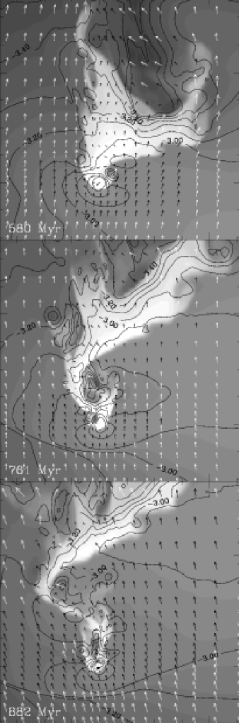
Figure 3: Gas density (grey scale at the bottom), pressure (black contour lines, logarithmically spaced from log$(p)$=-3.6 to log$(p)$=-2.6 in units of $10^{-24}$keV/cm³), and Mach vectors (arrows, drawn in white when Ma$>1$, and black otherwise) of model B. Coordinates are given in kpc. Numbers on the bottom left of each panel give elapsed time in Myr. A section in the plane of the orbit (panels on the left) and one in an orthogonal plane (panels on the right) are given for each time.

Gas-mass loss is largest in the part of the galaxy’s orbit near the pericentre where the kinetic force is largest. Its dynamics is regulated by the pressure distribution around the ISM produced by the supersonic flow. Rarefaction fans are formed at the rear of the galaxy at the same time as pressure builds up in front of it behind the bow shock. The presence of the bow shock itself contributes to the lateral pressure confinement of the ISM, while the ISM accelerates and expands where rarefaction fans form in the streaming ICM. As a result, the ISM is initially pushed back bodily, stretched and fanned out in the direction of motion. Figure 3 shows the evolution of model B during this phase. In contrast to the case of a body with a hard surface, no primary trailing shock is formed, because the ISM is free to expand. In time, K-H wiggles develop on the ISM-ICM interface, which produce secondary shocks and secondary rarefaction fans on the sides downstream of the galaxy centre. Irregular extensions or “tongues” of ISM form, which grow or stretch until they break away. The time scale of the whole process is intermediate between the dynamical crossing time and the sound crossing time for the cooler gas ($c_{s}\simeq 400$ km/s, as compared to $U_{G}\simeq 1200$ km/s).

The amount of ISM actually lost from the galaxy’s potential well depends on the kinetic pressure or momentum flux $\rho_{ICM}U_{G}^{2}$ and on how long it lasts. Stripping is boosted by rapidly growing K-H modes, but it is reduced by gas cooling and by counter streaming towards the centre of the galaxy from the rear (see also Nittmann et al. 1982). Condition (6) strictly applies only if ${\rm Ma}\gg 1$, since in that case one can neglect pressure forces acting on the ISM. For mildly transonic stripping, Eq. (6) is a sufficient condition for complete stripping only if it is valid in the centre of the galaxy and if it is satisfied over an ISM crossing time. If it is valid only outside a particular cylindrical radius, although that region will be depleted, it does not imply that all the ISM associated to it, which joins in the trail, will be lost in a dynamic time.

Initially, the momentum acquired by the ISM is spent in climbing up the galaxy’s potential well, so that for some time the ISM approximately co-moves with the galaxy. As soon as it is displaced and decelerated, it starts falling towards the cluster centre, since given a density ratio $T_{ICM}/T_{ISM}\sim 5$ its buoyancy in the ICM is small. The cluster gravitational force (or tidal force in the galaxy’s reference frame) is not small compared to the kinetic pressure force. A second shock is formed in front of the part of stripped, flowing material which is on the same side as the cluster centre with respect to the galaxy. The pressure built up behind the second shock in turn displaces the ISM upstream. This produces the “S”-shape of the trail visible in Fig. 3. The ISM nearer to the galaxy is subject to a pressure due to the large net momentum with respect to the galactic centre, which effectively “breaks” the trail and allows a flow of ISM towards the galactic centre. At the same time, other gas is stripped from the galaxy near the centre due to the growth of K-H wiggles, and the process may repeat on a smaller spatial scale.

In model B, at this point the galaxy is slowing down moving outwards from the cluster centre. No further stripping occurs after a second, minor event, and in the centre most of the ISM is retained. Moreover, the compression before the formation of the bow shock and after the formation of the lateral shock causes a reduction of the central cooling time and a net mass accretion in the centre. Despite ram pressure, a central cooling accretion flow is established. A similar situation obtains for model B$q$, where, however, significant mass loss continues also during subsonic motion due to the reduced density contrast. In models A1 and A2 kinetic pressure is large and prolonged enough to stop accretion and cause again heavy stripping. The rate of accumulation of ISM in the subsonic part of the orbit is crucial to determine the gas content at later stages.

4.2 Subsonic stripping flow

The growth of the ISM halo while the galaxy is moving towards its apocentre is regulated by gas accumulation via stellar gas injection. It increases the ISM density gradient near the centre and thus inhibits the linear growth of K-H modes. Balance is thus shifted toward gas accumulation at the ISM-ICM boundary, which proceeds faster than the entrainment of streaming gas. The boundary of the ISM halo, which is marked by a sharp density gradient, moves outwards until a point is reached where K-H stripping balances, on average, mass accumulation. Vortices are mainly created by non-linear K-H modes and, by growing in size, they entrain additional gas, until they are either ‘washed’ downstream or dissipated near the galaxy centre. The formation, advection and eventually dissipation of vortex structures thus traces events of abrupt loss or of more gradual capture of gas in the galactic gravitational potential well, which is related to significant mixing between the ISM and the ICM within the galaxy.

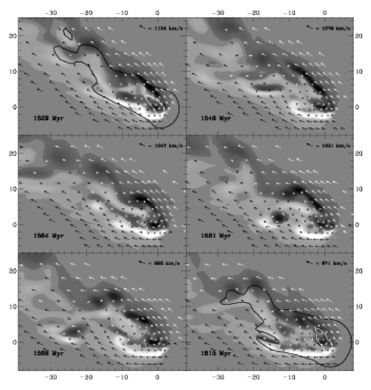
Figure 4: Velocity and vorticity field in the equatorial plane at 6 different times, at intervals of 17 Myr, for model A2. Arrows represent velocity vectors in the plane, while the background grey scale represents the corresponding z component of the vorticity field, from -0.61 (white) to 0.61 (black) Myr^-1. The time is given in each panel on the bottom left, the free-stream velocity of the ICM in the upper right corner. Lengths are given in kpc. The black contour lines in the first and in the last panel enclose the gas with negative binding energy density (kinetic plus potential); the white contours enclose the gas having negative total (binding plus thermal) energy density.

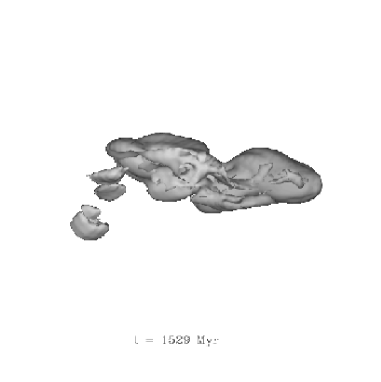
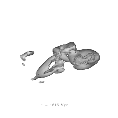
Figure 5: Three-dimensional view of the vorticity field for model A2. A surface of constant vorticity ($|\omega|=0.0165$ Myr^-1) is shown for two different times (as labelled). The size of the ring structure in the upper part of the right-hand side figure is about 5 kpc.

The velocity and vorticity fields during subsonic motion for model A2 are represented in Figs. 4 and 5. In Fig. 4, a cut in the equatorial plane of model A2 is shown, where the evolution and advection of vortices can be distinguished, while ISM is accumulating within the galaxy. In the present context, generation of vorticity is exclusively connected to stripping. Vorticity spreads as the size of the region of bound gas (black contour in Fig. 4) grows. Near the centre of the galaxy, the gas keeps concentrating, and smaller vortices develop. The complicated three-dimensional structure of the vorticity field, which tends to be organized in trailing filaments and rings as the gas-mass loss from the galaxy decreases, is visible in Fig. 5. While stripping is still substantial (t=1529 Myr, left, corresponding to the top left panel of Fig. 4), the vorticity field is more streamlined and distributed according to the stripped gas. Later, at t=1615 Myr, less regular structures appear, with an alternate shedding of vortex rings analogous to that occurring in 3-D aerodynamic flows past blunt bodies (Goldstein 1938, §250, p.577-579; Perry & Lim 1978).

Although the flow is only mildly subsonic, its character is very different from that of a case of ram-pressure stripping. The motion of the galaxy is communicated to an extended region of the ICM and kinetic pressure on the ISM is small. It is at this stage the necessity of a very wide computational grid (a half cube of 700 kpc size) becomes apparent. Comparison between the usual and the high-resolution (on a much smaller grid) computations we performed for cases A2 and B indicated consistency for the stripping rates.

Near the centre of the galaxy the ISM is rotating with angular momentum roughly aligned to the galaxy’s orbital angular momentum. The gas accreted has a net angular momentum in that direction. The flow round the galaxy in the equatorial plane has a non-zero circulation corresponding to an enhanced mass loss on the side of the galaxy opposite to the cluster centre (lower panel in Fig. 4), and enhanced accretion on the other side. In an orthogonal plane a similar situation may be attained but in certain regions and on short intervals of time only, the sign of the circulation changing frequently. The accretion region is much larger in model A1 than in model A2, where the flow pattern is even more complex and non-planar.

Figure 6: Richardson number $J$ (solid lines) and Mach number (dash-dotted line) as a function of time for model A2 (see Fig. 4). The thick solid line shows the value of the average $J$ over the high-vorticity region evidenced in Fig. 4 (defined to have a vorticity $|\omega|\geq 188$ km s^-1 kpc^-1). The thin solid line is the median of $J$ over that same region. The bottom part of the plot shows the minimum value of $J$ in the region considered.

An indication for the effectiveness of the K-H instability in determining the flow configuration is given by the value of the Richardson number (Figure 6), defined by

$$J\equiv\frac{\nabla\psi\cdot({\boldmath\omega}\times\mbox{\boldmath$u$})\>\nabla\ln(\rho)\cdot({\boldmath\omega}\times\mbox{\boldmath$u$})}{\omega^{2}|{\boldmath\omega}\times\mbox{\boldmath$u$}|^{2}}\,.$$ (28)

Incompressible K-H modes are stabilized when $J\raisebox{-4.2679pt}{$~{}\stackrel{{\scriptstyle\displaystyle>}}{{\sim}}~{}$}1/4$ locally (Chandrasekhar 1961, §103, p 491). Conversely, growing K-H modes are likely to exist as long as $J<1/4$, with wavelengths of the order of the scale given by the logarithmic density gradient (neglecting tidal forces: op. cit., §104). Compressibility, i.e. a free-stream Mach number Ma $\sim 1$, generally has a stabilizing effect. In our models we observe that the ‘noisy’ accretion phases correspond to average values of $J>1/4$, indicating that K-H modes are saturated. Locally, however, low values of $J$ are attained at all times, mainly as a result of mass injection via stellar mass loss.

4.3 Stripping and drop out

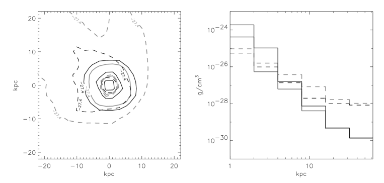
Figure 7: Left: Contours in the equatorial plane for the densities $\rho_{do}$ and $\rho$ (solid and dashed lines, respectively) for run B$q$, where $\rho_{do}$ represents the accumulated mass deposition per cm³. The gas is assumed to “freeze out” at the location of the reference system attached to the galaxy where it is lost from the normal gas phase. The distributions are given at $t=976$ Myr (grey lines) and $t=4055$ Myr (black lines), respectively. The contour levels of the decimal logarithm of the density in g/cm³ are -27.4, -25.7 and -24. Right: radial profiles from the spatial density distributions of the normal ISM and of that in drop-out form. Different line styles have the same meaning as the contour lines in the left panel.

Model B$q$ displays important deviations from the dynamics outlined above. From comparison of models B and B$q$ in Fig. 2, it is seen that drop out significantly affects the ISM content of the galaxy, and its dynamics. In general, a more nearly steady, self-regulated flow is achieved, having a lower density contrast between the gas near the centre of the galaxy and the ICM. Stripping is more continuous, but larger ISM mass-loss rates are obtained. The gas temperature undergoes smaller variations than in case B, and is generally higher as cold gas is dumped via drop out.

The drop-out rate is especially large when the ISM is bodily compressed while the galaxy is accelerated towards the pericentre. The reduced density contrast favours mass loss at intermediate radii in the subsonic stage. This further reduces the density contrast. As a consequence, less ISM is retained by the galaxy, either in gaseous or in drop-out form. Our quantitative results are sensitive to prescription (19) and to the value of $q$ adopted. However, the qualitative conclusion that drop out favours mass loss is robust.

In the specific case of model “B$q$”, with $q=0.4$, drop out occurs mostly in the centre of the galaxy, at such rate that after 4 Gyr the accumulated drop-out mass is $\sim$14 times larger than the ISM gas mass within a galactic half-luminosity radius ($r_{*}=16$ kpc). From Fig. 7 one can see that the mass distribution of gas dropped out of the flow keeps steepening as time passes. For $t>1$ Gyr, drop out is essentially confined to the central 20-30 kpc, with more of half the drop-out mass contained within 8 kpc. This regulates the radial profile of the ISM density, which, in contrast to what is observed in the other models, does not steepen as time passes. On the contrary, the central density even decreases.

In the subsonic phase, while a smaller density gradient allows a faster growth of K-H modes, the mass-loss term in Eq. (8) acts as an effective viscosity in the flow (Portnoy et al. 1993, Kritsuk et al. 1998). The K-H modes grow faster but saturate earlier. The saturated modes are associated with smaller mass flows also due to the lower ISM density. Thus, the mass-loss process is much smoother than in the non-drop-out models.

4.4 Secular evolution

The gas content of the model galaxies oscillates over a time equal to the radial period of the galaxy’s orbit, and heavy stripping alternates with replenishment and even cooling-driven accretion. The evolution, however, is not cyclic over the computed time interval, but shows rather a long-term tendency towards either complete cyclic stripping or a permanent cooling accretion flow onto the galaxy centre. In other words, no equilibrium between cooling and stripping and/or heating is achieved. Rather, in the central parts of the galaxy, one of the two processes eventually becomes ineffective. This is related mainly to the character of optically thin thermal radiative cooling (see also Kritsuk 1992), and to a lesser extent to the diminishing rate of gas replenishment from stars (Eq. (22)).

In model B, cooling is sufficient to start a central cooling accretion flow (essentially from the rear side) during the supersonic phase, gas accumulation/accretion is effective afterwards, and a further pericentre passage does not affect the ISM anymore. In model A2, ram pressure is large enough to strip the galaxy completely (if we consider only the gas having a negative total energy density). Model A1 is intermediate between the two, in that stripping affects the ISM also in the centre, but does not stop gas cooling which results in the formation of a central accretion flow in the subsonic part of the orbit. However, the next pericentre passage, 3 Gyr after “infall”, causes complete stripping.

Figure 8:       Secular evolution of the ISM content of the model elliptical galaxies. The thick lines represent for each model the total mass of the gas with negative total energy density in the galaxy’s reference frame. The thin smoother curves are fitted as described in the text (Eq. (30)).

We may attempt to quantify the long-term behaviour with an evolution equation for the ISM mass of the form

$$\frac{dM_{ISM}}{dt}\simeq\frac{\chi M_{ISM}}{\tau_{c0}}-\frac{\eta M_{ISM}\!(0)^{1+b}}{\tau_{orb}M_{ISM}^{b}}+\alpha_{*}M_{*}\left(\frac{\tau_{*}}{t}\right)^{1.3}\,,$$ (29)

where $\tau_{*}$ is the age of the stellar population of the galaxy, $\tau_{c0}$ the initial central cooling time, $\tau_{orb}$ the radial orbital period, $\alpha_{*}M_{*}$ the initial mass-injection rate, and $M_{ISM}(0)$ the initial ISM mass (intended here, as before, the total mass of gas with negative total energy density). The first term on the r.h.s. is related to cooling (with $\tau_{c}^{-1}\propto\rho$), the second to stripping, and the last is the mass injection. The mass dependence (or density dependence) through the parameter $b$ in the second term allows for the dependence of stripping efficiencies on the density contrast. If for simplicity we take $b=0$ and $\chi=1$, using $\dot{M}_{inj}\simeq M_{inj}(0)(1-1.3t/\tau_{*})$ we obtain

$$M_{ISM}\simeq M_{ISM}\!(0)+1.3\frac{\tau_{c0}}{\tau_{*}}M_{inj}\!(t)+$$ (30)

$$\left[M_{inj}\!(\tau_{c0})\left(1-0.65\frac{\tau_{c}}{\tau_{*}}\right)+M_{ISM}\!(0)\left(1-\eta\frac{\tau_{c0}}{\tau_{orb}}\right)\right]\left(\>{\rm e}^{t/\tau_{c0}}-1\right)\,.$$

Here, $\eta$ is a “fit” parameter characterizing the efficiency of stripping. If we add an oscillatory component to this estimate with a period equal to $\tau_{orb}$, a phase shift of a quarter period with respect to the orbital velocity, and a best fit amplitude, we find the fitting curves plotted in Fig. 8 together with the simulation data. The fitting curves clearly make sense only as long as the mass is positive. The values of $\eta$ appearing in Eq. 30 and of the amplitude $A$ of the sinusoidal components are given in Table 2.

	A1	A2	B	Bq
$M_{T}$	11	5.7	10	10
$\bar{m}$	1.23	1.23	0.95	0.95
$\bar{\sigma}$	1.31	1.31	0.15	0.15
$q$	0	0	0	0.4
$\eta$	4.20	4.25	2.56	3.67
$A$	2.6	1.4	0.25	1.6

Table 2: Fit parameters for the long-term evolution: total gravitational mass $M_{T}$ of the galaxy in units of $10^{11}{\rm M}_{\odot}$, time-averaged Mach number $\bar{m}$ of the galaxy velocity relative to the ICM, time-averaged incoming momentum flux $\bar{\sigma}$ of the ICM in the frame of the moving galaxy in units of $10^{-11}$ g cm^-2 s^-1, mass drop out parameter $q$, parameter characterizing the efficiency of stripping $\eta$ and amplitude of sinusoidal components $A$.

The fit, although corrected for drop out, is poor for model B$q$. The value for $\eta$, though, reflects the highly increased efficiency of stripping for this model as compared to its non-drop-out counterpart, model B.

In model B, as a result of the angular momentum acquired during stripping, the ISM cools onto a large central disk in the plane of the galactic orbit with a diameter of about 20 kpc, as shown in Fig. 9. The motion (essentially rotation) of the gas in the disk is supersonic, so that the disk is dynamically ‘cold’ with a temperature of 0.01 keV. The disk is warped and presents spiral arms which join a central bar-like structure lying in the plane of the disk and oriented perpendicularly to the motion of the galaxy. The gas flows towards the centre of the galaxy along the ‘bar’, which is very cold (0.001 keV, the lower limit allowed for in the computation) at a radius of $\sim 5$ kpc, but it is warmer in the centre because of the compression caused by infall. While some or all of the central infall may be artificial due to the resolution limits of the computation, the formation of the large disk structure seems inescapable.

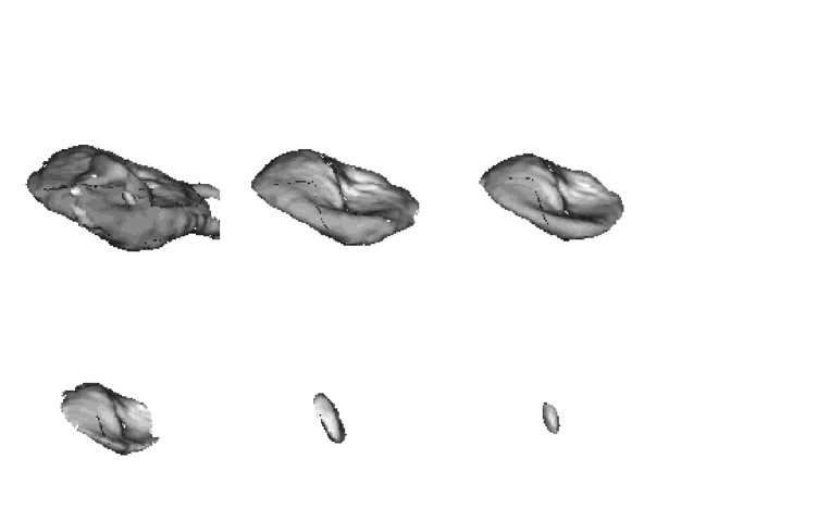
Figure 9: Disk-like ISM density distribution in model B at $t=$1870 Myr. Shown are surfaces of constant density. The six density levels, increasing from left to right and from top to bottom, are 8$\times 10^{-28}$, 3.2$\times 10^{-27}$, 1.28$\times 10^{-26}$, 5.12$\times 10^{-26}$, 2.05$\times 10^{-25}$, and 8.19$\times 10^{-25}$ g/cm³. On the bottom left the linear scale in kpc is given. The ICM streams by from the left.

5 Mass Loss and X-ray Emission

The ISM dynamics related to the stripping process has significant implications for the X-ray luminosity of the galaxy. In fact, we find that the continuous, but time-dependent stripping process studied in the present paper provides a possible explanation of the observed range of X-ray luminosities of large cluster ellipticals. Figure 10 shows the model luminosities of the four cases studied against the $L_{B}-L_{X}$ scatter plot obtained from X-ray data (Dow & White 1995; Brown & Bregman 1998).

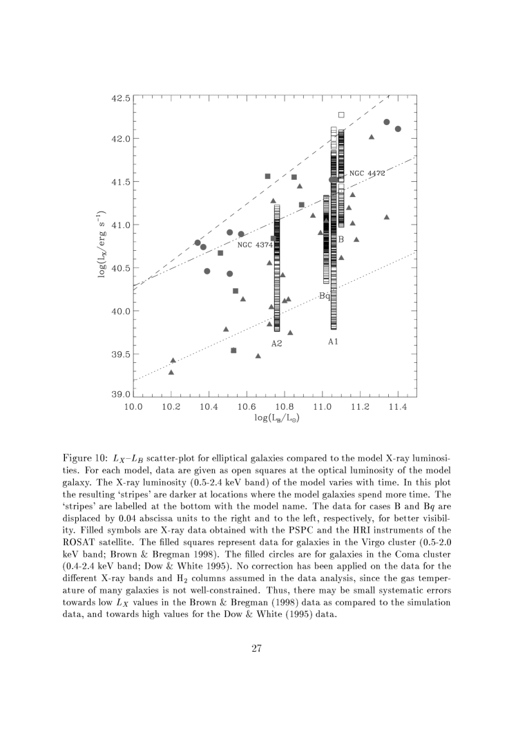
Figure 10: $L_{X}$–$L_{B}$ scatter plot for elliptical galaxies compared to the model X-ray luminosities. For each model, data are given as open squares at the optical luminosity of the model galaxy. The X-ray luminosity (0.5-2.4 keV band) of the model varies with time. In this plot the resulting ‘stripes’ are darker at locations where the model galaxies spend more time. The ‘stripes’ are labelled at the bottom with the model name. The data for cases B and B$q$ are displaced by 0.04 abscissa units to the right and to the left, respectively, for better visibility. Filled symbols are X-ray data obtained with the PSPC and the HRI instruments of the ROSAT satellite. The filled squares represent data for galaxies in the Virgo cluster (0.5-2.0 keV band; Brown & Bregman 1998). The filled circles are for galaxies in the Coma cluster (0.4-2.4 keV band; Dow & White 1995). No correction has been applied on the data for the different X-ray bands and H₂ columns assumed in the data analysis, since the gas temperature of many galaxies is not well constrained. Thus, there may be small systematic errors towards low $L_{X}$ values in the Brown & Bregman (1998) data as compared to the simulation data, and towards high values for the Dow & White (1995) data.

The same galaxy may display a widely different X-ray luminosity at different times, depending on the dynamic ‘phase’ the ISM is involved in (Fig. 11). Just after the large pericentric, supersonic (ram-pressure) stripping event, the X-ray luminosity is very small; while during the apocentric gas accumulation phase it rises to reach a maximum in response to the increasing external confinement just preceding a new pericentric ram-pressure stripping event. This correlation is evident in Fig. 11 especially for case A1. Case B, by contrast, is so accretion dominated that gas accumulation proceeds unchecked within the half-light radius of the galaxy, in spite of substantial stripping in the outer layers (see Fig. 3). Correspondingly, its X-ray luminosity rises continually as the ISM cools and concentrates onto the centre. Ongoing stripping mainly results in the large variability, over the scale of one crossing time, of the X-ray luminosity.

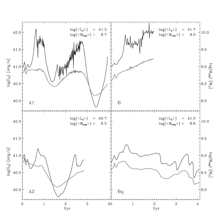
Figure 11: Gas-mass content and X-ray luminosity of the models as a function of time. Black lines refer to the X-ray luminosity in the 0.2-2.4 keV band; grey lines represent the ISM mass contained within the galactic half-light radius $R_{l}=16$ kpc. Model names are indicated on the bottom left of each panel; on the top right of each panel the time averages are given.

After sufficient time, due to what we have called a ‘secular’ evolution of the ISM, most galaxies will end up either completely stripped, like case A2, or hosting a cooling flow, like case B, with correspondingly widely different X-ray luminosity.

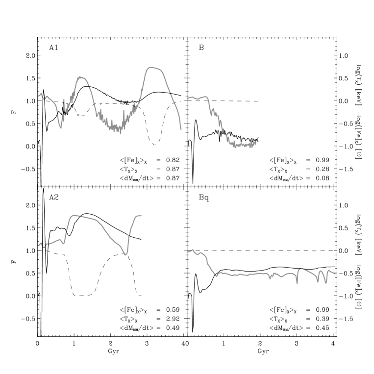
Figure 12: Stripping fraction and X-ray temperature of the models as a function of time. Solid black lines refer to the quantity $F$ defined as the ratio of the total gas-mass loss to the total injected gas mass. The scale is given on the left side. Thick grey lines represent the X-ray emission temperature (scale on the right). The dashed black lines are for the iron concentration in solar units. As in Fig. 11, the quantities refer to the region of the galaxy comprised within its optical half-light radius. On the bottom right of each panel the luminosity-weighted time averages of the emission temperature and of the iron abundance, as well as the average mass-loss rate are given.

The large scatter in X-ray luminosity between otherwise similar galaxies finds a natural interpretation in terms of a time evolution over a timescale of the order of the galaxy’s orbital period ($\sim$1 Gyr). The long-term evolution of the ISM halo (Section 4.4), on the other hand, which brings a galaxy either to be cyclically stripped or otherwise, takes several billion years. This time scale is small, but not entirely negligible compared to the evolutionary time scale of the cluster itself (Dressler & Shectman 1988).

X-ray temperatures correlate with the fraction of stellar ejecta lost from the galaxy. In Fig. 12 the quantity

$$F=\left[M(0)-M(t)+\int(\dot{M}_{inj}-\dot{M}_{do})dt\right]\mbox{\Large$/$}\int\dot{M}_{inj}dt$$ (31)

is shown. In a steady state, $F=1$. If $F>1$, the gas-mass content of the galaxy is decreasing, on average; if $F<1$, mass injection prevails and ISM is accumulating; $F<0$ indicates that net accretion has occurred. After an initial phase, for cases A1 and A2, which end up cyclically stripped, $F$ tends to unity. In case B, it tends to zero. Case Bq is intermediate, where part of the injected gas is lost, and part is retained, at least over a longer time scale. Correspondingly, also X-ray temperatures tend to range between extremes in the non-drop-out cases, and attain an intermediate value in case Bq.

Summarizing, model X-ray temperatures do not compare well with the data. Typical observed X-ray emission temperatures are about 1 keV. In the models, this temperature seems to be avoided. The ISM is either heated above the injection temperature in the case of efficient stripping, or it cools below it when stripping is inefficient. Case Bq does slightly better than the others, but the temperature is still too low, even for a relatively large value of $q$ (see Section 4.3). We comment on this inconsistency (see also Sect. 6.2) in the Conclusions (Sect. 8).

6 X-ray morphology

6.1 X-ray emission during supersonic stripping

The stage of ongoing supersonic stripping of the galaxy with its initial extended ISM halo lasts between 200 and 400 Myr, depending on the density of the ICM. The chances of observing such an event are therefore relatively small. However, a supersonic stripping process has often been related to the X-ray halo surrounding the Virgo elliptical NGC4406/M86 (e.g. Nulsen 1982; Rangarajan et al. 1995). This galaxy has a blue shift of 230 km/s, which added to the recession velocity of the Virgo cluster of 1150 km/s results in an estimated velocity of the galaxy relative to the ICM of 1380 km/s out along the line of sight. The galaxy’s total X-ray luminosity in the 0.1–2.4 keV band is $L_{X}\sim 4\times 10^{41}$ erg/s within a radius of 80 kpc, and the emission temperature is $T_{X}\simeq 0.8$ keV (Brown & Bregman 1998). The observed X-ray map is shown in Fig. 13 together with some synthetic maps from the simulations. Rangarajan et al. (1995) interpret the steep decline in the X-ray surface brightness on the north side of the galaxy as a possible Mach cone, and from its aperture derive an upper limit to the velocity component in the plane of the sky of 700 km/s. Combined with the approaching velocity reported above, an estimated streaming velocity of the ICM of $\sim 1550$ km/s in the frame of the galaxy is obtained.

     

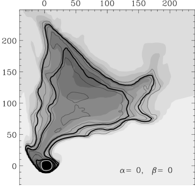
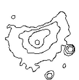
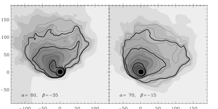
Figure 13: X-ray maps of model B at $t=579$ Myr in three different projection directions compared to ROSAT PSPC/HRI data for M86 (top right, from Rangarajan et al. 1995). PSPC data are represented by contour lines, HRI data by grey scales. Both observations – PSPC and HRI – and the models are to the same scale, the scale being given at the bottom and on the left. The model maps (upper left, and lower panels) give the temperature coded in grey scales (scale at the bottom of the Figure), and the X-ray surface brightness as contour levels, logarithmically spaced from -17.7 to -16.2 in units of erg s^-1 cm^-2 arcsec^-2. The thicker contours are directly comparable to those of the PSPC map. The quantities $\alpha$ and $\beta$ given at the bottom of each model projection are the polar angles of the projection direction in degrees.

The X-ray image of the M86 region has probably two major distinctive features which are thought to indicate ongoing stripping. One is the sharp decline in X-ray surface brightness on the north side, which makes the ROSAT/PSPC contour levels almost semi-circular. The other is the emission plume to the north-west of the emission maximum, best seen in the ROSAT/HRI data. The plume itself is very irregular and shows emission maxima and ‘holes’, as well as significant variation in the emission temperature (Rangarajan et al. 1995).

The model shown in Fig. 13, which is case B at $t=579$ Myr, has a total X-ray luminosity of $L_{X}=3.23\times 10^{41}$ erg/s, and an emission-weighted average emission temperature of $T_{X}=0.73$ keV, comparable to those observed for M86. The three projections result in apparent velocities in the plane of the sky of 1580, 1126 and 699 km/s, respectively, and apparent blue shifts with respect to the cluster of 0, 1109 and 1417 km/s, respectively. Thus especially the last projection may be suitable for a comparison. The synthetic X-ray surface-brightness distribution has an overall shape similar to that of the M86 region. However, neither ‘plume’ nor ‘edge’ are visible in this projection. Intrinsically, both features are present in the model, as is seen from the projection onto the equatorial plane. We are unable, though, to find a viewing direction from which both can be distinguished. The plume is quite prominent if the velocity in the plane of the sky is large; the rear edge of the ISM distribution, however, is evident only for very small relative blue shifts, and then the overall shape of the contours is triangular and not semicircular. When comparing the model maps to the data for M86, the coincidence of the X-ray centroid and the X-ray maximum in the latter becomes particularly puzzling. If the models under discussion are truly relevant for M86, we find that the Mach cone interpretation of Rangarajan et al. (1995) should be considered with some caution, allowing also for different possibilities. For instance, the edge may be the result of a strong inhomogeneity in the surrounding ICM. Also, the observed X-ray halo is probably related to a whole subcluster of $\sim$50 members rather than to M86 alone, resulting in a wider, possibly more irregular, potential well (Binggeli et al. 1993; Schindler et al. 1999).

A comparison with our models is still significant, though, because the gravitational potential and the gas sources near M86 should still be dominated by the giant elliptical.

Figure 13 gives some indication as to whether a detailed X-ray temperature map of an object like M86 would be helpful to determine its instantaneous motion relative to the ICM. We find that the synthetic X-ray temperature maps generally follow the X-ray surface-brightness maps, higher emissivities corresponding to colder gas. However, some remarkable deviation could be measured by an instrument sensitive to variation of 0.1 keV in temperature at $T\simeq 1$ keV. Specifically, the ‘plume’ in the $\alpha=60$, $\beta=-35$ projection is colder than the ‘surrounding’ gas, in projection. By comparison with the $\alpha=0$, $\beta=0$ map, it is seen that the gas visible in the plume is actually quite far away from the centre of the galaxy, and is cooler not as a result of radiative cooling but of the supersonic expansion of the stripped ISM downstream of the galaxy. Thus, an interpretation of the plume as of a ‘blob’ of freshly stripped gas, as opposed to that of the northern edge, would be misleading. From a single projection the kinematics of the ISM are not unambiguously identifiable.

In general, from our models we find that there is not necessarily an equivalence between the gradient in X-ray surface brightness, the pressure gradient, and the amount of ram pressure. The modelled ISM is not in equilibrium with the ambient pressure, but it expands (and even cools) while it is removed from the galaxy. Steep gradients in surface brightness partly arise from projection effects. Conversely, if the model is viewed in direction of the motion of the galaxy while it is subject to stripping, there is no obvious indication that stripping is occurring. From the synthetic X-ray maps one can work with the hypothesis that the gas is in hydrostatic equilibrium without meeting any evident inconsistencies, except for grossly misestimating the gravitational field of the galaxy.

6.2 X-ray surface-brightness profiles

Figure 14: Examples of azimuthally averaged radial X-ray emission profiles as derived from the models, compared with X-ray data of the elliptical galaxies NGC 4374 (triangles, Forman et al. 1985), NGC 4649 (diamonds, Trinchieri et al. 1997), and NGC 1404 (squares, Fabbiano et al. 1992), and of the lenticular galaxy NGC 1380 (crosses, Schlegel et al. 1998). The curves refer to the cases ‘A1’, ‘A2’, ‘B’, and ‘Bq’ as labelled, in projection onto the $x-z$ plane (except for case ‘B’ which is projected onto the $y-z$ plane), and at times $t=1972$, 1973, 1862 and 1868 Myr, respectively.

If the majority of cluster galaxies are subject to stripping, an important test of the present model is the comparison of typical surface brightness profiles of cluster galaxies with those obtained from the simulations. After a time of the order of the radial orbital period, when the outer ISM halo is subject to continuous stripping, the ISM distribution tends to become quite compact as a result of pressure confinement, continuous loss of gas from regions where the replenishment rate is small, and cooling. Viewed from a direction within $\pi/4$ of that of the velocity of the galaxy, the contours of constant X-ray surface brightness are fairly circular. Examples of azimuthally averaged emission profiles obtained for such cases are shown in Fig. 14 for all four models, and compared to the X-ray data of NGC 4374, NGC 4636, NGC 1404 and NGC 1380. The first two of these galaxies are Virgo cluster members, while the latter two are in the Fornax group dominated by NGC 1399. They represent cases in which ISM mass loss caused by gas dynamic interaction with the environment may have occurred.

Fig. 14 shows that the model profiles do not compare well with X-ray data. They are too steep, with most of the emission originating in the central 10 kpc. The inclusion of substantial drop out in case ‘Bq’, although making the emission more regular and more extended, does not significantly improve the fit to the data. Model ‘A2’ matches rather better at least the data of NGC 1380; the model total luminosity and the average emission temperature have values comparable to those of NGC 1380 ($L_{X}=3\times 10^{40}$ and $T_{X}\simeq 0.5$ keV). This result, though, is not robust, in that it depends on numerical implementation details and on the particular time chosen. Essentially, it appears that cooling of the gas in the centre of the galaxy is too efficient in the models. This is shown by computations with four times higher resolution in each spatial dimension performed for cases ‘B’ and ‘A2’. In spite of the large angular momentum of the ISM which tends to inhibit spherical central accretion, the profiles computed on the high-resolution grid are even more ‘bimodal’, with a distinct core of dense ISM.

In conclusion, the present models suffer from the same problem as ‘homogeneous’ steady-state cooling-flow models, namely the excess in central emission. This shortcoming is even increased by the stripping truncation of the ISM halo, which makes the emission profiles steeper overall, in such way that even the $q$-parameter drop-out prescription does not seem to be helpful.

7 Diluted ISM in the Cluster

7.1 Iron Enrichment and Distribution

The stripping of cluster galaxies causes the iron synthesized in SNIa events to mix with the ICM. Adopting the average stripping rate of our models after the first stripping, $\sim 1{\rm M}_{\odot}$/yr, we derive a net iron injection rate into the ICM of $\sim 0.2{\rm M}_{\odot}$/yr, if we assume a solar abundance in the ISM and a central density of 300 galaxies per Mpc³ within a core radius of $\sim 500$ kpc, like in Coma (Biviano et al. 1995). This figure doubles if $\sim 10$% of the galaxies in the cluster core are experiencing the stripping of an extended tenuous halo, like our models initially.

In young clusters, the ICM enrichment is even larger, because young stellar systems shed more gas to the environment (Eq. 22). In a computation for such case (model “C2” of Toniazzo 1998), in which the thermonuclear age of the galaxy was taken to be $\tau_{*}=3.44$ Gyr, the total amount of iron injected into the ICM over 2 Gyr was $\sim 6$ times as large as that of model A. Integrating the iron shed over $\tau_{*}=$1–15 Gyr under a ‘steady-stripping’ assumption, we derive a total mass of iron in the core of a Coma-like cluster of $1.3\times 10^{10}{\rm M}_{\odot}$ from galaxy stripping. For comparison, using the total gas mass and the gas density profile given by Reiprich (1998), and the metallicity given by Fukazawa et al. (1998) in the Coma cluster, the total amount of iron in the core ($R<500$kpc) is estimated to be $2.6\times 10^{10}{\rm M}_{\odot}$. Thus the standard scenario of stellar evolution, combined with the steady stripping of cluster galaxies plus a $\sim$10% of infalling objects, can explain the iron content of the ICM in a Coma-like cluster.

The injection rate of cool ISM into the ICM follows the number density of the cluster galaxies weighted by their stripping rate. Stripping mainly occurs while the galaxy is passing its orbital pericentre. Therefore, as opposed to a steady stripping process in which the ISM-shedding rate is constant and the iron enrichment follows the spatial distribution of galaxies, one can consider the case in which each galaxy deposits all gas stripped during one radial orbital period at the location of the orbital pericentre. The resulting radial density distribution of enriched material is proportional to the volume number density of cluster galaxies as a function of their pericentral distance, $n_{gp}(R_{p})$, defined in such a way that $n_{gp}(R_{p})4\pi R_{p}^{2}dR_{p}$ is the number of cluster galaxies which follow an orbit with a pericentre comprised between $R_{p}$ and $R_{p}+dR_{p}$. If the velocity distribution of the cluster galaxies is assumed to be isotropic and isothermal, and their spatial density is given by the function $n_{g}(R)$, where $R$ is the radial distance from the cluster centre, the function $n_{gp}(R_{p})$ is given by

$$n_{gp}=\int_{1}^{\infty}\left(1+z_{f}-z_{rp}\right){\rm e}^{-z_{f}/2y^{2}}\frac{yn_{g}(yx_{p})}{\sqrt{y^{2}-1}}dy\,,$$ (32)

where $x_{p}\equiv R_{p}/r_{C}$, $r_{C}$ is the cluster scale radius, $z_{f}=2y^{2}[\phi(yx_{p})-\phi(x_{p})]/(y^{2}-1)$, $z_{rp}=x_{p}d\phi(x_{p})/x_{p}$, and $\phi\equiv\Psi_{C}/\sigma_{C}^{2}$ is the cluster gravitational potential normalized to the (constant) one-dimensional velocity dispersion. The function $n_{gp}$ is shown in Fig. 15 for the example of the cluster mass distribution and cluster gravitational potential of Eq. (24), with $n_{g}(R)=1/(1+x^{2})^{3/2}$ and $x\equiv R/r_{C}$. The function $n_{gp}$ is steeper than $n_{g}$ and for $x<1$ it is $\sim 1/x$. These properties are very general and do not depend on the particular choice of the cluster density profile.

If the main source of iron enrichment of the ICM is actually due to the stripping of cluster galaxies, the function

$${\rm[Fe]}={\cal F}(R)=\frac{{\rm[Fe]}_{ICM}(1-S)\rho_{C}/\rho_{C0}+[Fe]_{ISM}Sn_{gp}(R/r_{C})/n_{g}(0)}{(1-S)\rho_{C}/\rho_{C0}+Sn_{gp}(R/r_{C})/n_{g}(0)}\,,$$ (33)

with the ‘unperturbed’ ICM density $\rho_{C}$ given e.g. by Eq. (26), will be proportional to the [Fe] abundance in the cluster gas. Here, $S$ is the ratio of the total gas mass of stripped material present in the ICM to the total ICM gas mass. The function ${\cal F}(R)$ is shown in Fig. 15 for the cluster model used for the calculations of model ‘A1’ and ‘A2’, and the parameters [Fe]_ICM=0.1, [Fe]_ISM=1, and $S=0.05$. In the same plot also the profiles are shown for the total mass fraction of iron within a given radius as a function of radius, and for the corresponding total X-ray emission weighted iron abundance. The occurrence of negative cluster metallicity gradients such as that shown in Fig. 15 is confirmed by recent X-ray observations as spatially resolved spectroscopic X-ray data become increasingly available (e.g. Molendi & De Grandi 1999).

Figure 15: Left: Number density of cluster galaxies normalized to the central number density (dotted line), the corresponding normalized pericentral density of stripped ISM (solid line), and the ICM density for the cluster mass distribution defined by Eqs. (24) and (26), normalized to the same total gas mass. The radial coordinate is in units of the cluster core radius $r_{C}$. A mixture of 95% “ICM” gas distribution and of 5% “stripped ISM” gas distribution is assumed. Right: abundance of iron in the cluster gas as obtained from Eq. (33) (solid line – see text), mass-weighted average iron abundance of the intracluster gas within a given radial distance (dash-dotted line), and emission-weighted average iron abundance of the ICM (dashed line).

7.2 Infall into the Cluster Centre

The inhomogeneous enrichment of the ICM by stripped material can have a further impact on the abundance distribution and also on the temperature of the cluster gas in the centre. With typical density ratios of 100-1000, the ISM lost from cluster galaxies will tend to fall inwards. We can argue that the mass flux involved in a ‘galaxy stripping induced inflow’, in which the diluted ISM resulting from cluster galaxy stripping falls into the centre of the cluster, is a monotonically increasing function of radial distance. The reason lies in the limited survival time of the stripped clouds.

The mass flux caused by the infall of stripped ISM clouds is

$$\dot{M}=4\pi R^{2}n_{gal}\Delta R\dot{M}_{st}\,,$$ (34)

where $R$ is the radial location in the cluster, $\dot{M}_{st}$ the mean gas mass stripping rate for a galaxy, and $\Delta R$ the average distance traveled by a cloud. The cloud is accelerated radially by $-(1-1/\tilde{r})d\Psi_{C}/dR$ for a time $\displaystyle t_{s}=F\frac{D}{\sigma_{C}}\sqrt{\tilde{r}}$, with $D$ the linear size of the cloud, $\tilde{r}=\rho_{ISM}/\rho_{ICM}$ and $F$ a factor of order unity. After a time $t_{s}$ the cloud is destroyed by the development of Rayleigh-Taylor instabilities (see e.g. Nittmann et al. 1982). Note that $\sigma_{C}$ is both the typical initial velocity of the cloud, and the sound speed of the hot ambient medium. The distance traveled by the cloud during the time $t_{s}$ is thus $\displaystyle\Delta R\simeq F^{2}D^{2}\left(\tilde{r}-1\right)\frac{R/r_{C}^{2}}{1+(R/r_{C})^{2}}$.

If we use the distribution of Eq. (32) for the cluster galaxies, by interpreting $R$ as the pericentre of the galaxy orbit, the resulting mass-flux profile, Eq. (34), is $\displaystyle\dot{M}(R)\simeq 4\pi F^{2}D^{2}(\tilde{r}-1)\dot{M}_{st}r_{C}x^{2}n_{gp}(x)/(1+x^{2})$, which is $\sim R^{2}$ in the centre, has a maximum near $R\simeq 0.8R_{C}$, and decreases as $1/R^{2}$ for $R>1$. The mass flux variation, however, is not associated with drop out but with actual accumulation of hot gas in the cluster centre. The radial divergence of $\dot{m}_{st}/R^{2}$ is proportional to $n_{gp}\sim 1/R$ for $R<r_{C}$. The ICM thus tends to accumulate in the cluster centre on a $1/R$ profile.

With $F\simeq 3$ (Nittmann et al. 1982), $r\simeq 10$, $D/r_{C}\simeq 0.01$, $\dot{M}_{st}\simeq 1{\rm M}_{\odot}/{\rm yr}$, and a total number of $\sim 10^{3}$ cluster galaxies within the cluster core radius, a maximum non-cooling inflow of $\sim 15{\rm M}_{\odot}$/yr is found at $R=0.79r_{C}$. Note that this value depends on the number of galaxies within the cluster core, and on the mean stripped ISM cloud size as well. The latter decreases with $\dot{M}_{st}$, since the size of the vortices determining the size of the stripped clouds is also smaller. Thus, a significant inflow rate occurs only in clusters in which large stripping events take place.

8 Summary and Concluding Remarks

We have studied the gas dynamic stripping of an elliptical galaxy orbiting in a cluster of galaxies for four cases (or “models”) by use of time dependent, three-dimensional, Eulerian, hydrodynamic numerical simulations. Accurate modeling of the galaxy, of its orbit, of the cluster background, and of the gas dynamics results in significantly reduced ISM mass-loss rates compared to previous calculations.

An initial state was chosen to represent a gas-filled galaxy which is entering the cluster on a rosette-shape orbit. The computation was continued until an unambiguous long-term evolution of the ISM halo was established for each case.

The gas dynamic evolution is different in different sections of the galaxy’s orbit. Near the pericentre, when the velocity of the galaxy is greater than the speed of sound in the ambient medium, ram pressure is effective. A major, sudden stripping ‘event’ can occur if the kinetic pressure grows rapidly to a value of the order of the central thermal pressure in the galaxy ($\sim 0.02$ keV cm^-3 for our models), and over a time comparable to or smaller than the sound crossing time of the ISM halo ($\sim 50$ Myr). Otherwise, stripping is more gradual.

Near the apocentre, where the orbital speed is slightly smaller than the speed of sound, the evolution is governed by gas-mass replenishment, radiative cooling, and the growth of Kelvin-Helmholtz modes. The latter result in the formation of eddies, that entrain streaming as well as galactic gas, and are eventually dragged away. This gives “impulsive” stripping alternated with short accretion phases. During this phase, mixing of the ISM and the ICM within the galaxy is significant.

Of the four cases studied, two (“A1” and “A2”) evolve, with different speeds, towards a cyclic “stripping replenishment” dynamics, in which stripping near the orbit’s pericentre is nearly complete, while a small ISM halo re-forms in the “upper” half of the orbit. In one case (“B”), cooling proceeds almost undisturbed and a “cooling flow” develops within the galaxy’s half-light radius, with the cooler gas distributed in a large disk of $\sim$20 kpc diameter. The angular momentum of the ISM is partly generated by ram-pressure torque in the supersonic phase, and partly by accreted orbital angular momentum in the subsonic phase.

The efficiency of the stripping process was estimated in terms of a dimensionless parameter, $\eta$, which gives the magnitude of the mass loss over a radial orbital period when linearly combined with cooling and replenishment to describe the long-term evolution of the gas-mass content of the galaxy. It appears that $\eta$ depends mainly on the orbit of the galaxy and on the cluster environment, and to a lesser extent on the total mass or the total optical luminosity of the galaxy.

The fourth model (“Bq”) was identical to model “B” except for the inclusion of mass drop out in the gas dynamic computations. The drop-out prescription adopted follows Sarazin & Ashe (1989) with $\dot{\rho}_{do}=q\rho/\tau_{c}$, $\tau_{c}$ being the cooling time and $q$ a dimensionless factor, which was taken to be $q=0.4$. It was found that drop out heavily affects the gas dynamics, causing enhanced total gas mass loss from the galaxy. Model “Bq” eventually approaches the cyclic stripping dynamics of models “A1” and “A2”, if on a much longer time scale.

The computed models account fully both for the observed correlation between optical and X-ray luminosities of cluster elliptical galaxies, and for its large dispersion. The X-ray luminosity of the gas associated with the model galaxies varies strongly depending on its orbit and on time. This time variation can produce for the same optical galaxy the whole range of X-ray luminosities observed. Due to the large gas dynamic energy input, stripping reduces the average X-ray luminosity $L_{X}$ of the ISM halo much less than its average mass. In this case drop out mainly reduces the range of $L_{X}$.

The X-ray morphology, luminosity and temperature of the models during the first, large stripping phase after “infall” are consistent with the X-ray data of the region surrounding the Virgo cluster elliptical M86, where gas dynamic stripping of an extended gaseous halo is taking place (Rangarajan et al. 1995). However, it was also found that after the ISM halo has suffered substantial truncation due to stripping, the computed X-ray temperatures and X-ray morphologies of the models are inconsistent with X-ray data of X-ray fainter cluster ellipticals, being generally too cool and too centrally concentrated. The inclusion of drop out does not improve the situation significantly.

We think that we are encountering here a difficulty inherent to the hydrodynamic treatment adopted, common also to steady-state, so-called homogeneous cooling flow models (e.g. Sarazin & White 1987), which have too steep X-ray profiles as compared to the data. It is known that the ISM is not thermally stable (Kritsuk 1992). In a quasi-hydrostatic, steady-state case, self-regulation can be achieved via the inclusion of a drop-out term (Kritsuk 1995). The $q$-prescription allows steady-state cooling flow models to match the observed X-ray surface brightness profiles (Bertin & Toniazzo 1995). The stripping process, however, results in a further concentration of the X-ray emission from the ISM, causing more intense cooling in the centre and heating in the outer part, thus destroying the approximate balance between radiative emission and SNIa heating of steady-state models. An even increased value of the parameter $q$ may partially solve the problem, at the price, however, of making stripping very effective, and thus of greatly reducing the gas-mass content and X-ray luminosity of a galaxy, to an extent which seems to be in disagreement with X-ray evidence on cluster galaxies.

Table 3 summarizes our main numerical results.

Model	A1	A2	B	B$q$
$\displaystyle M_{T}$${}^{~{}~{}(1)}$	11	5.7	10	10
$\displaystyle L_{B}$${}^{~{}~{}(2)}$	11	5.8	11	11
$\displaystyle\left(M_{g}\right)_{0}$${}^{~{}~{}(3)}$	24.2	20.7	25.6	25.6
$\displaystyle\tau_{c,0}$${}^{~{}~{}(4)}$	1.7	2.0	1.6	1.6
$\displaystyle\tau_{orb}$${}^{~{}~{}(5)}$	1.9	1.9	1.5	1.5
$\displaystyle\bar{m}$${}^{~{}~{}(6)}$	1.23	1.23	0.95	0.95
$\displaystyle\bar{\sigma}$${}^{~{}~{}(7)}$	1.31	1.31	0.15	0.15
$\displaystyle q$${}^{~{}~{}(8)}$	0	0	0	0.4
$\displaystyle\eta$${}^{~{}~{}(9)}$	4.2	4.3	2.6	3.7
$\displaystyle F$${}^{~{}~{}(10)}$	1.1	1.2	0.1	0.6
$\displaystyle\langle L_{X}\rangle$${}^{~{}~{}(11)}$	19.4	5.3	52.7	8.9
$\displaystyle\left(L_{X}\right)_{max}$${}^{~{}~{}(12)}$	126	15.8	188	20.4
$\displaystyle\left(L_{X}\right)_{min}$${}^{~{}~{}(13)}$	0.6	0.6	10	2.2
$\displaystyle\langle T_{X}\rangle$${}^{~{}~{}(14)}$	1.53	3.13	0.51	0.38
$\displaystyle\left(T_{X}\right)_{max}$${}^{~{}~{}(15)}$	5.39	5.87	1.22	1.03
$\displaystyle\left(T_{X}\right)_{min}$${}^{~{}~{}(16)}$	0.18	0.79	0.10	0.18
$\displaystyle\langle[{\rm Fe}]_{X}\rangle$${}^{~{}~{}(17)}$	0.72	0.52	0.99	0.98

Table 3: Main numerical results. ${}^{\,(1)}$: total gravitational mass of the galaxy in units of $10^{11}{\rm M}_{\odot}$.      ${}^{\,(2)}$: optical blue luminosity of the galaxy in units of $10^{10}{\rm L}_{\odot}$.      ${}^{\,(3)}$: total mass of the initial ISM gas distribution.      ${}^{\,(4)}$: central cooling time of the initial ISM gas distribution in Gyr..       ${}^{\,(5)}$: radial orbital period in Gyr.      ${}^{\,(6)}$: time-averaged Mach number of the galaxy velocity relative to the ICM.      ${}^{\,(7)}$: time-averaged incoming momentum flux of the ICM in the frame of the moving galaxy in units of $10^{-11}$ g cm^-2 s^-1.      ${}^{\,(8)}$: gas mass drop-out parameter.      ${}^{\,(9)}$: gas dynamic stripping efficiency parameter (Equation 30).      ${}^{\,(10)}$: Fractional stripping (Eq. 31).      ${}^{\,(11)}$: average ISM X-ray luminosity in units of $10^{40}$ erg/s.       ${}^{\,(12)}$: maximum ISM X-ray luminosity in units of $10^{40}$ erg/s.       ${}^{\,(13)}$: minimum ISM X-ray luminosity in units of $10^{40}$ erg/s.       ${}^{\,(14)}$: average ISM X-ray emission temperature in keV.      ${}^{\,(15)}$: maximum ISM X-ray emission temperature in keV.      ${}^{\,(16)}$: minimum ISM X-ray emission temperature in keV.      ${}^{\,(17)}$: average ISM emission-weighted iron abundance in solar units.     

Acknowledgements

This work is based on the results of the PhD Thesis of T. Toniazzo, carried out at the Max-Planck-Institut für Extraterrestrische Physik, Garching. T. Toniazzo wishes to express his gratitude to R. Treumann, whose supervision was extremely helpful, and to G. Bertin, for his continued support.

Many thanks to H. Böhringer and G. Morfill for their support, to E. Müller for providing a version of PROMETHEUS, to T.W.Hartquist for useful comments and to A. Shukurov for stimulating discussions. We thank the anonymous referee and Phil James for improving the presentation of the paper considerably.

This work was made possible by the excellent technical support provided by the Rechenzentrum of the Institut für Plasmaphysik, Garching, and by financial support from the Scuola Normale Superiore di Pisa, University of Trieste, and Deutscher Akademischer Austauschdienst.

References

• Abadi, M.G., Moore, B., & Bower, R.G., 1999, Monthly Not. of the Royal Astron. Soc. 308, 947

• Anders, E., & Grevesse, N., 1989, Geochim. Cosmochim Acta 53, 197

• Arnaud, M., Aghanim, N., Gastaud, R., Neumann, D.M., Lumb, D., et al., 2000, astro-ph/0011086

• Balsara, D., Livio, M., & O’Dea, C.P. 1994, Astrophys. J. 437, 83

• Bertin, G., Saglia, R.P., & Stiavelli, M., 1992, Astrophys. J. 384,423

• Bertin, G., & Toniazzo, T., 1995, Astrophys. J. 451, 111

• Binggeli, B., Popescu, C.C., & Tammann, G.A., 1993 Astron. & Astrophys. Supp. 98, 275

• Binney, J., & Tremaine, S., 1987, “Galactic dynamics”, Princeton University Press, Princeton 1987

• Biviano, A., Durret, F., Gerbal, D., Le Fevre, O., Lobo, C., Mazure, A., & Slezak, E., 1995, Astron. & Astrophys. Suppl. 111, 265

• Briel, U.G., Henry, J.P., & Böhringer, H., 1992, Astron. & Astrophys. 259, 31

• Brown, B.A., & Bregman, J.N., 1998, Astrophys. J., 495, L75

• Cappellaro, E., Turatto, M., Tsvetkov, D.Yu., Bartunov, O.S., Pollas, C., Evans, R., & Namuy, M. 1997, Astron. & Astrophys. 322, 431

• Chandrasekhar, S., 1961, “Hydrodynamic and hydromagnetic stability”, Clarendon Press, Oxford, 1961

• Ciotti, L., D’Ercole, A., Pellegrini, S., & Renzini, A., 1991, Astrophys. J. 376, 380

• Colella, P., & Woodward, P.R., 1984, J. Comput. Phys. 54, 174

• Colella, P., & Glaz, H.M., 1985, J. Comput. Phys. 59, 264

• Colless, M., & Dunn, A.M., 1996, Astrophys. J. 458, 435

• De Grandi, S., & Molendi, S., 2000, Astrophys. J., in press, astro-ph/0012232

• Dehnen, W., & Gerhard, O.E., 1994, Monthly Not. of the Royal Astron. Soc. 268, 1019

• Deiss, B.M., & Just, A., 1996, Astron. Astrophys. 305, 407

• Dow, K.L., & White, S.D.M., 1995, Astrophys. J. 439, 113

• Drake, N., Merrifield, M.R., Sakelliou, I., & Pinkney, J.C., 2000, Monthly Not. of the Royal Astron. Soc. 314, 768

• Dressler, A., & Shectman, S.A., 1988, Astronom. J. 95, 985

• Fabbiano, G., Kim, D.-W., & Trinchieri, G., 1992, Astrophys. J. Suppl. 80, 531

• Finoguenov, A., David, L.P., & Ponman, T.J., Astronomische Nachrichten 320, 286

• Forman, W., Jones, C., & Tucker, W., 1985, Astrophys. J. 293, 102

• Fryxell, B.A., Müller, E., & Arnett, D., 1989, MPA Report 449

• Fukazawa, Y., Makishima, K., Tamura, T., Ezawa, H., Xu, H., Ikebe, Y., Kikuchi, K., & Ohashi, T., 1998, Publ. of the Astron. Soc. of Japan 50, 187

• Gaetz, T.J., Salpeter, E.E., & Shaviv, G., 1987, Astrophys. J. 316, 530

• Gerhard, O., Jeske, G., Saglia, R.P., & Bender, R., 1998, Monthly Not. of the Royal Astron. Soc. 295, 197

• Godunov, S.K., Zabrodin, A.V., & Prokopov, G.P., 1961, U.S.S.R. Comput. Mathem. and Math. Physics 1, 1187

• Goldstein, S. (editor), 1938, Modern Developments in Fluid Dynamics, Fluid Motion Panel of the Aeronautical Research Committee, Clarendon Press, Oxford, 1938

• Gunn, J.E., & Gott, J.R., 1972, Astrophys. J. 176, 1

• Irwin, J.A., & Bregman, J.N., 2000, astro-ph/0009273

• Irwin, J.A., & Sarazin, C.L., 1998, Astrophys. J. 499, 650

• Jaffe, W., 1983, Monthly Not. of the Royal Astron. Soc. 202, 995

• Kritsuk, A.G., 1992, Astron. & Astrophys. 261, 78

• Kritsuk, A.G., 1995, Monthly Not. of the Royal Astron. Soc., 280, 319

• Kritsuk, A.G., Böhringer, H., & Müller, E., 1998, Monthly Not. of the Royal Astron. Soc. 301, 343

• Lea, S.M., & De Young, D.S., 1976, Astrophys. J. 210, 647

• Le Veque, R., “Nonlinear Conservation Laws and Finite Volume Methods for Astrophysical Fluid Flow”, in “Computational methods for astrophysical fluid flow. Saas Fee Advanced Course 27”, Lecture Notes 1997 of the Swiss Society for Astronomy and Astrophysics (SSAA), held March 3-8, 1997 in Les Diablerets, Switzerland. Edited by O. Steiner, and A. Gautschy. Publisher: Berlin, New York: Springer, 1998.

• Loewenstein, M., & Mathews, W.G., 1987, Astrophys. J. 319, 614

• Molendi, S., & de Grandi, S., 1999, Astron. & Astrophys. 351, L41

• Neumann, D.M., 1997, “Röntgenbeobachtungen von Galaxienhaufen und ihre Aussagen für die Kosmologie, PhD Thesis at the Ludwig-Maximilians Universität München.

• Nittmann, J., Falle, S.A.E.G., & Gaskell, P.H., 1982, Monthly Not. of the Royal Astron. Soc. 201, 833

• Nulsen, P.E.J., 1982, Monthly Not. of the Royal Astron. Soc. 198, 1007

• Perry, A.E., & Lim, T.T., 1978, J. Fluid Mech. 88, 451

• Portnoy, D., Pistinner, S., & Shaviv, G., 1993, Astrophys. J. Suppl. 86, 95

• Rangarajan, F.V.N., White, D.A., Ebeling, H., & Fabian, A.C., 1995, Monthly Not. of the Royal Astron. Soc. 277, 1047

• Reiprich, T.H., 1998, “Massenbestimmung an einer Stichprobe von Galaxienhaufen”, Diplomarbeit, Ludwig-Maximilians-Universität München

• Renzini, A., 1988, in Windows on Galaxies, Eds. G. Fabbiano, J.S. Ghallagher & A. Renzini, Dordrecht: Kluwer, p. 255

• Saglia, R.P., Bertin, G., & Stiavelli, M., 1992, Astrophys. J. 384,433

• Sarazin, C.L., & White, R.E., 1987, Astrophys. J. 320, 32

• Sarazin, C.L., & Ashe, G.A., 1989, Astrophys. J. 345, 22

• Schindler, S., Binggeli, B., Böhringer, H., 1999, Astron. & Astrophys. 343, 420

• Schipper, L., 1974, Monthly Not. of the Royal Astron. Soc. 168, 21

• Schlegel, E.M., Petre, R., & Loewenstein, M., 1998, Astronom. J. 115, 525

• Sutherland, R.S., & Dopita, M.A., 1993, Astrophys. J. Suppl. 88, 253

• Takeda H., Nulsen, P.E.J., & Fabian, A.C., 1984, Monthly Not. of the Royal Astron. Soc. 208, 261

• Toniazzo, T., 1998, “Hydrodynamical simulation of the X-ray emitting gas associated with cluster elliptical galaxies”, PhD Thesis, Technische Universität München

• Trinchieri, G., Noris, L., & di Serego Alighieri, S., 1997, Astron. & Astrophys. 326, 565

• Wheeler, J.C., Sneden, C., & Truran, J.W., 1989, Ann. Rev. A. A. 27, 279

• White, R.E., & Sarazin, C.L., 1991, Astrophys. J. 367, 476