Abundance Gradients and the Formation of the Milky Way

Abstract

In this paper we adopt a chemical evolution model, which is an improved version of the Chiappini, Matteucci, & Gratton (1997) model, assuming two main accretion episodes for the formation of the Galaxy: the first one forming the halo and bulge in a short timescale followed by a second one that forms the thin-disk, with a timescale which is an increasing function of the Galactocentric distance (being of the order of 7 Gyrs at the solar neighborhood). The present model takes into account in more detail than previously the halo density distribution and explores the effects of a threshold density in the star formation process, during both the halo and disk phases. The model also includes the most recent nucleosynthesis prescriptions concerning supernovae of all types, novae and single stars dying as white dwarfs. In the comparison between model predictions and available data, we have focused our attention on abundance gradients as well as gas, stellar and star formation rate distributions along the disk, since this kind of model has already proven to be quite successful in reproducing the solar neighborhood characteristics. We suggest that the mechanism for the formation of the halo leaves detectable imprints on the chemical properties of the outer regions of the disk, whereas the evolution of the halo and the inner disk are almost completely disentangled. This is due to the fact that the halo and disk densities are comparable at large Galactocentric distances and therefore the gas lost from the halo can substantially contribute to building up the outer disk. We also show that the existence of a threshold density for the star formation rate, both in the halo and disk phase, is necessary to reproduce the majority of observational data in the solar vicinity and in the whole disk. In particular, a threshold in the star formation implies the occurrence of a gap in the star formation at the halo-disk transition phase, in agreement with recent data.

We conclude that a relatively short halo formation timescale ($\simeq$ 0.8 Gyr), in agreement with recent estimates for the age differences among Galactic globular clusters, coupled with an “inside-out” formation of the Galactic disk, where the innermost regions are assumed to have formed much faster than the outermost ones, represents, at the moment, the most likely explanation for the formation of the Milky Way. This scenario allows us to predict abundance gradients and other radial properties of the Galactic disk in very good agreement with observations. Moreover, as a consequence of the adopted “inside-out” scenario for the disk, we predict that the abundance gradients along the Galactic disk must have increased with time and that the average $<[\alpha/$Fe$]>$ ratios in stars (halo plus disk) slightly decrease going from 4 to 10 kpcs from the Galactic centre. We also show that the same ratios increase substantially towards the outermost disk regions and the expected scatter in the stellar ages decreases, because the outermost regions are dominated by halo stars. More observations at large Galactocentric distances are needed to test these predictions.

1 INTRODUCTION

Most of the progress in understanding the formation and evolution of the Milky Way galaxy comes, on one side, from observations concerning chemical abundances in stars and gas and from the continuous improvement of stellar nucleosynthesis calculations on the other side. Other important quantities relevant to the chemical evolution of the Milky Way, such as the star formation rate (SFR), the initial mass function (IMF) and gas flows, are still poorly constrained. However, a good model of chemical evolution can allow us to impose constraints on such quantities. In particular, a good chemical evolution model should be able to reproduce observables larger in number than the number of adopted free parameters. Among the observables there are some which can help us to constrain the model better than others (see Matteucci 2000). The best observables from the point of view of Galactic chemical evolution are: the abundances in stars, in H II regions and planetary nebulae (PNe) from which we derive the abundance gradients along the Galactic disk, and the G-dwarf metallicity distribution in the solar neighborhood.

In past years a great deal of theoretical work has appeared concerning the chemical evolution of the Milky Way (Matteucci & François 1989; Carigi 1994, 1996; Timmes et al. 1995; Tsujimoto et al. 1995; Chiappini et al. 1997 (hereafter CMG97), 1999; Chang et al. 1999; Portinari & Chiosi 1999, 2000; Boissier & Prantzos 1999; Goswami & Prantzos 2000; Romano et al. 2000) and most of them dealt with the evolution of the Galactic disk only. Only a few models have attempted to model the Galactic halo (CMG97; Samland et al. 1997; Goswami & Prantzos 2000). In particular, CMG97 have suggested a scenario where the Galaxy forms as a result of two main infall episodes. During the first episode the halo forms and the gas lost by the halo rapidly (roughly 1 Gyr) accumulates in the center with the consequent formation of the bulge. During the second episode, a much slower infall of primordial gas gives rise to the disk with the gas accumulating faster in the inner than in the outer regions. In this scenario the formation of the halo and disk are almost completely dissociated although some halo gas falls into the disk. This mechanism for disk formation is known as “inside-out” scenario which is quite successful in reproducing the main features of the Milky Way (CMG97) as well as of external galaxies especially concerning abundance gradients (see Prantzos & Boissier, 2000).

In this paper we present a model similar to that of CMG97 and Romano et al. (2000) but with an improved treatment of the halo evolution. The model is always based on the “two-infall” scenario but more attention is paid to the evolution of the halo and to the possibility of a density threshold for the SFR in the halo. In the CMG97 paper we did not investigate in detail the effects of a density threshold for the star formation in the halo as our main goal was to study the solar neighborhood. Moreover, as will be shown in the next sections, the evolution of the solar neighborhood is almost independent of the enrichment history of the halo.

It is worth recalling that a surface density threshold for star formation has been observed in a variety of objects, including normal spirals, starburst galaxies and low surface brightness galaxies (e.g Kennicutt 1989, 1998; van der Hulst et al. 1993). The existence of a threshold in spheroidal systems (halos, bulges and ellipticals) is not yet clear although there are theoretical arguments by Elmegreen (1999) suggesting the existence of a threshold also in such systems. The threshold adopted by CMG97 produced results in very good agreement with the majority of the observational constraints in the solar neighborhood and in the whole disk. These include the most recent findings which suggest a discontinuity in the chemical properties between the halo (and part of the thick-disk) and the thin-disk (e.g. Pagel & Tautvaisiene 1995; Beers & Sommer-Larsen 1995; Gratton et al. 1996). In particular, one of the main effects of the threshold was that it naturally produced a hiatus in the SFR between the end of the halo/thick-disk phase and the beginning of the thin-disk phase. Such a hiatus seems to be real since it is observed both in the plot of [Fe/O] versus [O/H] (CMG97; Gratton et al. 1996, 2000; see also Pagel 2000 for a discussion) and in the plot of [Fe/Mg] versus [Mg/H] (Fuhrmann 1998; Gratton et al. 2000). The evidence for this is shown by the steep increase of [Fe/O] and [Fe/Mg] at a particular value of [O/H] and [Mg/H], respectively, indicating that at a certain epoch (coinciding with the halo-disk transition) SNe II, responsible for the production of O and Mg, stopped exploding while Fe, produced by the long living SNe Ia, continued to be produced. The star formation must have ceased for a period which cannot be longer than $\sim$ 1 Gyr, as suggested by theoretical models (CMG97; Gratton et al. 2000 and the present paper). The “two-infall” model also allowed us to fit the observed metallicity distribution of the G-dwarfs by assuming a long timescale for the thin-disk formation. This long timescale for the thin-disk formation at the solar vicinity was then suggested also by more recent chemical evolution models (e.g. Prantzos & Silk 1998; Portinari, Chiosi, & Bressan 1998; Chang et al. 1999; and more recently Boissier & Prantzos 1999; Hou et al. 2000). The same result is also suggested by chemodynamical models (Samland et al. 1997; Hensler 1999).

We not that in CMG97 we focused mainly on the solar vicinity modelling, and adopted very simplified assumptions to compute the radial profiles. We predicted non-linear gradients along the Galactic disk and a tendency for them to be flatter in the outermost regions and almost constant with time, whereas in the innermost parts they were steeper and steepened with time. In particular, the gradients we obtained were flatter than the standard values presently adopted in the literature. For example, the gradient of oxygen was flatter than $-$0.07 dex/kpc, which is the value suggested by different data sources (B stars, H II regions and PNe, see Maciel & Quireza 1999).

In this paper, we study in detail the formation of abundance gradients in the Galactic disk by trying to fit at the same time the abundance, SFR, star and gas profiles in the Milky Way (MW) disk. Clearly the evolution of gradients with time is strictly related to the mechanism of Galaxy formation, including the formation of the halo and this is an important point to assess. For this purpose, we test several assumptions about the halo and disk formation and the existence and variation of a density threshold for the SFR both in the halo and disk. Our results concern mostly the elements for which more data are available, such as N, O, S and Fe.

We believe that by improving the MW model we will provide a solid basis for a more detailed understanding of the history of chemical enrichment of our Galaxy and other spirals. An important aspect of this work will be to provide specific predictions for galaxy sizes of MW-like galaxies as a function of redshift type (in a forthcoming paper), which could in principle be tested against the growing body of observational data on distant galaxies. In particular, the slow timescale for the formation of the MW disk implied by our chemical evolution model implies that at high redshifts we should see smaller disks. Some observational tests, using the predictions of CMG97 with the growth of the thin-disk timescale as a function of Galactocentric distance, have already been done (Roche et al. 1998). Those authors estimate that galaxies at redshift 2 $<$ $z$ $<$ 3.5 show 2.79 $\pm$ 0.31 mag of surface brightness evolution relative to those at $z$ $<$ 0.35, which is significantly larger than the luminosity evolution over this redshift range. They suggest that this can be explained by a size and luminosity evolution model, in which the outer regions of spiral galaxies form later and with a longer timescale than the inner regions, causing the half-light radius to increase with time. Although the interpretation of the observational data is still controversial (see Simard et al. 1999), they clearly represent a powerful test for disk formation models.

The paper is organized as follows: in section 2 the observational constraints are discussed; section 3 presents the model assumptions and in section 4 the results are shown. Some conclusions are drawn in section 5.

2 OBSERVATIONAL DATA

2.1 Abundance gradients

Radial abundance profiles constitute one of the most important observational constraints for models of the evolution of the MW disk. However, over the past decade, different authors using different observational tools often came to contradictory views on both the shape, the magnitude and the evolution of the abundance gradients along the disk (see Tosi 1996, 2000 for a discussion on this point). The controversial results originate from both theoretical and observational considerations.

In particular, observations of B-stars seemed to rule out the existence of a gradient (or to allow for only a very mild one; Gehren et al. 1985; Fitzsimmons et al. 1992; Kaufer et al. 1994; Kilian-Montenbruck et al. 1994), in contrast to observations of H II regions (Shaver et al. 1983; Fich & Silkey 1991; Simpson et al. 1995; Afflerbach et al. 1997; Rudolph et al. 1997) and PNe of type II (Maciel & Chiappini 1994; Maciel & Köppen 1994; Maciel & Quireza 1999). This controversy was solved by Smartt & Rolleston (1997) and Gummersbach et al. (1998) who found, by means of the reanalysis of a sample of B-stars, a gradient similar to that derived from H II regions and PNe.

Although the B-star discrepancy seems now to be solved, a new one appeared recently in the literature concerning the H II regions abundance gradients. Deharveng et al. (2000) analysed a new sample of 34 H II regions located between 6.6 and 17.7 kpcs from the Galactic center and after a careful estimate of the electron temperatures in those objects they obtained, using their best observations, an oxygen abundance gradient which is flatter (by a factor of 2) than the one obtained in previous works based on H II regions. Their result seems to be in good agreement with results by Esteban et al. (1998, 1999a, b). Proposals for flatter gradients or bimodal ones have also been made by works based on open clusters (Friel 1999 and Twarog et al. 1997) although the situation is still very unclear (see Carraro et al. 1998). Observations of open clusters seem to support the existence of an iron gradient along the disk, but large uncertainties related to both the metallicity calibration and the ages of these objects are still present.

Another open question related to the observed abundance gradients concerns their variation with time: do the gradients steepen or flatten with time? This question cannot be answered properly by the presently available data (see Maciel 2000 for a discussion). However, PNe are the most promising objects to solve this problem. As has been extensively discussed in the past few years, PNe Galactic distribution, kinematics, chemical composition and morphology clearly indicate that PNe comprise objects of different populations (Peimbert 1978; Maciel 1997). Previous work has shown that disk objects of type II are particularly useful in tracing the chemical enrichment of the interstellar medium at the time of the formation of the PN progenitors (Maciel & Köppen 1994; Maciel & Chiappini 1994).

In a recent work, Maciel & Quireza (1999) obtained the gradients for a sample that includes the objects studied by Maciel & Köppen (1994), Maciel & Chiappini (1994) and Costa et al. (1997) (the latter consists of a sample of PNe near the anticentre direction intended to derive a better estimate of the gradients at Galactocentric distances larger than the solar position). Their main conclusions were: i) there is an average gradient of $-$0.04 to $-$0.07 dex/kpc for what they call “inner” Galaxy (between 4 and 10 kpc — those authors assume $R_{\odot}$ = 7.6 kpc); ii) the gradients show a small variation for the different element ratios (see their table 2); iii) the PN gradients are generally slightly flatter than those derived from younger objects; iv) for larger Galactocentric distances the PN gradients show some flattening. However the authors pointed out that a) the precise region where the gradient flattens out is not well defined and larger samples are needed, particularly at $R$ $>$ 12 kpc; and b) although the tendency of the gradients to steepen with time suggested by Maciel & Köppen (1994) seems to be confirmed by the more recent analysis, this is only an indicative result because of the difficulty of assigning precise ages to disk PNe and of estimating the importance of dynamical effects which could have flattened the gradients of the older objects.

From the theoretical point of view, several mechanisms have been proposed in order to explain the existence of abundance gradients in disk galaxies (see Matteucci & Chiappini 1999). Among the alternatives, the so called “biased-infall” is the most popular one. In this approach the Galactic disk formed by infall of gas occurring at a faster rate in the innermost regions than in the outermost ones (“inside-out” formation picture). The physical reason for a “biased-infall” can be found in the fact that the gas tends to collapse more quickly in the center of the spheroid so that a gradient in the gas density, lower in the more external parts, is established. In this situation the gas which continues to infall towards the disk falls more efficiently towards the center than towards the external regions, owing to the stronger tidal force acting at the center (see Larson 1976). Several authors have shown that the “biased-infall” can well reproduce the steep abundance gradients along the disk, especially if coupled with a SFR proportional to some power $k$ of the gas density (see section 3) with $k$ $>$ 1 (Tosi 1988; Matteucci & François 1989).

However, the situation is still not clear also from a theoretical point of view. In fact, as pointed out in many recent papers (Maciel & Quireza 1999; Tosi 2000; Portinari & Chiosi 2000; Deharveng et al. 2000; Hou et al. 2000 and others), different authors can fit the solar vicinity constraints and even the present time abundance gradients, but they seem to be divided into two groups concerning the evolution of the abundance gradients: in some of them the gradients steepen with time (Tosi 1988; CMG97; Samland et al. 1997) while in others the abundance gradients flatten with time (Allen et al. 1998; Portinari & Chiosi 2000; Hou et al. 2000). The lack of good data for the outer MW disk abundances still prevents us from testing this prediction and represents one of the main reasons for the non-uniqueness of the various chemical evolution models. Table 1 summarizes the abundance data available to trace the gradients in our Galaxy. In this work we present results for the Galactic abundance gradients of N, O, S and Fe as those are the elements for which more data exist.

2.2 Radial profiles

2.2.1 Gas

The observed (H I + H₂) distribution is taken from Dame (1993). The surface density distribution of the total gas $\Sigma_{gas}$ is obtained from the sum of the H I and H₂ distributions, $\Sigma_{HI}+\Sigma_{H_{2}}$, accounting for the helium and heavy elements fractions (thick line in figure 4).

2.2.2 Stars

The stellar profile is exponentially decreasing outwards, with characteristic scale length $R_{stars}$ $\sim$ 2.5 – 3 kpc (Sackett 1997 and references therein; Freudenreich 1998). Moreover, COBE observations suggest that the stellar disk has an outer edge 4 kpc from the Sun (Freudenreich 1998). To compare our model predictions on the stellar density profile along the Galactic disk to the observed one we consider $\Sigma_{stars}(R_{\odot},t_{Gal})$ = 35 $\pm$ 5 $M_{\odot}$ pc^-2 (Gilmore et al. 1989) and $R_{stars}$ = 2.5 kpc (see figure 5).

2.2.3 Star formation rate

The distributions of supernova remnants (Guibert, Lequeux, & Viallefond 1978), of pulsars (Lyne, Manchester, & Taylor 1985), of Lyman-continuum photons (Güsten & Mezger 1982) and of molecular gas (Rana 1991 and references therein) all can be used to derive an estimate for the SFR along the Galactic disk. Since these observables cannot directly yield the absolute SFR without further assumptions — e.g. on the IMF and mass ranges for producing pulsars, supernovae, etc. (see Lacey & Fall 1985), it is common practice to normalize them to their values at the solar radius, and then to trace the radial profile SFR($R$)/SFR($R_{\odot}$) (the thick lines plotted in figure 6 refer to the upper and lower limits obtained from the observational data listed above).

3 THE CHEMICAL EVOLUTION MODEL

As we stated in the introduction, a good model for the chemical evolution of our Galaxy should honour a minimal number of observational constraints both in the solar neighborhood and in the whole disk. The model we will adopt here is an updated version of the so called “two-infall” model of CMG97.

This model assumes that the Galaxy forms out of two main accretion episodes almost completely dissociated. During the first episode, the primordial gas collapses very quickly and forms the spheroidal components (halo and bulge); during the second episode, the thin-disk forms, mainly by accretion of a significant fraction of matter of primordial chemical composition plus traces of halo gas. The disk is built-up in the framework of the “inside-out” scenario of Galaxy formation (Larson 1976) which ensures the formation of abundance gradients along the disk (Matteucci & François 1989).

As in Matteucci & François (1989), the Galactic disk is approximated by several independent rings, 2 kpc wide, without exchange of matter between them. The rate of accretion of matter in each shell is:

$$\frac{d\Sigma_{I}(R,t)}{dt}=A(R)\,e^{-t/\tau_{H}}+B(R)\,e^{-(t-t_{max})/\tau_{D}},$$ (1)

where $\Sigma_{I}(R,t)$ is the surface mass density of the infalling material, which is assumed to have primordial chemical composition; $t_{max}$ is the time of maximum gas accretion onto the disk, coincident with the end of the halo/thick-disk phase and set here equal to 1 Gyr; $\tau_{H}$ and $\tau_{D}$ are the timescales for mass accretion onto the halo/thick-disk and thin-disk components, respectively. In particular, $\tau_{H}$ = 0.8 Gyr and, according to the “inside-out” scenario, $\tau_{D}(R)$ = 1.033$\times(R$/kpc)$-$1.267 Gyr (see Romano et al. 2000). We adopt a linear approximation for the variation of $\tau_{D}(R)$. However, this will be best constrained by the observed radial profiles of gas, SFR and abundances. In some cases the observed radial profiles suggest that this timescale can approach a constant value for Galactocentric distances larger than $\simeq$ 12 kpc (see next section). The quantities $A(R)$ and $B(R)$ are derived from the condition of reproducing the current total mass surface density distribution in the halo and along the disk respectively at the present time.

The SFR adopted here has the same formulation as in CMG97:

$$\psi(R,t)=\nu(t)\,\left(\frac{\Sigma(R,t)}{\Sigma(R_{\odot},t)}\right)^{2\,(k-1)}\,\left(\frac{\Sigma(R,t_{Gal})}{\Sigma(R,t)}\right)^{k-1}\,\Sigma_{gas}^{k}(R,t),$$ (2)

where $\nu(t)$ is the efficiency of the star formation process, $\Sigma(R,t)$ is the total mass surface density at a given radius $R$ and given time $t$, $\Sigma(R_{\odot},t)$ is the total mass surface density at the solar position and $\Sigma_{gas}(R,t)$ is the gas surface density. Note that the gas surface density exponent, $k$, equal to 1.5, was obtained from the best model of CMG97 in order to ensure a good fit to the observational constraints at the solar vicinity. This value is also in very good agreement with the recent observational results of Kennicutt (1998) and with N-body simulation results by Gerritsen & Icke (1997).

The efficiency of star formation is set to $\nu$=1 Gyr^-1 to ensure the best fit to the observational features in the solar vicinity, and becomes zero when the gas surface density drops below a certain critical threshold (Kennicutt 2000). We adopt a threshold density $\Sigma_{th}$ $\sim$ 7 $M_{\odot}$ pc^-2 in the disk (CMG97). As far as the halo/thick-disk phase is concerned, a similar value for the threshold is expected (see Elmegreen 1999 and the Model A description below for details).

The IMF is that of Scalo (1986), assumed to be constant during the evolution of the Galaxy (see Chiappini, Matteucci & Padoan 2000). Our present model differs from that of CMG97 in (i) the adopted yields for the low and intermediate mass range stars which are now taken from van den Hoek & Groenewegen (1997) instead of Renzini & Voli (1981) (see Romano et al. 2000); (ii) the fact that now we are including the explosive nucleosynthesis from nova outbursts (see Romano & Matteucci 2000) and (iii) the adopted solar Galactocentric distance ($R_{\odot}$ = 8 $\pm$ 0.5 kpc, Reid 1993) and age of the Galaxy ($t_{Gal}$ = 14 Gyr). Moreover, in the present model we adopt a primordial ⁴He abundance of 0.241 (by mass) instead of 0.23 as recently suggested by Viegas, Gruenwald, & Steigman (2000). The primordial abundances by mass of D and ³He were taken to be 4.5 $\times$ 10^-5 and 2.0 $\times$ 10^-5 respectively (see Chiappini & Matteucci 2000).

We run several models by varying the SFR threshold in the halo phase, the surface mass density distribution of the halo and the timescale for the halo formation. The present surface mass density distribution of the disk has been always kept the same and is exponential with scale length $R_{D}$ = 3.5 kpc normalized to $\Sigma_{D}(R_{\odot},t_{Gal})$ = 54 $M_{\odot}$ pc^-2 (see Romano et al. 2000 for a discussion of the choice of these parameters).

The models are labelled A, B, C, D and the model parameters are summarized in Table 5.

In particular, Model A assumes:

$\bullet$ the total halo mass density profile is constant and equal to 17 $M_{\odot}$ pc^-2 for $R$ $\leq$ 8 kpc and decreases as $R^{-1}$ outwards. We adopt the halo mass profile given by Binney & Tremaine (1987) where the density is proportional to $R^{-2}$ and this implies a surface mass density profile proportional to $R^{-1}$; the value of the total surface mass density of the halo at the solar position is quite uncertain, and we assumed it to be 17 $M_{\odot}$ pc^-2 from the fact that the total surface mass density (halo plus disk) in the solar vicinity is $\simeq$ 71 $M_{\odot}$ pc^-2 (Kuijken and Gilmore 1991), where $\simeq$ 54 $M_{\odot}$ pc^-2 corresponds to the disk total surface mass density (see also a discussion in Romano et al. 2000).

$\bullet$ $\tau_{H}$ is constant and equal to 0.8 Gyr along the overall Galactic disk, and $\tau_{D}(R)$ is an increasing function of $R$ in the range 4 – 14 kpc, as described above, and constant and equal to $\tau_{D}$(14 kpc) for $R$ $>$ 14 kpc.

$\bullet$ the thresholds in the gas density are 4 and 7 $M_{\odot}$ pc^-2 during the halo and disk phase, respectively. These choices are not arbitrary since the threshold for the disk agrees with the observational values found by Kennicutt (1989, 1998). Not much is known about the threshold in the halo and so this particular choice is a result of several tests and ensures a good fit to the main observational constraints. In particular, these choices for the density thresholds lead to a very good fit of the gap in the SFR during the halo-disk transition phase, as suggested by both the [Fe/O] vs. [O/H] and [Fe/Mg] vs. [Mg/H] relations, as well as of the radial profiles in the disk.

A possible physical motivation for different star formation thresholds in the halo and the disk might be related to a metallicity effect. Since the opacities are lower in the halo due to a lower metal content, this would make it easier for a protostellar cloud to cool and collapse and in this case we would expect a lower threshold density. Moreover, if the threshold density is close to the tidal limit (which is the average total density inside a radius R), then it would be higher in the inner regions than in the outer ones. Consequently one would expect a higher threshold density in the bulge than in the disk outside the bulge and higher in the disk than in the remote halo that is further out from the center (Elmegreen 1999). However, it is worth nothing that in the present model we adopt a simplification of the problem as both the disk and halo threshold density are taken as constant with the galactocentric distance. A more physical treatment of the threshold (varying with position) will be pursued in a forthcoming paper.

Model B assumes that:

$\bullet$ same as Model A, but considering a constant halo surface mass density of $\Sigma_{H}(R,t_{Gal})$ = 17 $M_{\odot}$ pc^-2 at all Galactocentric distances.

Model C assumes that:

$\bullet$ same as Model A, but no threshold in the gas density during the halo/thick-disk phase.

Finally, Model D assumes that:

$\bullet$ same as Model A, but also $\tau_{H}$ varies as a function of $R$: $\tau_{H}(R)$ = 0.8 Gyr for $R$ $\leq$ 10 Gyr, $\tau_{H}(R)$ = 2 Gyr for $R$ $\geq$ 12 Gyr. This slower formation of the outer halo might represent a merging scenario for the halo formation as originally suggested by Searle & Zinn (1978). In other words this simulates an “inside-out” formation also for the halo. The situation, in this case, is similar to that predicted by models which do not take the halo into account in studying the formation of the disk (e.g. Boissier & Prantzos 1999; Portinari & Chiosi 1999, 2000). These models predict steep abundance gradients in the outermost disk regions owing to the fact that they do not take into account the pre-enrichment of the disk due to the halo, which is not negligible at large Galactocentric distances.

4 MODEL RESULTS

4.1 The solar vicinity

All the above models can fit the available constraints in the solar vicinity (see table 2), however they differ substantially in reproducing the properties of the whole disk. In particular, concerning the solar neighborhood, our models are in good agreement with what is called the minimum set of observational constraints, among which the most important is the G-dwarf metallicity distribution (see Tosi 2000 for a recent review; see figure 1 for Model A). In table 3 we present the values for the observables in the solar vicinity predicted by Models A and C (the results from Models B and D are the same as Model A for the solar vicinity and they differ only for $R$ $>$ 8 kpc). In table 4 we show the solar abundances predicted by Model A compared to the observed ones (Anders & Grevesse 1989; Grevesse & Sauval 1998) and the agreement is quite good. Model C gives almost the same predictions as Model A concerning solar abundances, so we do not list them here. This is because at the solar radius the chemical evolution of the thin-disk is not influenced by that of the halo/thick-disk. On the contrary, the abundances observed at the outermost radii strongly reflect the chemical enrichment occurring during the halo phase, as we will see in the next section.

It is worth noting that all of these models provide a good fit of the [$\alpha$/Fe] versus [Fe/H] relation in the solar vicinity, as shown in Chiappini et al. (1999). Here we only show the plot of [Fe/O] versus [O/H] which indicates the existence of a gap in the SFR occurring at [O/H] $\sim$ $-$0.2 dex (see figure 2a). In fact, if there is a gap in the SFR we should expect both a steep increase of [Fe/O] at a fixed [O/H] and a lack of stars corresponding to the gap period. This is what both our model (Model A) and the data show. This gap, suggested also by the [Fe/Mg] data of Fuhrmann (1998), in our models is due to the adoption of the threshold in the star formation process coupled with the assumption of a slow infall for the formation of the disk. This is evident from figure 3 which shows clearly a halt in the SFR at the halo-disk transition. A similar explanation for the gap in the star formation rate is that it might result from the fact that the star formation in the halo begins while the protogalaxy is still in an overall expansion phase. Consequently the disk can only form later as the protogalaxy collapses and virializes (see Mathews and Schramm 1993).

It is worth noting here, that the data in figure 2a belong to a large compilation presented in Gratton et al. (2000). These data contain abundances obtained both from permitted and forbidden lines and do not show the linear decrease in [Fe/O] (or the growth in [O/Fe]) for low metallicity exhibited by recent data from Israelian et al. (1998) and Boesgaard et al. (1999) obtained from UV OH lines. This oxygen abundance controversy is particularly embarassing from a theoretical point of view, since a steep increase of [O/Fe] at low metallicities would imply the same behaviour also for the other $\alpha$-elements (but see Ramaty et al. 2000 for a solution involving only oxygen), and this, it seems, is not observed.

If such behaviour is confirmed also for the other $\alpha$- elements (sharing a common origin with oxygen) we should revise the yields of Fe and/or those of oxygen. In fact, a linear increase of the [O/Fe] could be due either to a lower contribution of Fe from type II SNe or to a metallicity dependent yield of oxygen or, as a last possibility, to a strong variation of the IMF during the halo phase. An earlier appearance of type Ia SNe during the halo phase (at around [Fe/H] = $-$3.0) is unrealistic since it would imply that stars more massive than 8 $M_{\odot}$ can be progenitors of such supernovae. In fact, most of the models in the literature (including the present one) do not produce the observed linear behaviour of the [Fe/O] found by Israelian et al. (1998), although those models assume an 8 $M_{\odot}$ star as the maximum mass allowed to form a CO white dwarf, corresponding to a timescale of only about 300 Myr for the first explosions. However, it is worth noting that although the first type Ia SNe may occur quite early, the bulk of them occurs only after $\sim$ 1 Gyr (Matteucci & Greggio 1986) and produce a visible change in the abundance ratios for metallicities larger than [Fe/H] $\simeq$ $-$1. Recent SN Ia models with maximum allowed progenitors smaller than 8 $M_{\odot}$ have been suggested, but the chemical evolution results seem to be unaffected (Kobayashi et al. 1999), thus confirming that only the SN Ia originating from low mass stars have an impact on the abundances of the ISM. The small increase of [O/Fe] for [Fe/H] $<$ $-1$ is far from being the observed trend by Israelian et al. (1998), contrary to what is stated by Goswami & Prantzos (2000). As explained in Chiappini et al. (1999) the reason why the so-called “[O/Fe]-plateau” is not exactly flat is due to a) the fact that some contribution by SN Ia can happen already after about 300 Myr as explained above and b) the fact that the stellar evolution calculations for massive stars (Woosley & Weaver 1995; Thielemann et al. 1996) predict that the ejected mass of (O/Fe)_ej by a massive star is an increasing function of the stellar mass (see figure 2b).

4.2 Radial profiles: does the halo evolution modify the abundance gradients?

Our results for the radial profiles of gas, stars and SFR are shown in figures 4, 5 and 6, respectively. It can be seen that Model A is the model in best agreement with the observations. Model B (constant halo density profile) overestimates the star density in the outer regions while Model D underestimates this quantity. Moreover, Model B gives a constant gas profile for Galactocentric distances between 8 – 20 kpc, at variance with observations.

In figures 7, 8 and 9 we compare the model predictions with the abundance data for N, O and S, respectively. In the upper panels the present time gradient is shown: our model predictions are compared with abundance data obtained from H II regions and B-stars (see section 2). In the lower panels a comparison is made with data from PNe of type II (roughly 2 Gyrs old objects). In figure 10 the abundance data on open clusters are compared with our model predictions for the present day abundance gradient. We did not attempt to separate the open cluster sample by age.

Among all the gradient figures, Model A seems again to be the one which best agrees with the observations. Model B predicts gradients that are flatter than the observed ones (as in CMG97), while Model D predicts too steep gradients.

Model C is instead an alternative model which could be supported by the observations. In fact, given the scatter of the observations for a given Galactocentric distance, it is very difficult to constrain our models, especially in the outer parts of the disk. Model C assumes no density threshold for the SFR in the halo phase. As a consequence, a higher initial level of enrichment due to the halo evolution is reached in the Galactic disk, which is almost constant for Galactocentric distances larger than 12 kpc (see also the almost constant stellar profile predicted by this model in figure 5). This is due to the predominance of the halo gas in the outer regions of the disk and it creates a pre-enriched disk gas dominating the subsequently accreted primordial one.

Figure 11 shows the behaviour of the abundance gradients, for each element and each model, at four different epochs of the evolution of the Galaxy. In figure 12 we show the abundance gradient behaviour as a function of time (between 4 and 14 kpcs). As is clearly shown by this figure the inner gradients tend to steepen with time while the outer gradients remain essentially constant. This conclusion is in agreement with CMG97 and with the chemodynamical model results (Samland et al. 1997). This behaviour is expected in a model taking into account the “inside-out” formation of the disk, where the external disk regions are still forming now and the abundance gradient is still building up. In fact, at early epochs, the efficiency in the chemical enrichment of the inner Galactic regions is low (due to the large amount of primordial infalling gas) leading to a flat initial abundance gradient. Then, at late epochs, while the SFR is still much higher in the central than in the external regions the infall of metal poor gas is stronger in the outer than in the inner regions, thus steepening the gradients.

However, other authors find a flattening of the gradients (see Tosi 2000 for a clear discussion on the possible scenarios for the evolution of the abundance gradients). A flattening of the gradients with time can clearly be achieved if one assumes that the disk formed on the same timescale at any Galactocentric distance, but with this scenario it is very difficult to reproduce the correct gradients at the present time. However, models adopting the “inside-out” picture for the disk formation also seem to create gradients flattening with time. This can be explained as follows: in the inner parts of the disk those models assume a very high efficiency in the chemical enrichment process already in the earliest phases of the Galaxy evolution, thus soon reaching a maximum metallicity in the gas which then remains constant or decreases due to the gas recycled by dying stars (Portinari & Chiosi 1999; Hou et al. 2000; Boissier & Prantzos 1999). At the same time, in the outermost disk regions the lack of any pre-enrichment from the halo phase (a similar situation is shown by our model D discussed above) and the fact that those models do not include a threshold in the star formation process in the disk, produces a growth of metallicity which we do not find. This also explains an important difference between the results shown in our figure 11 and those of figure 4 of Hou et al. (2000). As in their model the halo phase is completely decoupled from the disk evolution (even in the outer parts), their initial metallicities at larger Galactocentric distances are very small. Moreover, since they do not consider a threshold on the star formation process in the disk, their predicted abundances in the outermost parts of the disk keep increasing with time leading to a flattening of the abundance gradients.

In summary, from figure 12 we can conclude that:

a) Model B gives the flattest gradients. This model is in good agreement with the recent flatter gradient suggested by Deharveng et al. (2000). The predicted gas and stellar density profiles are at variance with the observed ones in the outer parts of the disk. However, we stress that large uncertainties are still present in the observed profiles especially at larger Galactocentric distances.

b) Model C predicts a present time gradient of O in agreement with the “standard” adopted value of $-$0.07 to $-$0.06 dex/kpc as suggested by B-stars, PNe and most of the data based on H II regions. Morever, it predicts a steeper gradient for Fe and N than for O and S, which is in agreement for instance with the results by Shaver et al. (1983) (see table 1) where a gradient of $-$0.07 dex/kpc is measured for oxygen while a value of $-$0.09 dex/kpc is obtained for N. The fact that the N gradient is steeper than the O gradient is not surprising since N is mainly a secondary element (i.e. its abundance is metallicity dependent) and is mainly produced on long timescales as is iron.

c) Model A also predicts gradients that steepen with time but only in the first 5 Gyrs of the Galactic disk evolution, remaining essentially constant with time after that. Again the gradients obtained for O and S are flatter than the ones obtained for N and Fe. The abundance gradients obtained in Model A for the present time are slightly flatter than the ones of Model C (for a Galactocentric range of 4 – 14 kpc).

Finally, in figure 13 we show the predicted $<$[O/Fe]$>$ ratios in the stars born and still alive at any Galactocentric distance (including halo, thick- and thin-disk stars) as a function of such distance. In particular, this ratio refers to the stellar population dominating in mass at any radius. It is clear from the figure that, while the ratios are slightly decreasing in the Galactocentric distance range 4 – 10 kpcs, as expected from the “inside-out” disk formation, they substantially increase at large radii. This is due to the fact that for $R>10$ kpcs the halo/thick-disk stars are dominating and they have large [O/Fe] ratios. In the same figure we show also the plot of the same ratios versus the stellar age of the dominating stellar population and this confirms that the stars dominating in the outermost disk regions are the oldest ones. This also means that the spread in stellar ages is a decreasing function of the Galactocentric distance. Edvardsson (1998) showed similar plots but only for disk stars older than 10 Gyrs and located between 4 and 14 kpcs and, although a precise comparison cannot be made, they seem to be in agreement with our predictions.

4.2.1 Radial profiles: main results

$\bullet$ The outer gradients are sensitive to the halo evolution, in particular to the amount of halo gas which ends up in the disk. This result is not surprising since the halo density is comparable to that of the outer disk, whereas it is negligible when compared to that of the inner disk. Therefore, the inner parts of the disk ($R$ $<$ $R_{\odot}$) evolve independently from the halo evolution in agreement with CMG97 result.

$\bullet$ Our best-model predicts gradients in good agreement with the observed ones in PNe, H II regions and open clusters. In CMG97 we found flatter gradients than in the present paper and in Matteucci & François (1989), although a very similar “inside-out” scenario was assumed in all these papers. The reason for being flatter than in Matteucci & François (1989) results from the fact that in CMG97 we adopted a threshold density for the SFR. This means that every time the gas density goes below the threshold then the star formation stops and starts again only after the gas has reached a density above the threshold, because of new infalling gas and/or the gas restored by dying stars (see figure 3). In particular, the effect of such a threshold was to keep the gas density always close to the threshold value especially at late times and large radii, thus contributing to maintaining an almost constant metallicity irrespective of the Galactocentric distance. The reason for the fact that the present model predicts steeper gradients than CMG97, although a threshold is also assumed, is that we considered here a more realistic halo density distribution, namely, a decreasing function of the galactocentric distance for $R>$ 8kpc, leading to a smaller contribution of the halo to the disk component metallicity enrichment at large radii.

$\bullet$ We predict that the abundance gradients along the Galactic disk must have increased with time. This is a direct consequence of the assumed “inside-out” scenario for the formation of the Galactic disk. Moreover, the gradients of different elements are predicted to be slightly different, owing to their different nucleosynthesis histories. In particular, Fe and N, which are produced on longer timescales than the $\alpha$-elements, show steeper gradients. Unfortunately, the available observations cannot yet confirm or disprove this, because the predicted differences are below the limit of detectability.

$\bullet$ Our model demonstrates a satisfactory fit to the elemental abundance gradients and it is also in good agreement with the observed radial profiles of the SFR, gas density and the number of stars in the disk.

$\bullet$ Our best model suggests that the average $<[\alpha/$Fe]$>$ ratio in stars slightly decreases from 4 to 10 kpcs. This is due to the predominance of disk over halo stars in this distance range and to the fact that the “inside-out” scenario for the disk predicts a decrease of such ratios (Matteucci 1991). On the other hand we predict a substantial increase ($\sim 0.3$ dex) of these ratios in the range 10 – 18 kpcs, owing to the predominance, in this region, of the halo over the disk stars.

5 CONCLUSIONS

In this paper we have presented an improved version of the model of CMG97 for the chemical evolution of the Milky Way. This model assumes that the halo and disk form almost independently out of two different episodes of infall of gas of primordial chemical composition. This scenario is suggested by many observational facts and seems the most likely at the present time, even though our understanding of the formation and evolution of the Milky Way is still far from clear. We explored several cases where we varied in turn the timescale for the formation of the halo, which is always much smaller than for the disk, the halo density distribution as a function of Galactocentric distance and the density threshold for the SFR in the halo phase. The existence of such a threshold is suggested both by observational and theoretical arguments (Kennicutt 1989; Elmegreen 1999). Concerning the disk we have assumed an “inside-out” formation scenario, where the timescale for disk formation is a linear function of the Galactocentric distance. This assumption has proven to be successful in explaining the main features of the Galactic disk as well as those of other spirals. The novelty of our approach consists in the fact that we have found that the halo formation strongly affects the evolution of the outermost regions of the disk whereas it leaves untouched the innermost ones. We have considered mostly the radial properties of the disk, such as abundance gradients, star, gas and SFR distributions. The evolution of the solar neighborhood is unchanged relative to our previous papers (CMG97 and Chiappini et al. 1999). Our model did not consider radial flows (a thorough discussion of the effects of radial flows can be found in Portinari & Chiosi, 2000). In any case, radial flows by themselves cannot be the main cause of gradients along the disk although their presence can help in building up gradients, but always under very specific conditions.

Our general conclusions can be summarized as follows:

• A decoupling between halo and disk phases is needed in order to best fit all the observational constraints. However, the halo evolution can affect the outer regions of the disk evolution given the fact that at larger Galactocentric distances the disk is still in process of forming and has very low gas densities and metallicities.

• The threshold in the star formation process is important not only as a factor shaping the abundance gradients but also because it naturally produces a star formation gap between the halo and the disk phases (in agreement with some recent abundance results, e.g. Fuhrmann 1998; Gratton et al. 2000). Moreover our results indicate that the threshold gas density in the (outer) halo is lower than the one in the disk.

• Long timescale for the disk formation: $\tau_{D}(R_{\odot}$ = 8 kpc) = 7 Gyrs and longer times at larger radii are needed (in agreement with CMG97). This has been confirmed also by recent papers (Portinari et al. 1998; Boissier & Prantzos 1999).

• Better agreeement with the observational constraints is obtained for a constant rather than variable IMF (Chiappini et al. 2000) and this conclusion is mostly based on the abundance gradients and radial profiles of gas and SFR.

• We predict abundance gradients along the Galactic disk in very good agreement with observations (although there is still some controversy about the absolute value of such gradients) and gradients of different elements are sligthly different according to their nucleosynthetic origin. In particular, we predict that although there is a slight flattening of the abundance gradients at intermediate galactocentric distances, they are very steep in the outermost regions of the disk. Unfortunately, there are no available data for abundance gradients in the outermost disk regions, but a study of the metallicity in the gas in the extreme outer regions of disks of spirals (Ferguson et al. 1998), has revealed that there is no evidence for a flattening of the gradients. We also predict that abundance gradients have increased with time.

• We predict a slight decrease with distance in the average $<[\alpha$/Fe]$>$ ratios in stars born in the Galactocentric distance range 4 – 10 Kpcs and an increase with distance of this ratio in the range 10 – 18 Kpc. In addition, a smaller spread of stellar ages with increasing Galactocentric distance is found.

• We conclude that a scenario where the halo (mostly the inner one) formed relatively quickly ($\sim$ 0.8 Gyr), in agreement with recent estimates for the age differences among Galactic globular clusters (Rosenberg et al. 1999), and the disk grew differentially (“inside-out”), represents the most likely explanation for the formation and evolution of the Milky Way.

• However, in order to draw more secure conclusions it is necessary to have, in the future, more data in the outermost regions of the disk!

Table 1. Summary of abundance gradients. Element Study Gradient R_⊙ Radial Baseline Tool (dex kpc^-1) (kpc) (kpc) Oxygen Shaver et al. 1983 $-$0.07 $\pm$ 0.015 10 5—13 H II regions Gehren et al. 1985 $-$0.01 $\pm$ 0.02 8—18 B-type stars Fitzsimmons et al. 1992 $-$0.03 $\pm$ 0.02 8.5 6—13 B-type stars Kaufer et al. 1994 $-$0.000 $\pm$ 0.009 8.5 6—17 B-type stars Kilian-Montenbruck et al. 1994 $-$0.021 $\pm$ 0.012 8.7 6—15 B-type stars Maciel & Köppen 1994 $-$0.069 $\pm$ 0.006 8.5 4—13 Planetary nebulae Vílchez & Esteban 1996 $-$0.036 $\pm$ 0.020 8.5 12—18 H II regions Afflerbach et al. 1997 $-$0.064 $\pm$ 0.009 8.5 0—12 H II regions Smartt & Rolleston 1997 $-$0.07 $\pm$ 0.01 8.5 6—18 B-type stars Gummersbach et al. 1998 $-$0.067 $\pm$ 0.024 8.5 5—14 B-type stars Maciel & Quireza 1999 $-$0.058 $\pm$ 0.007 7.6 3—14 Planetary nebulae Deharveng et al. 2000 $-$0.039 $\pm$ 0.005 8.5 5—15 H II regions Nitrogen Shaver et al. 1983 $-$0.09 $\pm$ 0.015 10 5—13 H II regions Kaufer et al. 1994 $-$0.026 $\pm$ 0.009 8.5 6—17 B-type stars Kilian-Montenbruck et al. 1994 $-$0.017 $\pm$ 0.020 8.7 6—15 B-type stars Simpson et al. 1995 $-$0.10 $\pm$ 0.02 8.5 0—10 H II regions Vílchez & Esteban 1996 $-$0.009 $\pm$ 0.020 8.5 12—18 H II regions Afflerbach et al. 1997 $-$0.072 $\pm$ 0.006 8.5 0—12 H II regions Rudolph et al. 1997 $-$0.111 $\pm$ 0.012 8.5 0—17 H II regions Gummersbach et al. 1998 $-$0.078 $\pm$ 0.023 8.5 5—14 B-type stars Sulphur Shaver et al. 1983 $-$0.01 $\pm$ 0.020 10 5—13 H II regions Kilian-Montenbruck et al. 1994 $-$0.026 $\pm$ 0.025 8.7 6—15 B-type stars Maciel & Köppen 1994 $-$0.067 $\pm$ 0.006 8.5 4—13 Planetary nebulae Simpson et al. 1995 $-$0.07 $\pm$ 0.02 8.5 0—10 H II regions Vílchez & Esteban 1996 $-$0.041 $\pm$ 0.020 8.5 12—18 H II regions Afflerbach et al. 1997 $-$0.063 $\pm$ 0.006 8.5 0—12 H II regions Rudolph et al. 1997 $-$0.079 $\pm$ 0.009 8.5 0—17 H II regions Maciel & Quireza 1999 $-$0.077 $\pm$ 0.011 7.6 3—14 Planetary nebulae Neon Kilian-Montenbruck et al. 1994 $-$0.043 $\pm$ 0.011 8.7 6—15 B-type stars Maciel & Köppen 1994 $-$0.056 $\pm$ 0.007 8.5 4—13 Planetary nebulae Simpson et al. 1995 $-$0.08 $\pm$ 0.02 8.5 0—10 H II regions Maciel & Quireza 1999 $-$0.036 $\pm$ 0.010 7.6 3—14 Planetary nebulae Iron Friel & Janes 1993 $-$0.09 $\pm$ 0.02 8.5 7—16 Open clusters Kilian-Montenbruck et al. 1994 $-$0.003 $\pm$ 0.020 8.7 6—15 B-type stars Twarog et al. 1997 $-$0.067 $\pm$ 0.008 8.5 6—16 Open clusters $-$0.023 $\pm$ 0.017 8.5 6—10 Open clusters $-$0.004 $\pm$ 0.018 8.5 10—16 Open clusters Carraro et al. 1998 $-$0.09 8.5 7—16 Open clusters Friel 1999 $-$0.06 $\pm$ 0.01 8.5 7—16 Open clusters Helium Shaver et al. 1983 $-$0.001 $\pm$ 0.008 10 5—13 H II regions Carbon Kilian-Montenbruck et al. 1994 $+$0.001 $\pm$ 0.015 8.7 6—15 B-type stars Gummersbach et al. 1998 $-$0.035 $\pm$ 0.014 8.5 5—14 B-type stars Magnesium Kilian-Montenbruck et al. 1994 $-$0.020 $\pm$ 0.011 8.7 6—15 B-type stars Gummersbach et al. 1998 $-$0.082 $\pm$ 0.026 8.5 5—14 B-type stars Silicon Kilian-Montenbruck et al. 1994 $+$0.000 $\pm$ 0.018 8.7 6—15 B-type stars Gummersbach et al. 1998 $-$0.107 $\pm$ 0.028 8.5 5—14 B-type stars

Table 2. Main observational constraints for the solar neighborhood. Observable Observed value Reference Surface densities of: gas 13 $\pm$ 3 $M_{\odot}$ pc^-2 Kulkarni & Heiles 1987 7 $M_{\odot}$ pc^-2 Dickey 1993 stars (alive) 35 $\pm$ 5 $M_{\odot}$ pc^-2 Gilmore et al. 1995 stars (WDs + NSs) 2—4 $M_{\odot}$ pc^-2 Méra et al. 1998 total 48 $\pm$ 9 $M_{\odot}$ pc^-2 Kuijken & Gilmore 1991 84${}^{+30}_{-25}$ $M_{\odot}$ pc^-2 Bahcall et al. 1992 52 $\pm$ 13 $M_{\odot}$ pc^-2 Flynn & Fuchs 1994 50—60 $M_{\odot}$ pc^-2 Crézé et al. 1998; Holmberg & Flynn 1998 Star formation rate 2—10 $M_{\odot}$ pc^-2 Gyr^-1 Güsten & Mezger 1982 SNI rate 0.3 $\pm$ 0.2 century^-1 Cappellaro & Turatto 1996 SNII rate 1.2 $\pm$ 0.8 century^-1 Cappellaro & Turatto 1996 Nova rate 20—30 yr^-1 Shafter 1997 Infall rate 0.3—1.5 $M_{\odot}$ pc^-2 Gyr^-1 Portinari et al. 1998 Metal-poor/total stars 2—10 % Pagel & Patchett 1975; Matteucci et al. 1990

Table 3. Observed and predicted quantities at $R_{\odot}$ and $t$ = $t_{Gal}$. A C Observed Metal-poor/total stars (%) 10 % 10 % 2—10 % SNIa (century^-1) 0.4 0.4 0.3 $\pm$ 0.2 SNII (century^-1) 0.8 0.7 1.2 $\pm$ 0.8 $\psi$($R_{\odot}$, $t_{Gal}$) ($M_{\odot}$ pc^-2 Gyr^-1) 2.6 2.6 2—10 $\Sigma_{gas}$($R_{\odot}$, $t_{Gal}$) ($M_{\odot}$ pc^-2) 7.0 7.0 7—16 $\Sigma_{stars}$($R_{\odot}$, $t_{Gal}$) ($M_{\odot}$ pc^-2) 36.3 36.2 35 $\pm$ 5 $\Sigma_{gas}$/$\Sigma_{tot}$ ($R_{\odot}$, $t_{Gal}$) 0.13 0.13 0.05—0.20 $\dot{\Sigma_{I}}$($R_{\odot}$, $t_{Gal}$)($M_{\odot}$ pc^-2 Gyr^-1) 1.0 1.0 0.3—1.5 $\Delta$Y/$\Delta$Z 1.9 1.9 1—3 Nova outbursts (yr^-1) 22 23 20—30 X${}_{2}(P)$/X${}_{2}(now)$ 1.5 1.5 $<$ 3

Table 4. Solar abundances by mass (^∗ at 4.5 Gyrs ago). Element ^∗A ^aAnders & Grevesse (1989) ^bGrevesse & Sauvaul (1998) H 0.71 0.71 D 3.3 ($-$5) 4.8 ($-$5) ³He 2.2 ($-$5) 2.9 ($-$5) ⁴He 2.69 ($-$1) 2.75 ($-$1) 2.75 ($-$1) ¹²C 3.5 ($-$3) 3.0 ($-$3) 2.8 ($-$3) ¹⁶O 7.1 ($-$3) 9.6 ($-$3) 7.7 ($-$3) ¹⁴N 1.6 ($-$3) 1.1 ($-$3) 8.3 ($-$4) ¹³C 4.7 ($-$5) 3.7 ($-$5) ²⁰Ne 0.9 ($-$3) 1.6 ($-$3) ²⁴Mg 2.4 ($-$4) 5.1 ($-$4) Si 6.9 ($-$4) 7.1 ($-$4) 7.1 ($-$4) S 3.0 ($-$4) 4.2 ($-$4) 4.9 ($-$4) Ca 3.9 ($-$5) 6.2 ($-$5) 6.5 ($-$5) Fe 1.31 ($-$3) 1.27 ($-$3) 1.26 ($-$3) Cu 7.7 ($-$7) 8.4 ($-$7) 7.3 ($-$7) Zn 2.3 ($-$6) 2.1 ($-$6) 1.9 ($-$6) Z 1.6 ($-$2) 1.9 ($-$2) 1.7 ($-$2)

^a Meteoritic values.
^b Photospheric values. The meteoritic values reported by Grevesse & Sauval (1998) for Si, S, Ca, Fe, Cu, and Zn agree with the photospheric ones except for S, Cu, and Zn, for which they report 3.6 ($-$4), 8.7 ($-$7), and 2.2 ($-$6), respectively. The value listed here for the abundance by mass of ⁴He is that at the time of Sun formation.

Table 5. Model parameters. Model $\Sigma_{H}(R,t_{Gal})$ $\Sigma_{thr}^{H}$ $\tau_{H}$ A 17 $M_{\odot}$ pc^-2 for $R$ $\leq$ 8 kpc 4 $M_{\odot}$ pc^-2 0.8 Gyr for 4 $\leq$ $R$ $\leq$ 18 kpc $\propto$ $R^{-1}$ for $R$ $>$ 8 kpc B 17 $M_{\odot}$ pc^-2 for 4 $\leq$ $R$ $\leq$ 18 kpc 4 $M_{\odot}$ pc^-2 0.8 Gyr for 4 $\leq$ $R$ $\leq$ 18 kpc C 17 $M_{\odot}$ pc^-2 for $R$ $\leq$ 8 kpc no threshold 0.8 Gyr for 4 $\leq$ $R$ $\leq$ 18 kpc $\propto$ $R^{-1}$ for $R$ $>$ 8 kpc in the halo phase D 17 $M_{\odot}$ pc^-2 for $R$ $\leq$ 8 kpc 4 $M_{\odot}$ pc^-2 0.8 Gyr for $R$ $\leq$ 10 kpc $\propto$ $R^{-1}$ for $R$ $>$ 8 kpc 2 Gyr for $R$ $>$ 10 kpc

Figure Captions

Theoretical G-dwarf metallicity distribution from Model A (our best-model) compared to the data.

a) [Fe/O] vs. [O/H] in the solar neighborhood as predicted by Model A and compared to the data of Gratton et al. (2000). As is evident from the figure both data and model show a gap at around [O/H]=-0.22 dex. b) Ejected masses of O/Fe predicted by massive stellar evolution models of Woosley & Weaver 1995 (WW95) and Thieleman et al. 1996 (TNH96) as a function of the initial stellar mass.

SFR vs. time in the solar neighborhood as predicted by Model A.

Observed radial gas density profile, togehter with predictions from Model A (continuous line), Model B (long-dashed line), Model C (dotted line), and Model D (short-dashed line) (see text for more details).

Observed radial stellar density profile, togheter with predictions from Model A (continuous line), Model B (long-dashed line), Model C (dotted line), and Model D (short-dashed line) (see text for more details).

Normalized radial SFR distribution compared with model predictions: Model A (continuous line), Model B (long-dashed line), Model C (dotted line), Model D (short-dashed line) (see text for more).

Predicted radial nitrogen gradient at $t$ = $t_{Gal}$ = 14 Gyr (top panel) and $t$ = 12 Gyr (bottom panel) from Model A (continuous line), Model B (long-dashed line), Model C (dotted line), and Model D (short-dashed line) compared to observational data: Shaver et al. 1983 (filled diamonds); Fich & Silkey 1991 (asterisks); Simpson et al. 1995 (filled squares); Vílchez & Esteban 1996 (open circles); Afflerbach et al. 1997 (stars); Rudolph et al. 1997 (filled circles); Gummersbach et al. 1998 (filled triangles); Esteban et al. 1998, 1999a, b (open triangles) (top panel); Maciel & Chiappini 1994, Maciel & Köppen 1994, Maciel & Quireza 1999 (asterisks) (bottom panel).

Predicted radial oxygen gradient at $t$ = $t_{Gal}$ = 14 Gyr (top panel) and $t$ = 12 Gyr (bottom panel) from Model A (continuous line), Model B (long-dashed line), Model C (dotted line), and Model D (short-dashed line) compared to observational data: Shaver et al. 1983 (filled diamonds); Fich & Silkey 1991 (asterisks); Simpson et al. 1995 (filled squares); Vílchez & Esteban 1996 (open circles); Afflerbach et al. 1997 (stars); Rudolph et al. 1997 (filled circles); Smartt & Rolleston 1997 (open squares); Gummersbach et al. 1998 (filled triangles); Esteban et al. 1998, 1999a, b (open triangles); Deharveng et al. 2000 (open diamonds) (top panel); Maciel & Chiappini 1994, Maciel & Köppen 1994, Maciel & Quireza 1999 (asterisks) (bottom panel).

Predicted radial sulfur gradient at $t$ = $t_{Gal}$ = 14 Gyr (top panel) and $t$ = 12 Gyr (bottom panel) from Model A (continuous line), Model B (long-dashed line), Model C (dotted line), and Model D (short-dashed line) compared to observational data: Shaver et al. 1983 (filled diamonds); Simpson et al. 1995 (filled squares); Vílchez & Esteban 1996 (open circles); Afflerbach et al. 1997 (stars); Rudolph et al. 1997 (filled circles) (top panel); Maciel & Chiappini 1994, Maciel & Köppen 1994, Maciel & Quireza 1999 (asterisks) (bottom panel).

Predicted radial iron gradient at $t$ = $t_{Gal}$ = 14 Gyr from Model A (continuous line), Model B (long-dashed line), Model C (dotted line), and Model D (short-dashed line) compared to observational data: Twarog et al. 1997 (stars); Carraro et al. 1998 (filled pentagons); Friel 1999 (filled triangles).

Predicted radial gradients for N, O, S and Fe at $t$ = 2 (long-dashed line), 5 (dashed line), 9.5 (dotted line) and 14 (solid line) Gyrs for Models A to D (from the top to bottom).

Predicted evolution of the abundance gradients for N, O, S, and Fe between 4 – 14 kpc from the centre, for Models A to D (from top to bottom).

Predicted $<[O/Fe]>$ ratios for the stars at any Galactocentric distance, averaged by mass, i.e. they correspond to the [O/Fe] ratio of the stellar population dominating in mass, as predicted by Model A. Panel a): $<[O/Fe]>$ vs. R, i.e. the ratios versus the Galactocentric distance corresponding to the stellar birthplace; Panel b) $<[O/Fe]>$ vs. Age, where Age refers to the age of the dominant stellat population. From both figures it appears that there are clear correlations between the abundance ratios and birthplace and age.

Figure 1:

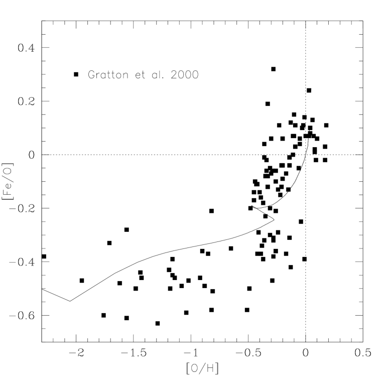
Figure 2a:

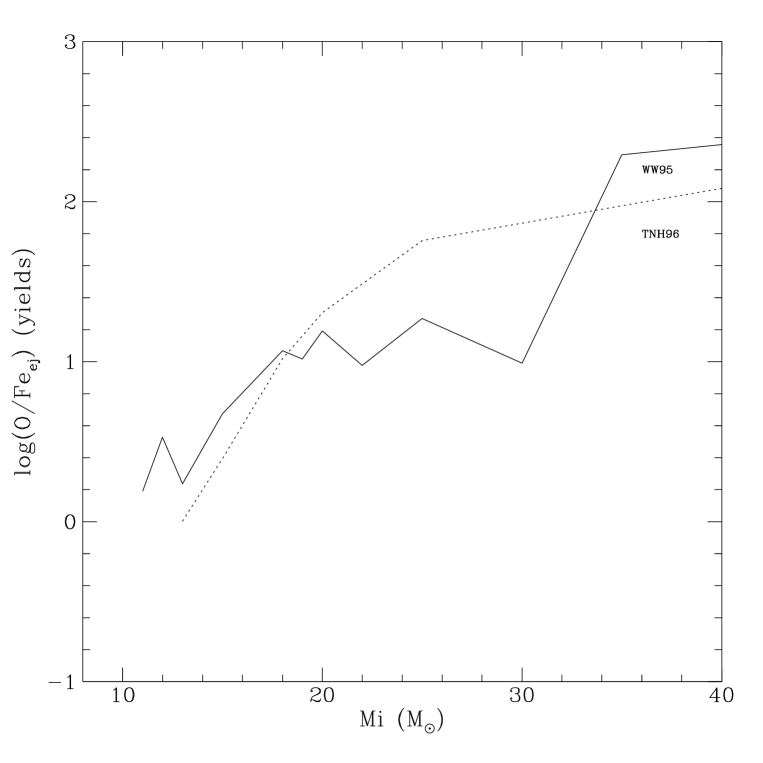
Figure 2b:

Figure 3:

Figure 4:

Figure 5:

Figure 6:

Figure 7:

Figure 8:

Figure 9:

Figure 10:

Figure 11:

Figure 12:

Figure 13:

References

- (1) Afflerbach, A., Churchwell, E., & Werner, M.W. 1997, ApJ, 478, 190
- (2) Allen, C., Carigi, L. & Peimbert, M. 1998, ApJ, 494, 247
- (3) Anders, E., & Grevesse, N. 1989, Geochim. Cosmochim. Acta, 53, 197
- (4) Bahcall, J.N., Flynn, C., & Gould, A. 1992, ApJ, 389, 234
- (5) Beers, T.C., & Sommer-Larsen, J. 1995, ApJS, 96, 175
- (6) Binney, J., Tremaine, S. 1987, Galactic Dynamics (Princeton: Princeton Univ. Press)
- (7) Boesgaard, A. N., King, J. R., Deliyannis, C. P., & Vogt, S. S. 1999, AJ, 117, 492
- (8) Boissier, S., & Prantzos, N. 1999, MNRAS, 307, 857
- (9) Cappellaro, E., & Turatto, M. 1996, in Thermonuclear Supernovae, ed. P. Ruiz-Lapuente, R. Canal, & J. Isern (Kluwer Academic Publishers), 77
- (10) Carigi, L. 1996, Rev. Mex. Astron. & Astrofis., 4, 123
- (11) Carigi, L. 1994, ApJ, 424, 181
- (12) Carraro, G., Ng, Y.K., & Portinari, L. 1998, MNRAS, 296, 1045
- (13) Chang, R.X., Hou, J.L., Shu, C.G., & Fu, C.Q. 1999, A&A, 350, 38
- (14) Chiappini, C., Matteucci, F., & Padoan, P. 2000, ApJ, 528, 711
- (15) Chiappini, C., & Matteucci, F. 2000, in ASP Conf. Ser., the Light Elements and their Evolution, ed. L. da Silva, R. de Medeiros & Spite (San Francisco: ASP), in press
- (16) Chiappini, C., Matteucci, F., Beers, T. & Nomoto, K. 1999, ApJ, 515, 226
- (17) Chiappini, C., Matteucci, F., & Gratton, R. 1997, ApJ, 477, 765 (CMG97)
- (18) Costa, R.D.D., Chiappini, C., Maciel, W.J., & de Freitas Pacheco, J.A. 1997, in Advances in Stellar Evolution (Cambridge: Cambridge Univ. Press), 159
- (19) Crézé, M., Chereul, E., Bienaymé, O., & Pichon, C. 1998, A&A, 329, 920
- (20) Dame, T.M. 1993, in Back to the Galaxy, ed. S. Holt & F. Verter, 267
- (21) Deharveng, L., Peña, M., Caplan, J., & Costero, R. 2000, MNRAS, 311, 329
- (22) Dickey, J.M. 1993, in ASP Conf. Ser. 39, The Minnesota Lectures on the Structure and Dynamics of the Milky Way, ed. R.M. Humphreys (San Francisco: ASP), 93
- (23) Edvardsson, B. 1998, in Abundance Profiles: Diagnostic Tools for Galaxy History, ASP Conference Series, Vol. 147, p.45
- (24) Elmegreen, B.G. 1999, ApJ, 517, 103
- (25) Esteban, C., Peimbert, M., Torres-Peimbert, S., & Escalante, V. 1998, MNRAS, 295, 401
- (26) Esteban, C., Peimbert, M., Torres-Peimbert, S., & García-Rojas, J. 1999a, Rev. Mex. Astron. Astrof., 35, 65
- (27) Esteban, C., Peimbert, M., Torres-Peimbert, S., García-Rojas, J., & Rodríguez, M. 1999b, ApJS, 120, 113
- (28) Ferguson, A., Wyse, R., Gallagher, J.S. 1998 in “Abundance Profiles: Diagnostic Tools for Galaxy History” A.S.P. Conf. Series Vol. 147, p.103
- (29) Fich, M., & Silkey, M. 1991, ApJ, 366, 107
- (30) Fitzsimmons, A., Dufton, P.L., & Rolleston, W.R.J. 1992, MNRAS, 259, 489
- (31) Flynn, C., & Fuchs, B. 1994, MNRAS, 270, 471
- (32) Freudenreich, H. 1998, ApJ, 492, 495
- (33) Friel, E.D., & Janes, K.A. 1993, A&A, 267, 75
- (34) Friel, E.D. 1999, Ap&SS, 265, 271
- (35) Fuhrmann, K. 1998, A&A, 338, 161
- (36) Gehren, T., Nissen, P.E., Kudritzki, R.P., & Butler, K. 1985, in Production and Distribution of CNO Elements, ed. I.J. Danziger, F. Matteucci, & K. Kjaer (Garching: ESO), 171
- (37) Gerritsen, J.P.E., & Icke, V. 1997, A&A, 325, 972
- (38) Gilmore, G., Wyse, R.F.G., & Kuijken, K. 1989, ARA&A, 27, 555
- (39) Gilmore, G., Wyse, R.F.G., & Jones, J.B. 1995, AJ, 109, 1095
- (40) Goswami, A. & Prantzos, N. 2000, A&A, 359, 191
- (41) Gratton, R., Carretta, E., Matteucci, F., & Sneden, C. 1996, in ASP Conf. Ser. 92, Formation of the Galactic Halo — Inside and Out, ed. H. Morrison, & A. Sarajedini (San Francisco: ASP), 307
- (42) Gratton, R.G., Carretta, E., Matteucci, F., & Sneden, C. 2000, A&A, 358, 671
- (43) Grevesse, N., & Sauval, A.J. 1998, Space Sci. Rev., 85, 161
- (44) Guibert, J., Lequeux, J., Viallefond, F. 1978, A&A, 68, 1
- (45) Gummersbach, C.A., Kaufer, A., Schäfer, D.R., Szeifert, T., & Wolf, B. 1998, A&A, 338, 881
- (46) Güsten, R., & Mezger, P.G. 1982, Vistas Astron., 26, 159
- (47) Hensler, G. 1999, Ap&SS, 265, 397
- (48) Holmberg, J., & Flynn, C. 1998, MNRAS, submitted (astro-ph/9812404)
- (49) Hou, J.L., Prantzos, N., & Boissier, S. 2000, A&A, in press
- (50) Hou, J.L., Chang, R. & Fu, C. 1998 in Pacific Rim Conference on Stellar Astrophysics, ASP Conf. Ser, Vol. 138, ed. Kiwing Lam Chan, K.S. Cheng and H.P. Singh, p. 143
- (51) Israelian, G., Garcia-Lopez, R. & Rebolo, R. 1998, ApJ, 507, 805
- (52) Kaufer, A., Szeifert, T., Krenzin, R., Baschek, B., & Wolf, B. 1994, A&A, 289, 740
- (53) Kennicutt, R.C., Jr. 1989, ApJ, 344, 685
- (54) Kennicutt, R.C., Jr. 1998, ApJ, 498, 541
- (55) Kennicutt, R.C., Jr. 2000, in ASP Conf. Ser., Galaxy Disks and Disk Galaxies, (San Francisco: ASP), in press
- (56) Kilian-Montenbruck, J., Gehren, T., & Nissen, P.E. 1994, A&A, 291, 757
- (57) Kobayashi, C., Tsujimoto, T., Nomoto, K., Hachisu, I., Kato, M. 1998, ApJ, 503, 155
- (58) Kuijken, K., & Gilmore, G. 1991, ApJ, 367, L9
- (59) Kulkarni, S.R., & Heiles, C. 1987, in Interstellar processes, ed. D. Hollenbach, & H. Thronson (Kluwer: Dordrecht), 87
- (60) Lacey, C.G., Fall, M. 1985, ApJ, 290, 154
- (61) Larson, R.B. 1976, MNRAS, 176, 31
- (62) Lyne, A.G., Manchester, R.N., Taylor, J.H. 1985, MNRAS, 213, 613
- (63) Maciel, W.J., & Chiappini, C. 1994, Ap&SS, 219, 231
- (64) Maciel, W.J., & Köppen, J. 1994, A&A, 282, 436
- (65) Maciel, W.J. 1997, IAU Symp. 180, ed. H.J. Habing and J. Lamers, Dordrecht, p.397
- (66) Maciel, W.J., & Quireza, C. 1999, A&A, 345, 629
- (67) Maciel, W.J. 2000, in The Chemical Evolution of the Milky Way: Stars versus Clusters, ed. F. Giovannelli, & F. Matteucci (Kluwer: Dordrecht), in press
- (68) Matteucci, F. Greggio, L. 1986, A&A, 154, 279
- (69) Matteucci, F., & François, P. 1989, MNRAS, 239, 885
- (70) Matteucci, F., Ferrini, F., Pardi, C., & Penco, U. 1990, in Chemical and Dynamical Evolution of Galaxies, ed. F. Ferrini, J. Franco & F. Matteucci (Pisa: ETS Editrice), 586
- (71) Matteucci, F. 1991 in Supernova 1987A and Other Supernovae, ESO Workshop, eds. I.J. Danziger and K. Kjär, ESO Publ. p.703
- (72) Matteucci, F. & Chiappini, C. 1999, in Chemical Evolution from zeroto high redshift, ESO Workshop, eds J.R. Walsh and M.R. Rosa, Springer, p.83
- (73) Matteucci, F. 2000, in Euroconference:”The Evolution of Galaxies I- Observational Clues”, ApSS, in press
- (74) Mathews, G. J. & Schramm, D. N 1993, ApJ 404, 468
- (75) Méra, D., Chabrier, G., & Schaeffer, R. 1998, A&A, 330, 937
- (76) Pagel, B.E.J., & Patchett, B.E. 1975, MNRAS, 172, 13
- (77) Pagel, B.E.J., & Tautvaisiene, G. 1995, MNRAS, 276, 505
- (78) Pagel, B.E.J. 2000, in The Chemical Evolution of the Milky Way: Stars versus Clusters, ed. F. Giovannelli, & F. Matteucci (Kluwer: Dordrecht), in press
- (79) Peimbert, M. 1978, in Planetary Nebulae (Kluwer: Dordrecht), 215
- (80) Portinari, L., Chiosi, C., & Bressan, A. 1998, A&A 334, 505
- (81) Portinari, L., & Chiosi, C. 1999, A&A, 350, 827
- (82) Portinari, L., & Chiosi, C. 2000, A&A, 355, 929
- (83) Prantzos, N., & Silk, J. 1998, ApJ, 507, 229
- (84) Prantzos, N., Boissier, S. 2000, MNRAS, 313, 338
- (85) Ramaty, R., Scully, S.T., Lingenfelter, R.E., Lozlovsky, B. 2000, ApJ, 534, 747
- (86) Rana, N.C. 1991, ARA&A, 29, 129
- (87) Reid, M. 1993, ARA&A, 31, 345
- (88) Renzini, A., & Voli, M. 1981, A&A, 94, 175
- (89) Roche, N., Ratnatunga, K., Griffiths, R.E., Im, M., & Naim, A. 1998, MNRAS, 293, 157
- (90) Romano, D. & Matteucci, F. 2000, in The Chemical Evolution of the Milky Way: Stars versus Clusters, ed. F. Matteucci & F. Giovannelli (Kluwer: Dordrecht), p.547
- (91) Romano, D., Matteucci, F., Salucci, P., & Chiappini, C. 2000, ApJ, 539, 235
- (92) Rosenberg, A., Saviane, I., Piotto, G., & Aparicio, A. 1999, AJ, 118, 2306
- (93) Rudolph, A.L., Simpson, J.P., Haas, M.R., Erickson, E.F., & Fich, M. 1997, ApJ, 489, 94
- (94) Sackett, P.D. 1997, ApJ, 483, 103
- (95) Samland, M., Hensler, G., & Theis, C. 1997, ApJ, 476, 544
- (96) Scalo, J.M. 1986, Fundam. Cosmic Phys., 11, 1
- (97) Searle, L., Zinn, R. 1978 ApJ, 225, 357
- (98) Shafter, A.W. 1997, ApJ, 487, 226
- (99) Shaver, P.A., McGee, R.X., Newton, L.M., Danks, A.C., & Pottasch, S.R. 1983, MNRAS, 204, 53
- (100) Simard, L., Koo, D.C., Faber, S.M., Sarajedini, V.L., Vogt, N.P., Phillips, A.C., Gebhardt, K., Illingworth, G.D., & Wu, K.L. 1999, ApJ, 519, 563
- (101) Simpson, J.P., Colgan, S.W.J., Rubin, R.H., Erickson, E.F., & Haas, M.R. 1995, ApJ, 444, 721
- (102) Smartt, S.J., & Rolleston, W.R.J. 1997, ApJ, 481, L47
- (103) Thielemann, F. K., Nomoto, K., Hashimoto, M. 1996, ApJ 460, 408
- (104) Timmes, F. X., Woosley, S.E., & Weaver, T. A. 1995, ApJS, 98, 617
- (105) Tosi, M. 1988, A& A, 197, 47
- (106) Tosi, M. 1996, in ASP Conf. Ser. 98, From Stars to Galaxies: The Impact of Stellar Physics on Galaxy Evolution, ed. C. Leitherer, U. Fritze-von-Alvensleben, & J. Huchra (San Francisco: ASP), 299
- (107) Tosi, M. 2000, in The Chemical Evolution of the Milky Way: Stars versus Clusters, ed. F. Giovannelli, & F. Matteucci (Kluwer: Dordrecht), in press
- (108) Tsujimoto, T., Yoshii, Y., Nomoto, K., Shigeyama, T. 1995 A&A, 302, 704
- (109) Twarog, B.A., Ashman, K.M., & Anthony-Twarog, B.J. 1997, ApJ, 114, 2556
- (110) van den Hoek, L.B., & Groenewegen, M.A.T. 1997, A&AS, 123, 305
- (111) van der Hulst, J.M., Skillman, E.D., Smith, T.R., Bothum, G.D., McGaugh, S.S. & de Blok 1993, AJ, 106, 548
- (112) Viegas, S.M., Gruenwald, R., & Steigman, G. 2000, ApJ, 531, 813
- (113) Vílchez, J.M., & Esteban, C. 1996, MNRAS, 280, 720