Ultraviolet and Visible Spectropolarimetric Variability in P Cygni
Abstract
We report on new data, including four vacuum ultraviolet spectropolarimetric observations by the Wisconsin Ultraviolet Photo-Polarimeter Experiment (”WUPPE”) on the Astro-1 and Astro-2 shuttle missions, and 15 new visible-wavelength observations obtained by the HPOL CCD spectropolarimeter at the Pine Bluff Observatory of the University of Wisconsin. This includes three HPOL observations made within 12 hours of each of the three Astro-2 WUPPE observations, giving essentially simultaneous observations extending from to . An analysis of these data yields estimates on the properties of wind ”clumps” when they are detectable by the polarization of their scattered light. We find that the clumps must be detected near the base of the wind, . At this time the clump density is at least , 20 times the mean wind, and the temperature is roughly 10,000 ∘K, about cooler than the mean wind. The clumps leading to the largest observed polarization must have electron optical depth of 0.1 - 1 and an angular extent of 0.1 - 1 ster, and account for at most of the wind mass loss. The H and HeI emission lines from the wind are unpolarized, but their P Cygni absorption is enhanced by a factor of four in the scattered light. We speculate on the possible relationship of the clumps detected polarimetrically to those seen as Discrete Absorption Components (DACs) and in interferometry.
Space Astronomy Lab, University of Wisconsin, Madison WI 53706
Space Telescope Science Institute, Baltimore MD 21218
1. Introduction
P Cygni was found by many early polarimetric investigators to possess intrinsic linear polarization (eg, Coyne & Gehrels 1967; Coyne, Gehrels, & Serkowski 1974; Serkowski, Mathewson, & Ford 1975). Hayes (1985) and Lupie & Nordsieck (1987) established that the polarization was variable on timescales of days - weeks, with an amplitude of approximately 0.4%, and with no apparent periodicity nor favored position angle, although the interpretation was hampered by an appreciable, unknown interstellar polarization. The long time series of Hayes (1985) exhibits a polarimetric episode length of week, and a repetition rate of once per 20-30 days. Taylor, Nordsieck et al (1991, hereafter ”TN”), in the first detailed spectropolarimetric investigation, made use of the apparent non-variability of the polarization of the emission line to estimate the interstellar polarization there, extrapolating to other wavelengths using a galactic mean interstellar wavelength dependence. After removing this interstellar polarization, TN then confirmed the remarkable daily variability and the random nature of the degree and position angle of the intrinsic continuum polarization. The , , and lines were found to be essentially unpolarized, while the continuum polarization wavelength dependence is not flat, but exhibits a steady decrease from the near ultraviolet into the red. TN pointed out that this, coupled with the lack of a polarization Balmer Jump, was difficult to explain using the model which is conventionally used for Be stars, where hydrogen bound-free opacity competes with wavelength-independent electron scattering to impart a polarization wavelength dependence.
2. New Spectropolarimetry
The new polarimetric data presented here includes four vacuum ultraviolet spectropolarimetric observations by WUPPE on the shuttle missions Astro-1 (one observation: 12 Dec, 1990) and Astro-2 (three observations: 3, 8, and 12 March, 1995), and 15 new visible-wavelength observations obtained by the ”HPOL” CCD spectropolarimeter at the Pine Bluff Observatory of the University of Wisconsin. The WUPPE instrument is described in Nordsieck et al (1994) and HPOL is described in Nordsieck & Harris (1995). The visible wavelength spectropolarimetry includes three HPOL observations made within 12 hours of each of the three Astro-2 WUPPE observations, giving essentially simultaneous observations extending from to . The Astro-1 WUPPE observation was discussed by Taylor, Code, et al (1991), who noted a total continuum polarization generally consistent with interstellar, plus possible line-blanketing of the intrinsic polarization, an effect similar to that observed in WUPPE observations of Be stars (Bjorkman, et al 1991).
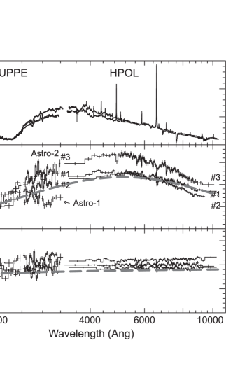
Figure 1 shows the net polarization vs wavelength from the WUPPE observations and the three contemporaneous HPOL observations. The observations exhibit an overall interstellar polarization continuum shape plus strong intrinsic polarization variability over most of the spectrum. The interstellar polarization is estimated in a variety of ways. First, we see that the four WUPPE observations all cross in the region. We interpret this to be strong FeIII line blanketing which is suppressing the intrinsic polarization there. This region is known to be the most strongly blanketed region in P Cyg (Pauldrach and Puls 1990), and strong polarization suppression there is seen similarly in the Be star Tau (Bjorkman, et al 1991). Conveniently, this then establishes the interstellar polarization value at , at PA 32.1. Second, following TN, the line is assumed to be not intrinsically polarized.
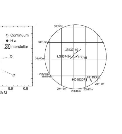
This is supported by figure 2a, which shows a polarization vector diagram for all of the HPOL observations. The continuum polarization near varies by roughly with no apparent favored position angle, while the points are consistent with a constant polarization of at PA 35.5. This is then taken to be the interstellar polarization at (cross in figure 2a). Using the standard Serkowski interstellar polarization law as modified by Wilking, Lebowski, & Rieke (1987; ”WLR”), plus a modest position angle rotation, these two points determine the actual P Cyg WLR parameters: , , , and a position angle rotation of . The adopted interstellar polarization curve is shown as the gray dashed line in figure 1. We have attempted to verify the above estimate through observations of stars near P Cyg (figure 2b). Observations with HPOL with the 0.9m telescope at PBO of HD19300 and HD19307 (17 arcmin distant) exhibit rather different interstellar polarizations, consistent with the large known variations in Cygnus. New observations at the WIYN 3.5m telescope of two B stars less than 5 arcmin distant within the P Cyg cluster, LSII 37-49 and -54, yield more comparable results, 1.5% at and 0.9% at . This provides support for our adopted value.
3. Intrinsic Polarization
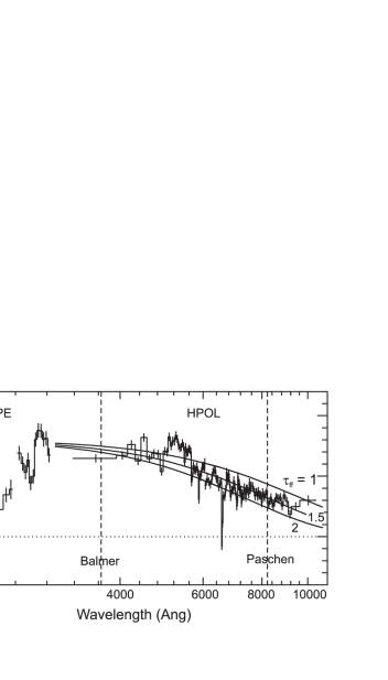
In Figure 3 we show the mean intrinsic polarization wavelength dependence for the three Astro-2 + HPOL observations. This was obtained by removing the fitted interstellar polarization, rotating the intrinsic polarization into the Q stokes parameter using the blue position angle, and averaging the result. This is the same procedure used by TN to estimate the mean wavelength dependence of the intrinsic polarization: it assumes that the intrinsic polarization at one time has a position angle independent of wavelength. The Stokes polarization Q is positive when the polarization is parallel to the blue continuum polarization, and negative when it is orthogonal. Note the strong decrease into the vacuum ultraviolet (presumably due to line blanketing), the strong decrease into the red as noted by TN but here extended into the near infrared, and the lack of both a Balmer and Paschen jump .
3.1. Clump Optical Depth
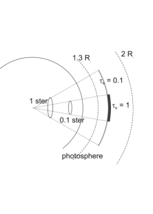
It is assumed that for a star as hot as P Cyg, any continuum intrinsic polarization is due to electron scattering in the envelope, presumably in asymmetric inhomogeneities (”clumps”). We may estimate the electron scattering optical depth of the clumps from a simple single-scattering analysis of the degree of polarization. Using formulae in Cassinelli, Nordsieck, and Murison (1987), the net polarization from a sector- shaped density enhancement subtending ster and with electron scattering optical depth is
Here is the inclination of the clump direction to the line of sight, and is the ”finite disk correction factor” which corrects for cancellation of polarization near the stellar photosphere caused by illumination from a non-point source (here we take the approximation of no photospheric limb darkening). Given the rapid timescale and the large amount of polarization observed, we expect that the clumps are polarimetrically observable only near the base of the wind. Later we find that the appropriate value for the radial position of the clumps is , which gives for (Najarro 2000); we will take . This formula holds approximately until , where the clump becomes optically thick to the total opacity, and ster, where geometric cancellation over the clump begins to reduce the polarization. Thus the maximum possible polarization (for ) is
The observed polarization amplitude below is roughly 0.004, so that . A range of clump properties consistent with the observations is then to .
3.2. Free-Free Absorption - Clump Density
The presence of continuum absorption optical depth in addition to the electron scattering optical depth reduces the net polarization by the absorption in the clump
where is the total flux and is the polarized scattered flux. Features in may then be used to estimate , and thus the physical properties of the clumps.
An important feature of the observed continuum intrinsic polarization wavelength dependence is the persistent decrease into the infrared. This was also noted by TN, and holds for individual nights as well as the mean. A plausible explanation for this, given the high density and ionization at the base of the wind, is competing free-free absorptive opacity. Since , the polarization will decrease into the red as . Figure 3 shows a fit to the polarization for , , and . We adopt as the best value. Given our the range of allowed , we have . This provides an estimate of the clump electron density:
(For these rough estimates we assume a highly ionized pure hydrogen gas, is the clump temperature in units of , and is the Gaunt factor). This is approximately 20 times the density in the wind at these radii in the model of Najarro (2000).
3.3. Bound-Free Jumps: Clump Temperature and Ionization
The lack of Balmer or Paschen Jumps in the intrinsic polarization of figure 3 puts an upper limit for neutral hydrogen bound-free absorption in the clumps, which then means . This ultimately puts a limit on the clump temperature:
where is the neutral fraction and is the departure coefficient for the second state of hydrogen in the clump. For simplicity we will assume that is unchanged in the clump; it is less than two at the base of the wind in the models of Najarro (2000), in any case. For , we assume pure optically thin photoionization, so that it may be scaled from the base wind density and temperature:
Finally, then,
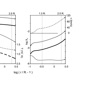
Given a wind model, this may be solved for , giving the maximum temperature of the clump consistent with no detectable bound-free absorption. Notice that this is independent of clump electron scattering optical depth and density. Figure 4 (heavy lines) shows the clump density and ionization corresponding to the maximum temperature at each radius in the wind, using the wind model of Najarro (2000), for and . The clumps will not be detectable inside , the position of the photosphere. Above , the maximum temperature decreases below and recombination must occur; this puts a rough upper limit on the radius.
The clumps must contribute their maximum polarization from to , and at this time they must be at least 20 times more dense and 20% cooler than the wind.
3.4. Clump Geometry and Time Evolution
It is interesting to compare the geometric properties of the range of possible clumps. ”Thin” clumps have and . ”Thick” ones have and . The physical thickness of these clumps is and , respectively, at . Figure 5 illustrates this ”pancake-like” geometry. The mass of the thick and thin clumps is the same, a result of the requirement that they produce the same polarization. The instantaneous stellar mass loss rate due to a clump compared to that in the base wind is and at , which lasts for a time and day, respectively. Given that the repetition rate for polarimetric clumps is 20 - 30 days, these clumps account for at most 1% of the mass loss of the star. The largest mass clumps are required at the largest distance from the star: at , they still account for at most 2% of the wind mass loss.
Finally, we may speculate on the time evolution of the clumps and their polarization. This will depend on the evolution of the mass and density of the clumps as they are carried out in the wind. The analysis above has placed limits on the properties of the clumps at the time that they contribute the largest polarization. The polarization will grow as the clump appears out of the photosphere, possibly growing in mass as it forms. It may then dissipate and its density, optical depth, and polarization will drop as it is carried out in the wind. This is a complex problem requiring a proper radiative transfer and clump physics model. We may explore the purely geometric effects, however: if we ignore optical depth effects and changes in clump mass, . This has a maximum at , and drops by a factor of 10 by . This is consistent with the polarizing clumps being highly ionized: by the time they reach the recombined part of the wind, the polarization is no longer detectable. The time it takes for a clump to traverse the region will be days, which compares favorably with the observed duration of roughly one week.
3.5. Intrinsic Line Polarization
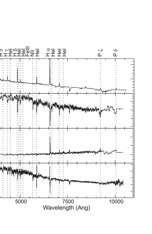
Figure 6 shows an expanded version of the visible-wavelength mean intrinsic polarization spectrum from all 15 HPOL observations. The improved sensitivity of the new HPOL data allows one to extend the TN analysis to 4 Hydrogen lines and 5 HeI lines. The intrinsic polarization of the emission line flux itself is a diagnostic of the wind. Any line radiation produced deep in the wind may become polarized if it is scattered off the clumps that produce the continuum polarization. Alternatively, the P-Cygni absorption beneath the emission line (unresolved in these observations) may be different in the clump, producing an apparent line polarization. The latter appears to be the largest effect in P Cyg.
The line Stokes polarization is conventionally computed as follows:
where the integral is performed over the observed line profile, and and are the flux and Stokes polarization in the neighboring continuum. The initially surprising result is that the weaker lines all appear to be negatively polarized (polarized orthogonal to the continuum). We believe that this is an artifact of the fact that the P Cygni absorption is enhanced in the clumps, and is as a result interpreted as emission polarized orthogonal to the continuum. For such a situation one can show that the apparent net Stokes polarization of the line is
where and are the Stokes polarization of the emission line and continuum, respectively, and are the equivalent widths of the absorption and emission part of the P-Cygni line, respectively, and is the factor by which the absorption line is enhanced in the polarized light. and were evaluated using the mean P Cyg line profiles in Stahl, et al (1993).
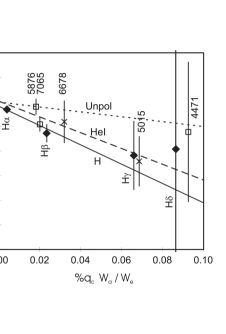
In Figure 7 we plot versus for the 9 lines measured. In this plot, the intercept of a straight line fit to the lines of one species is and the slope is . The line labeled ”unpol” in this diagram corresponds to and . We see that both the H and HeI lines are consistent with unpolarized emission (), implying that more than of the emission arises outside of the polarizing region. On the other hand, both H and HeI are strongly enhanced in absorption in the polarized flux (). The enhancement must be due to a complex combination of ionization and excitation effects, and will require a detailed analysis. It is perhaps surprising that the values are so similar for H and HeI. Another way of seeing these effects is in the bottom panel of figure 6, the ”polarized flux”. This is essentially the spectrum of the scattered light: the emission lines have almost vanished, indicating the emission is unscattered, and strong absorption is seen instead.
4. Relation of Polarimetry to other Observations
A frequently mentioned datum for P Cyg is the apparent rotation from measurements. Markova (2000) favors a value of 40 km/s, and it is agreed that values less than 25 km/sec are not consistent with absorption line depths. 40 km/s is of breakup velocity for a , star (270 km/s). This is large enough that one might expect a substantially flattened wind if viewed edge-on. However, the intrinsic polarization does not show a favored position angle: In figure 2a the continuum polarization points occupy a nearly circular region. By contrast, Be stars, which are rotating at break-up, show polarization vector diagrams confined to a narrow line. One way out of this apparent contradiction is if P Cyg is rotating rapidly, and is viewed not quite pole-on. For such an object, assuming that all clumps are ejected at random in the equatorial plane, the expected axial ratio in the polarization vector diagram is . If we insist that , this gives . This in turn gives km/s, which is still breakup. This would likely be a bipolar object, but viewed nearly pole-on. Several things recommend this scenario: First, P Cyg has an unusually high wind speed among S Dor variables (Luminous Blue Variables). This would be explained if we are just observing a fast polar wind in a bipolar object. Second, most S Dor’s are bipolar. And third, most clumps would be ejected near the plane of the sky, which is favorable for large polarimetric variations. On the other hand, spectroscopy of the P Cyg shell (Meaburn 2000) does not show the characteristic multiple- redshift components seen in bipolar Planetary Nebulae, for instance. The pole-on hypothesis is testable by looking for a systematic daily change in the polarimetric position angle. During the 14 days of detectability, a clump would rotate about 60∘about the star, and each successive clump would exhibit the same sense of rotation.
How might the polarimetric clumps be related to the Discrete Absorption Components (DAC’s) seen in P Cyg? If there were no rotation, or the object is viewed pole-on, they would probably be uncorrelated, since polarimetric clumps must be ejected near the plane of the sky and would never cover the stellar disk to form DAC’s. On the other hand, if the star is seen equator-on and is rotating at km/s, a clump will have rotated about 20∘by the time it reaches , and by (if the clump maintains its integrity this long). This suggests that there would be a weeks - month time delay between the appearance of a polarimetric clump and its observability as a DAC. This correlation would vary with the initial ejection longitude of the clump. Given the relatively frequent generation of polarimetric clumps (20-30 days), such a variable delay might be difficult to establish.
On the other hand, the polarimetric clumps should certainly be related to clumps observed interferometrically (Chesneau, et al 2000). If the clump does not disintegrate first, there should be a roughly 2-6 week delay between the appearance of a polarimetric clump and its detectability as an clump at . The position angles of the polarimetric and interferometric clumps should be correlated, and systematic differences in position angle would be a sensitive measure of the component of stellar rotation about the line of sight (which combined with would yield the inclination).
5. Summary; Future
In summary, we have analyzed the variability of the wavelength dependence of the polarization of P Cyg from . After removal of the interstellar polarization, we have put limits on the properties of the wind inhomogeneities (”clumps”) during the brief period that they are detectable in polarization.
-
•
The presence of free-free absorption in the polarization wavelength dependence implies a clump electron density of at least . This corresponds to a density contrast of at least 20 at the base of the wind.
-
•
The absence of Balmer and Paschen bound-free absorption in the polarization limits the polarimetric zone to , where the hydrogen ionization is high, and requires the clumps to be substantially cooler than the wind. The clumps take 14 days to be swept through this region.
-
•
In order to produce the maximum observed polarization, the largest clumps must have an electron optical depth of 0.1 - 1 and an angular extent of 0.1 - 1 ster, accounting for at most of mean mass loss of the wind.
-
•
The emission lines are essentially unpolarized. However, the P Cygni absorption is enhanced by a factor of four in the polarimetric clumps.
We plan on the following further observational investigations:
-
•
Higher spectral resolution spectropolarimetry to resolve polarimetric line profiles. This should verify the line analysis model of section 3.5.
-
•
Monitor the polarization every night for at least a month. During such a campaign we would look for a change in polarization wavelength dependence during an episode, including the expected decease in the free-free absorption and the possible appearance of bound-free jumps near the beginning or end of the episode. We would also look for a systematic position angle change with time, indicating rotation. We will attempt to arrange simultaneous high-resolution spectroscopy (for DACs) and interferometry, to pursue the predictions of section 4.
For modeling, we plan to develop our Monte Carlo polarization radiation transfer code to give a quantitative continuum polarization model based on the mean wind from Najarro (2000), including electron scattering, H bound free, H free-free, and line blanketing, with a simple sector geometry. This would predict the absolute degree of polarization, the continuum wavelength dependence, and their time dependence as the clump is carried out in the wind. Variables would include the clump heating/ cooling and confinement mechanisms.
A more ambitious polarization model would treat the lines. To accomplish this, it will be necessary to more correctly model the ionization and populations in the clump. Such a model would predict equivalent width in polarized flux for H and HeI to compare with the observations. Finally, our ultimate goal is to calculate polarimetric line profiles, allowing for electron scattering broadening and Doppler shifts in the wind, to compare with future high resolution observations.
Acknowledgments.
WUPPE was supported by NASA contract NAS5-26777. The analysis reported in this paper is supported by a NASA Astrophysics Data Program grant, NAG5-7931. We gratefully acknowledge Francisco Najarro for sending early results from his P Cyg wind model, and very useful discussions with Henny Lamers, Joe Cassinelli, and John Mathis.
References
Bjorkman, K.S., Nordsieck, K.H., Code, A.D. et al 1991 ApJ, 383, L67
Cassinelli, J.P., Nordsieck, K.H., & Murison, M. 1987, ApJ., 317, 290
Chesneau, O., Vakili, F., Abe, L., Roche, M., Aime, C., & Lanteri H. 2000 This Conference
Coyne, G.V. & Gehrels, T. 1967 AJ, 72, 887
Coyne, G.V.,Gehrels, T., & Serkowski, K. 1974 AJ, 79, 581
Hayes, D.P 1985 ApJ, 289, 726
Lupie, O.L. & Nordsieck, K.H. 1987 AJ, 92, 214
Meaburn, J. 2000. This Conference
Markova, N. 2000. This Conference
Najarro, F. 2000. This Conference
Nordsieck, K.H. & Harris, W. 1995 in Polarimetry of the Interstellar Medium (ed. W.G. Roberge and D.C.B. Whittet) ASP Conf Ser 97: San Francisco
Nordsieck, K.H., Marcum, P., Jaehnig, K.P., and Michalski, D.E. 1994. Proc SPIE 2010, p 28
Pauldrach, A.W.A. & Puls, J. 1990 A&A, 237, 409
Serkowski, K. Mathewson, D.S., & Ford, V.L. 1975 ApJ, 196, 261
Stahl, O., Mandel, H., Wolf, B., G ng, Th., Kaufer, A., Kneer, R., Szeifert, Th., & Zhao, F. 1993 A&AS, 99, 167
Taylor, M., Code, A.D., Nordsieck, K.H., et al 1991 ApJ, 382, L85
Taylor, M., Nordsieck, K.H., Schulte-Ladbeck, R.E., & Bjorkman, K.S. 1991 (”TN”) AJ, 102, 1197
Wilking, B.A., Lebofsky, M.J., & Rieke, G.H. 1982, AJ, 87, 695