[From Clustering to Homogeneity]Clustering in the Universe: from Highly Nonlinear Structures to HomogeneityL Guzzo
Osservatorio Astronomico di Brera

1 Introduction

This chapter concentrates on a few specific topics concerning the distribution of galaxies on scales from 0.1 to nearly 1000 $h^{-1}\,{\rm Mpc}\;$. The main aim is to provide the reader with the information and tools to familiarize with a few basic questions: 1) What are the scaling laws followed by the clustering of luminous objects over almost four decades of scales; 2) How galaxy motions distort the observed maps in redshift space, and how we can correct and use them to our benefit; 3) Is the observed clustering of galaxies suggestive of a fractal Universe; and consequently, 4) Is our faith in the Cosmological Principle still well placed, i.e. do we see evidence for a homogeneous distribution of matter on the largest explorable scales, in terms of the correlation function and power spectrum of the distribution of luminous objects. For some of these questions we have a well–defined answer, but for some others the idea is to indicate the path along which there is still a good deal of exciting work to be done.

2 The clustering of galaxies

I believe most of the students attending this School are familiar with the beautiful cone diagrams showing the distribution of galaxies in what have been often called slices of the Universe. This has been made possible by the tremendous progress in the efficiency of redshift surveys, i.e. observational campaigns aimed at measuring the distance of large samples of galaxies through the cosmological redshift observed in their spectra. This is one of the very simple, yet fundamental pillars of observational cosmology: reconstructing the three–dimensional positions of galaxies in space to be able to study and characterise statistically their distribution. Figure 1 shows the current status of the ongoing 2dF survey and gives an idea of the state of the art, with $\sim 130,000$ redshifts measured and a planned final number of 250,000 [1]. From this plot, the main features of the galaxy distribution can be appreciated. One can easily recognize clusters, superclusters and voids, and get the feeling on how the galaxy distribution is extremely inhomogeneous to at least 50 $h^{-1}\,{\rm Mpc}\;$(see [2] for a more comprehensive review).

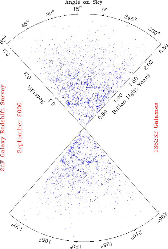
Figure 1: The distribution of the nearly 140,000 galaxies observed so far (September 2000) in the 2dF survey (from [3]): compare this picture to that in [2] to see how rapidly this survey is progressing towards its goal of 250,000 redshifts measured (note that this is a projection over a variable depth in declination, due to the survey being still incomplete).

The inhomogeneity we clearly see in the galaxy distribution can be quantified at the simplest level by asking what is the excess probability over random to find a galaxy at a separation $r$ from another one. This is one way by which one can define the two–point correlation function, certainly the most perused statistical estimator in Cosmology (see [5] for a more detailed introduction). When we have a catalogue with only galaxy positions on the sky (and usually their magnitudes), however, the first quantity we can compute is the angular correlation function $w(\theta)$. This is a projection of the spatial correlation function $\xi(r)$ along the redshift path covered by the sample. The relation between the angular and spatial functions is expressed for small angles by the Limber equation (see [4] and [5] for definitions and details)

$$w(\theta)=\int_{0}^{\infty}dv\,v^{4}\,\phi^{2}(v)\int_{-\infty}^{\infty}du\,\xi\left(\sqrt{u^{2}+v^{2}\theta^{2}}\right)\,\,\,\,\,,$$ (1)

where $\phi(v)$ is the radial selection function of the two–dimensional catalogue, that in this version gives the comoving density of objects at a given distance $v$ (which depends, for example, on the magnitude limit of the catalogue and the specific luminosity function of the type of galaxies one is studying). For optically–selected galaxies [6, 7] $w(\theta)$ is well described by a power–law shape $\propto\theta^{-0.8}$, corresponding to a spatial correlation function $(r/r_{o})^{\gamma}$, with $r_{o}\simeq 5\,h^{-1}\,{\rm Mpc}\;$ and $\gamma\simeq-1.8$, and a break with a rapid decline to zero around scales corresponding to $r\sim 30\,h^{-1}\,{\rm Mpc}\;$.

The advantage of angular catalogues still at present is the large number of galaxies they include, up to a few millions [6]. Since the beginning of the eighties (e.g. [8]), redshift surveys allowed us to compute directly $\xi(r)$ in three–dimensional space, and the most recent samples have pushed these estimates to separations of $\sim 100$ $h^{-1}\,{\rm Mpc}\;$(e.g. [9]). Figure 2 shows the two–point correlation function in redshift space, indicated as $\xi(s)$, for a representative set of published redshift surveys [9, 10, 11, 12]. In addition, the dotted lines show the real–space $\xi(r)$ obtained through de–projection of the angular $w(\theta)$ from the APM galaxy catalogue [13]. The two different lines correspond to two different assumptions about galaxy clustering evolution, which has to be taken into account in the de–projection, given the depth of the APM survey. This illustrates some of the uncertainties inherent in the use of the angular function.

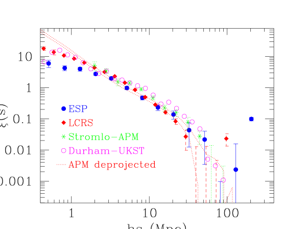
Figure 2: The two–point correlation function of galaxies, as measured from a few representative optically–selected surveys (from [2]). The plot shows results from the ESP [9], LCRS [10], APM-Stromlo, [11] and Durham-UKST [12] surveys, plus the real–space $\xi(r)$ de–projected from the angular correlation function $w(\theta)$ of the APM survey [13].

As can be seen from the Figure, the shape of $\xi(s)$ below $5-10\,h^{-1}\,{\rm Mpc}\;$ is reasonably well described by a power law, but for the four redshift samples the slope is shallower than the canonical $\sim-1.8$ nicely followed by the APM $\xi(r)$. This is due to the redshift–space smearing of structures that suppresses the true clustering power on small scales, as we shall discuss in the following section. Note how $\xi(s)$ maintains a low–amplitude, positive value out to separations of more than $50\,h^{-1}\,{\rm Mpc}\;$, showing explicitly why large–size galaxy surveys are important: we need large volumes and good statistics to be able to extract such a weak clustering signal from the noise. Finally, the careful reader might have noticed a small but significant positive change in the slope of the APM $\xi(r)$ (the only one for which we can see the undistorted real–space clustering at small separations), around $r\sim 3-4\,h^{-1}\,{\rm Mpc}\;$. On scales larger than this, all data show a “shoulder” before breaking down. This inflection point appears around the scales where $\xi\sim 1$, thus suggesting a relationship with the transition from the linear regime (where each mode of the power spectrum grows by the same amount and the shape is preserved), to fully nonlinear clustering on smaller scales [14]. We shall come back to this in §4.

3 Our distorted view of the galaxy distribution

We just had an explicit example of how unveiling the true scaling laws describing galaxy clustering from redshift surveys is complicated by the effects of galaxy peculiar velocities. Separations between galaxies – indicated as $s$ to remark this very point – are not measured in real 3D space, but in redshift space: what we actually measure when we take the redshift of a galaxy is the quantity $cz=cz_{\rm true}+v_{\rm pec//}$, where $v_{\rm pec//}$ is the component of the galaxy peculiar velocity along the line of sight. This quantity, while being typically $\sim 100\,{\rm km\,s^{-1}}$ for “field” galaxies, can rise above $1000\,{\rm km\,s^{-1}}$ in rich clusters of galaxies. As explicitly visible in Figure 2, the resulting $\xi(s)$ is flatter than its real–space counterpart. This is the result of two concurrent effects: on small scales, clustering is suppressed by high velocities in clusters of galaxies, that spread close pairs along the line of sight producing in redshift maps what are sometimes called “Fingers of God”. Many of these are recognisable in Figure 1 as thin radial structures, particularly in the denser part of the upper cone. The net effect on $\xi(s)$ is in fact to suppress its amplitude below $\sim 1-2\,h^{-1}\,{\rm Mpc}\;$. On the other hand, on larger scales where motions are still coherent, streaming flows towards higher–density structures enhance their apparent contrast when they appear to lie perpendicularly to the line of sight. This, on the contrary, amplifies $\xi(s)$ above $10-20\,h^{-1}\,{\rm Mpc}\;$. Both effects can be better appreciated with the help of a computer N–body simulation, for which we have the leisure to see both a real– and a redshift–space snapshot, as in Figure 3.

Figure 3: Particle distribution from a 1–degree thick mock survey through a large–size Tilted–CDM n-body simulation in real (top) and redshift space (bottom). The appearance of the two diagrams gives a clear visual impression of the effect of redshift–space distortions (note that here, unlike in the real survey of Figure 1, no apparent luminosity selection is applied, i.e. the sample is volume limited).

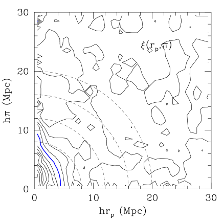
Figure 4: The typical appearance of the bidimensional correlation function $\xi(r_{p},\pi)$, in this specific case computed for the ESP survey [9]. Note the elongation of the contours along the $\pi$ direction for small values of $r_{p}$, produced by high–velocity pairs in clusters. The dashed circles show contours of equal correlation in the absence of distortions.

How could we recover the correlation function of the undistorted spatial pattern, i.e. $\xi(r)$? This can be accomplished by computing the two–dimensional correlation function $\xi(r_{p},\pi)$, where the radial separation $s$ of a galaxy pair is split into two components, $\pi$, parallel to the line of sight, and $r_{p}$, perpendicular to it, defined as follows [15]. If ${\bf d}_{1}$ and ${\bf d}_{2}$ are the distances to the two objects (properly computed) and we define the line of sight vector ${\bf l}\equiv({\bf d}_{1}+{\bf d}_{2})/2$ and the redshift difference vector ${\bf s}\equiv{\bf d}_{1}-{\bf d}_{2}$, then one defines

$$\pi\equiv{{{\bf s}\cdot{\bf l}}\over{|{\bf l}|}}\quad\quad r_{p}^{2}\equiv{{\bf s}\cdot{\bf s}}-\pi^{2}\,\,\,.$$ (2)

The resulting correlation function is a bidimensional map, whose contours at constant correlation look as in the example of Figure 4. By projecting $\xi(r_{p},\pi)$ along the $\pi$ direction, we obtain a function that is independent of the distortion,

$$w_{p}(r_{p})\equiv 2\int_{0}^{\infty}d\pi\,\xi(r_{p},\pi)=2\int_{0}^{\infty}dy\,\xi_{R}\left[(r_{p}^{2}+y^{2})^{1/2}\right]\,,$$ (3)

and is directly related to the real–space correlation function (here indicated with $\xi_{R}(r)$ for clarity), as shown. Modelling $\xi_{R}(r)$ as a power law, $\xi_{R}(r)=(r/r_{0})^{-\gamma}$ we can carry out the integral analytically, yielding

$$w_{p}(r_{p})=r_{p}\left({r_{0}\over r_{p}}\right)^{\gamma}{\Gamma({1\over 2})\,\Gamma({\gamma-1\over 2})\over\Gamma({\gamma\over 2})}$$ (4)

where $\Gamma$ is the Gamma function. Such form can then be fitted to the observed $w_{p}(r_{p})$ to recover the parameters describing $\xi(r)$ (e.g. [16]). Alternatively, one can perform a formal Abel inversion of $w_{p}(r_{p})$ [17].

So far, we have treated redshift–space distortions nearly as only an annoying feature that prevents the true distribution of galaxies to be directly seen. In fact, being a dynamical effect they carry precious direct information on the distribution of mass, independently from the distribution of luminous matter. This information can be extracted, in particular by measuring the value of the pairwise velocity dispersion $\sigma_{12}(r)$. This is in practice a measure of the small–scale “temperature” of the galaxy soup, i.e. the amount of kinetic energy produced by the differences in the potential energy created by density fluctuations. Thus, finally, a measure of the mass variance on small scales.

$\xi(r_{p},\pi)$ can be modelled as the convolution of the real–space correlation function with the distribution function of pairwise velocities along the line of sight [8, 18], Let $F({\bf w},r)$ be the distribution function of the vectorial velocity differences ${\bf w}={\bf u}_{2}\ -{\bf u}_{1}\$ for pairs of galaxies separated by a distance $r$ (so a function of four variables, $w_{1}$, $w_{2}$, $w_{3}$, $r$). Let $w_{3}$ be the component of w along the direction of the line of sight (that defined by ${\bf l}$); we can then consider the corresponding distribution function of $w_{3}$,

$$f(w_{3},r)=\int dw_{1}\,dw_{2}\,F({\bf w},r)\,\,\,\,,$$ (5)

It is this distribution function that is convolved with $\xi(r)$ to produce the observed $\xi(r_{p},\pi)$. If we now call $y$ the component of the separation $r$ along the line of sight, with our convention we have that $w_{3}=H_{o}(\pi-y)$ and the convolution

$$1+\xi(r_{p},\pi)=\left[1+\xi(r)\right]\otimes f(w_{3},r)\,\,\,\,,$$ (6)

can be expressed as

$$1+\xi(r_{p},\pi)=H_{\circ}\int_{-\infty}^{+\infty}dy\left\{1+\xi\left[(r_{p}^{2}+y^{2})^{1\over 2}\right]\right\}\,f\left[H_{\circ}(\pi-y)\right]\,\,\,.$$ (7)

Note that this expression gives essentially a model description of the effect produced by peculiar motions on the observed correlations, but does not take into account the intimate relation between the mass density distribution and the velocity field which is in fact a product of mass correlations (see [19] and [20] and references therein). Within this model, therefore, we have no specific physical reason for choosing one or another form for the distribution function $f$. Peebles [21] first showed that an exponential distribution best fits the observed data, a result subsequently confirmed by N–body models [22]. According to this choice, $f$ can then be parameterised as

$$f(w_{3},r)={1\over\sqrt{2}\sigma_{12}(r)}\exp\left[{-\sqrt{2}\left|{w_{3}(r)-\langle w_{3}(r)\rangle\over\sigma_{12}(r)}\right|}\right]\,\,\,,$$ (8)

where $\langle w_{3}(r)\rangle$ and $\sigma_{12}(r)$ are respectively the first and second moment of $f$. The projected mean streaming $\langle w_{3}(r)\rangle$ is usually explicitly expressed in terms of $v_{12}(r)$, the first moment of the distribution $F$ defined above, i.e. the mean relative velocity of galaxy pairs with separation $r$, $\langle w_{3}(r)\rangle=y\,v_{12}(r)/r$. The final expression for $f$ becomes therefore

$$f(w_{3},r)={1\over\sqrt{2}\sigma_{12}(r)}\,\exp{\left\{-\sqrt{2}H_{0}\left|{\pi-y\left[1+{v_{12}(r)\over H_{0}r}\right]\over\sigma_{12}(r)}\right|\right\}}\,\,\,,$$ (9)

(see e.g. [18] and [16] for more details).

Figure 5: The relative effect of the mean streaming $v_{12}(r)$ and pairwise velocity dispersion $\sigma_{12}(r)$ on the shape of the contours of $\xi(r_{p},\pi)$, seen through the model of eq. 7. While a high pairwise dispersion, $\sigma_{12}=700\,{\rm km\,s^{-1}}$ independent on scale is assumed (a reasonable approximation), the two cases of zero mean streaming ($F=0$) and stable clustering ($F=1$) are considered in the infall model of Davis & Peebles [8]. Here the effect of the coherent motions is more evident than in the data plot of Figure 4: the contours of $\xi(r_{p},\pi)$ are clearly compressed along the $\pi$ direction. This compression is a measure of $\Omega_{M}^{0.6}/b$.

The practical estimate of $\sigma_{12}(r)$ is typically performed on the data by fitting the model of eq. 7 to a cut at fixed $r_{p}$ of the observed $\xi(r_{p},\pi)$. To do this, one has first to estimate $\xi(r)$ from the projected function $w_{p}(r_{p})$ and choose a model for the mean streaming $v_{12}(r)$, as e.g. that based on the similarity solution of the BBGKY equations [8]:

$$v_{12}(r)=-H_{0}r{F\over 1+\left({r\over r_{0}}\right)^{2}}\,\,\,.$$ (10)

The traditional approach considers two extreme cases, corresponding to the somewhat idealised situations of stable clustering ($F=1$, a mean infall streaming that compensates exactly the Hubble flow, such that clusters are stable in physical coordinates) and free expansion with the Hubble flow ($F=0$, no mean peculiar streaming). It is instructive to see explicitly what happens to the contours of $\xi(r_{p},\pi)$ in these two limiting cases. In Figure 5 I have used equations 7, 9 and 10 to plot the model for $\xi(r_{p},\pi)$, keeping $\sigma_{12}(r)$ fixed and varying the amplitude $F$ of the mean streaming. Here the two competing dynamical effects (small–scale stretching and large–scale compression) are clearly evident. The observational results yield values of $\sigma_{12}$ at small separations around $300-400\,{\rm km\,s^{-1}}$, with a mild dependence on scale [18, 23, 16]. This value has been shown to be rather sensitive to the survey volume, because of the strong weight the technique puts on galaxy pairs in clusters [23], and the fluctuations in the number of clusters due to their clustering. A different method has been proposed more recently by Landy and collaborators [24] to alleviate this problem. The method is very elegant, and reduces the weight of high–velocity pairs in clusters by working in the Fourier domain where in addition the convolution of the two functions becomes a simple product of their transforms. A direct application to data and n–body simulations under particularly severe survey conditions seems however to give results which are not significantly dissimilar to the standard method [25].

Rather than assuming a model for the mean streaming $v_{12}(r)$, one could measure it directly from the compression of the contours of $\xi(r_{p},\pi)$, i.e. doing a simultaneous fit to the first and second moment. This quantity also carries important cosmological information, being directly proportional to the parameter $\beta=\Omega_{M}^{0.6}/b$, where $\Omega_{M}$ is the matter density parameter and $b$ is the bias parameter of the class of galaxies one is using (see Peacock, this volume). This has been done, e.g. on the IRAS 1.2Jy survey [18], but the uncertainty on $\beta$ is very large due to the weak signal and the need to simultaneously fit both the first and second moments. The situation in this respect will soon improve dramatically thanks to the ongoing 2dF [1] and Sloan (SDSS) surveys [26], that will provide 250,000 and 1,000,000 redshifts respectively.

4 Is the Universe fractal?

The observation of a power–law shape for the two–point correlation function together with the self–similar aspect of galaxy maps as that of Figure 1, suggested several years ago a possible description of the large–scale structure of the Universe in terms of fractal objects [27]. A fractal Universe without a cross–over to a homogeneous distribution would imply abandoning the Cosmological Principle. Also, under such conditions most of our standard statistical descriptions of large–scale structure would be inappropriate [28]: no mean density could be defined, and as a consequence the whole concept of density fluctuations (with respect to a mean density) would make little sense.

It is therefore of significant interest: 1) to compare the scaling properties of galaxy clustering to those expected for a fractal distribution (keeping in mind that on different scales there are different effects at work, as we have seen in the previous section); 2) to put under serious scrutiny the observational evidences for a convergence of statistical measures to a homogeneus distribution within the boundaries of current samples. Attempts to address these questions using redshift survey data during the last ten years or so have come to different conclusions, mostly because of disagreement on which data can be used and how they should be treated and analysed [29, 30, 31]. It is because of the relevance of the issues raised that this subject has been the focus of an intense debate, as also demonstrated by the discussions at this School (see also Montuori, this book).

4.1 Scaling laws

Let us review the arguments for and against the fractal interpretation of the clustering data, by first recalling the basic relations involved.

A fractal set is characterized by a specific scaling relation, essentially describing the way the set fills the ambient space. This scaling law can be by itself taken as an heuristic definition of fractal (although it is not strictly equivalent to the formal definition in terms of Hausdorff dimensions, see e.g. [32]): the number of objects counted in spheres of radius $r$ around a randomly chosen object in the set must scale as

$$N(r)\propto r^{D}\,\,\,\,\,,$$ (11)

where $D$ is the fractal dimension (or more correctly, the fractal correlation dimension). . Analogously, the density within the same sphere will scale as

$$n(r)\propto r^{D-3}\,\,\,\,\,.$$ (12)

Similarly, the expectation value of the density measured within shells of width $dr$ at separation $r$ from an object in the set, the conditional density $\Gamma(r)$ [28], will scale in the same way,

$$\Gamma(r)=A\cdot r^{D-3}\,\,\,\,\,,$$ (13)

with $A$ being constant for a given fractal set. $\Gamma(r)$ can be directly connected to the standard two–point correlation function $\xi(r)$: suppose for a moment that we can define a mean density ${\left<n\right>}$ for this sample (we shall see in a moment what this implies), then it is easy to show that

$$1+\xi(r)={\Gamma(r)\over{\left<n\right>}}\propto r^{D-3}\,\,\,\,\,.$$ (14)

Therefore, if galaxies are distributed as a fractal, a plot of $1+\xi(r)$ will have a power–law shape, and in the strong clustering regime (where $\xi(r)\gg 1$) this will also be true for the correlation function itself. This demonstrates the classic argument (see e.g. [5]), that a power–law galaxy correlation function as observed $\xi(r)=(r/r_{\circ})^{-\gamma}$, is consistent with a scale–free, fractal clustering with dimension $D=3-\gamma$ (although it does not necessarily imply it: fractals are not the only way to produce power–law correlation functions, see [31]). Note, however, that when $\xi(r)\sim 1$ or smaller, only a plot of $\Gamma(r)$ or $1+\xi(r)$, and not $\xi(r)$, could properly detect a fractal scaling, if present.

When this happens over a range of scales which is significant with respect to the sample size, the mean density ${\left<n\right>}$ becomes an ill–defined quantity which depends on the sample size itself. Considering a spherical sample with radius $R_{s}$ and the case of a pure fractal for simplicity, the mean density is the integral of eq. 13

$${\left<n\right>}={3A\over D}\cdot R_{s}^{D-3}\,\,\,\,\,,$$ (15)

and is therefore a function of the sample radius $R_{s}$. Under the same conditions, the two–point correlation function becomes

$$\xi(r)={\Gamma(r)\over{\left<n\right>}}-1={D\over 3}\cdot\left({r\over R_{s}}\right)^{D-3}-1\,\,\,\,\,,$$ (16)

with a correlation length

$$r_{\circ}=\left({6\over D}\right)^{1\over D-3}\cdot R_{s}\,\,\,\,\,,$$ (17)

which also depends on the sample size. Therefore, if the galaxy distribution has a fractal character, with a well–defined dimension $D$ one should observe that: i) The number of objects within volumes of increasing radius $N(R)$ grows as $R^{D}$; ii) Analogously, the function $\Gamma(r)$, or equivalently $1+\xi(r)$, is a power law with slope $D-3$; iii) The correlation length $r_{\circ}$ is a linear function of the sample size. If the fractal distribution extends only up to a certain scale, the transition to homogeneity would show up first as a flattening of $1+\xi(r)$ and (less rapidly, given that they depend on an integral over $r$) as a growth $N(r)\propto r^{3}$ and a convergency of $r_{\circ}$ to a stable value.

4.2 Observational evidences

Pietronero [28] made originally the very important point that the use of $\xi(r)$ was not fully justified, given the size (with respect to the clustering scales involved) of the samples available at the time, and the consequent uncertainty on the value of the mean density. In reality, this warning was already clear in the original prescription [5]: one should be confident to have a fair sample of the Universe before drawing far–reaching conclusions from the correlation function. As it often happens, due to the scarcity of data the recommendation was not followed too strictly (see [31] for more discussion on this point).

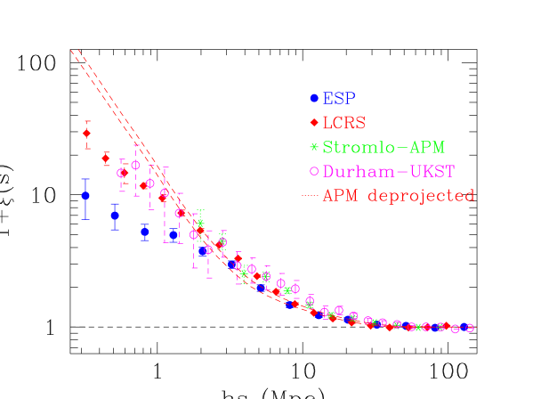
Figure 6: The function $1+\xi(s)$ for the same surveys of Figure 2. A stable power–law scaling would indicate a fractal range. It is clear how peculiar motions, that affect all data plotted but the APM $\xi(r)$ which is computed in projection, do distort significantly the overall shape. What would seem to be an almost regular scaling range with $D\sim 2$ from 0.3 to 30 $h^{-1}\,{\rm Mpc}\;$, hides in reality a more complex structure, with a clear inflection around 3$h^{-1}\,{\rm Mpc}\;$, which is revealed only when redshift–space effects are eliminated.

Although the data available today have increased by an order of magnitude at least, the debate on the scaling properties and homogeneity of the Universe is still lively. Given the subject of these lectures and the extensive use we have made so far of correlation functions, I shall concentrate here on the evidences concerning points ii) and iii) in the summary list above. In Figure 6, I have plotted the function $1+\xi(s)$ for the same surveys of Figure 2. Taken at face value, the figure shows that the redshift survey data can be reasonably fitted by a single power law only out to $\sim 5\,h^{-1}\,{\rm Mpc}\;$. However, as soon as we compare these to the real–space $1+\xi(r)$ from the APM survey, we realize that what we are seeing here is dominated by the redshift–space distortions. In other words, a fractal dimension on small scales can only be measured from angular or projected correlations, and if the data are interpreted in this way, it is in fact close to $D\simeq 1.2$. Above $\sim 5\,h^{-1}\,{\rm Mpc}\;$, a second range follows where $D$ varies between 2 and 3, when moving out to scales approaching $100\,h^{-1}\,{\rm Mpc}\;$. The range between $5\,h^{-1}\,{\rm Mpc}\;$ and $\sim 30\,h^{-1}\,{\rm Mpc}\;$ can in principle be described fairly well by a fractal dimension $D\simeq 2$, as originally found in [14], a dimension that could perhaps be topological rather than fractal, reflecting a possible sheet–like organisation of structures in this range [33]. Above $100\,h^{-1}\,{\rm Mpc}\;$ the function $1+\xi(r)$ seems to be fairly flat, indicating a possible convergence to homogeneity. However, once this is established, this kind of plot does not allow one to evidence clustering signals of the order of 1%, which can only be seen when the contrast with respect to the mean is plotted, i.e. $\xi(s)$. For a similar analysis and more details, see the pedagogical paper by Martìnez [34].

Another way of reading the same statistics and on which I would like to give an update with respect to [31] is the scaling of the correlation length $r_{\circ}$ with the sample size. It is known that for too small samples there is indeed a growth of $r_{\circ}$ with the sample size (see e.g. early results in [35]). This is naturally expected: galaxies are indeed clustered with a power–law correlation function, and inevitably too small samples will tend statistically to overestimate the mean density, when measuring it in a local volume. When we consider modern samples, however, and we pay attention to not to compare apples with pears (galaxies with different morphology and/or different luminosity have different correlation properties, [31]), then the situation is more reassuring: Table 1 represents an update of that presented in [31], and reports the general properties of the four redshift surveys I have used so far as examples. Being the survey volumes not spherical, here the “sample radius” is defined as that of the maximum sphere contained within the survey boundaries (see [31]). All these are estimates of $r_{\circ}$ in real space.

Survey	$d$	$R_{s}$	$r_{\circ}$ (predicted)	$r_{\circ}$ (observed)
ESP	$\sim 600$	5	1.7	$4.50^{+0.22}_{-0.25}$
Durham/UKST	$\sim 200$	30	10	$4.6\pm 0.2$
LCRS	$\sim 400$	32	11	$5.0\pm 0.1$
Stromlo/APM	$\sim 200$	83	28	$5.1\pm 0.2$

Table 1: The behaviour of the correlation length $r_{\circ}$ for the surveys discussed in previous figures, compared to predictions of a $D=2$ model. All estimates of $r_{\circ}$ are in real space. $d$ is the effective depth of the surveys, while the “sample radius” $R_{s}$ has been computed as in [31]. All measures of distance are expressed in $\,h^{-1}\,{\rm Mpc}\;$.

The observed correlation lengths are significantly different from the values predicted by the simple $D=2$ fractal model. The result would be even worse using $D=1.2$. The bare evidence from Table 1 is that the measured values of $r_{\circ}$ are remarkably stable, despite significant changes in the survey volumes and shapes.

The counter–arguments in favour of a fractal interpretation of the available data are instead summarised in the chapter by M. Montuori. As the students can check, the main points of disagreement are related to a) the use of some samples whose incompleteness is very difficult to assess (as e.g. heterogeneous compilations of data from the literature), and b) the estimators used for computing the correlation function and the way they take the survey shapes into account. Also on these issues, the 2dF and SDSS surveys will provide data sets to fully clear the scene. In fact, preliminary estimates of the correlation function from the 2dF survey provide a result in good agreement with the analyses shown here [1].

4.3 Scaling in Fourier space

It is of interest to spend a few words on the complementary, very important view of clustering in Fourier space. The Fourier transform of the correlation function is the power spectrum $P(k)$

$$P(k)=4\pi\int_{0}^{\infty}\xi(r){\sin(kr)\over kr}r^{2}dr\,\,\,\,\,,$$ (18)

which describes the distribution of power among different wavevectors or modes $k=2\pi/\lambda$ once we decompose the fluctuation field $\delta=\delta\rho/\rho$ over the Fourier basis [4]. The amount of information contained in $P(k)$ is thus formally the same yielded by the correlation function, although their estimates are differently affected by the uncertainties in the data (e.g. [4, 36]).

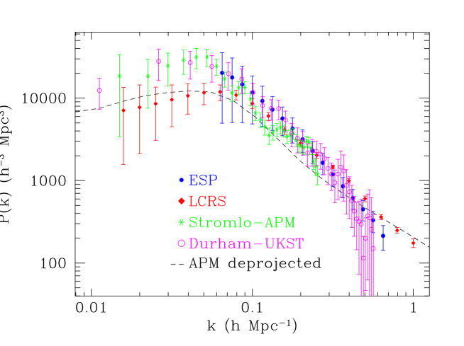
Figure 7: The power spectrum of galaxy clustering estimated from the same surveys of Figure 2 (also from [2], power spectrum estimates from [36, 37, 38, 39]). Also in Fourier space the differences between real– and redshift–space clustering are evident above $k\simeq 0.2\,h\,{\rm Mpc^{-1}}\;$.

One practical benefit of the description of clustering in Fourier space through $P(k)$ is that for fluctuations of very long spatial wavelength ($\lambda>100\,h^{-1}\,{\rm Mpc}\;$), where $\xi(r)$ is dangerously close to zero and errors easily make the measured values fluctuate around it (see Figure 2), $P(k)$ is on the contrary very large. Around these scales, most models predict a maximum for the power spectrum, the fingerprint of the size of the horizon at the epoch of matter–radiation equivalence. More technical details on power spectra can be found in the chapter by J. Peacock in this same book.

In Figure 7, I have plotted the estimates of $P(k)$ for the same surveys of Figure 2. Here again the projected estimate from the APM survey allows us to disentangle the distortions due to peculiar velocities, which have to be taken properly into account in the comparisons to cosmological models. Here scales are reversed with respect to $\xi(r)$, and the effect manifests itself in the different slopes above $\sim 0.3\,h\,{\rm Mpc^{-1}}\;$: an increased slope in real space (dashed line) corresponds to a stronger damping by peculiar velocities, diluting the apparent clustering observed in redshift space (all points). Below these strongly nonlinear scales, there is a good agreement between the slopes of the different samples (with the exception of the LCRS, see [36] for discussion), with a well–defined $k^{-2}$ power law range between $\sim 0.08$ and $\sim 0.3\,h\,{\rm Mpc^{-1}}\;$. The APM data show a slope $\sim k^{-1.2}$, corresponding to the $\gamma\simeq-1.8$ range of $\xi(r)$, while at smaller $k$’s (larger scales) they steepen to $\sim k^{-2}$, in agreement with the redshift–space points. It is this change in slope that produces the shoulder observed in $\xi(s)$ (cf. § 2). Peacock [40] showed that such spectrum is consistent with a steep linear $P(k)$ ($\sim k^{-2.2}$), the same value originally suggested to explain the shoulder when first observed in earlier redshift surveys [14]. A dynamical interpretation of this transition scale has been recently confirmed by a re–analysis of the APM data [41].

At even smaller $k$’s all spectra seem to show an indication for a turnover. However, when errors are checked in detail, they are at most consistent with a flattening, with the Durham–UKST survey providing possibly the cleanest evidence for a maximum around $k\sim 0.03\,h\,{\rm Mpc^{-1}}\;$ or smaller. A flattening or a turnover to a positive slope would be an indication for a scale over which finally the variance is close to or smaller than that of a random (Poisson) process. But we learn by looking at older data that a turnover can also be an artifact produced when wavelengths comparable to the size of the samples are considered, and here we are close to that case.

5 Do we really see homogeneity? Variance on $\sim$1000 h^-1 Mpc scales

Wu and collaborators [42] and Lahav [43] nicely reviewed the evidence for a convergence to homogeneity on large scales using several observational tests. On scales corresponding to spatial wavelengths $\lambda\sim 1000\,h^{-1}\,{\rm Mpc}\;$, the constraints on the mean–square density fluctuations are provided essentially by the smoothness in the X–ray and microwave backgrounds. Measuring directly the clustering of luminous objects over such enormous volumes, is only now becoming feasible. The 2dF survey will get close to these scales. The SDSS [26] will do even better through a sub–sample of early type galaxies selected as to reach a redshift $z\sim 0.5$. If the goal of a redshift survey is mapping density fluctuations on the larges possible scales a viable alternative to using single galaxies is represented by clusters of galaxies. Here I would like to discuss the properties of the largest of such surveys, that is in fact currently producing remarkable results on the amount of inhomogeneity on scales nearing 1000 $h^{-1}\,{\rm Mpc}\;$.

5.1 The REFLEX Cluster Survey

With mean separations $>10\,h^{-1}\,{\rm Mpc}\;$, clusters of galaxies are ideal objects for sampling efficiently long–wavelength fluctuations over large volumes of the Universe. Furthermore, fluctuations in the cluster distribution are amplified with respect to those in galaxies, i.e. they are biased tracers of large–scale structure: rich clusters form at the peaks of the large–scale density field, and their variance is amplified by a factor that depends on their mass, as it was first shown by Kaiser [44]. X–ray selected clusters have a further major advantage over galaxies or other luminous objects when used to trace and quantify clustering in the Universe: their X–ray emission, produced through thermal bremsstrahlung by the thin hot plasma permeating their potential well, is a good measure of their mass and this allows us to directly compare observations to the predictions of cosmological models (see [45] for a review, and [46] for a direct application).

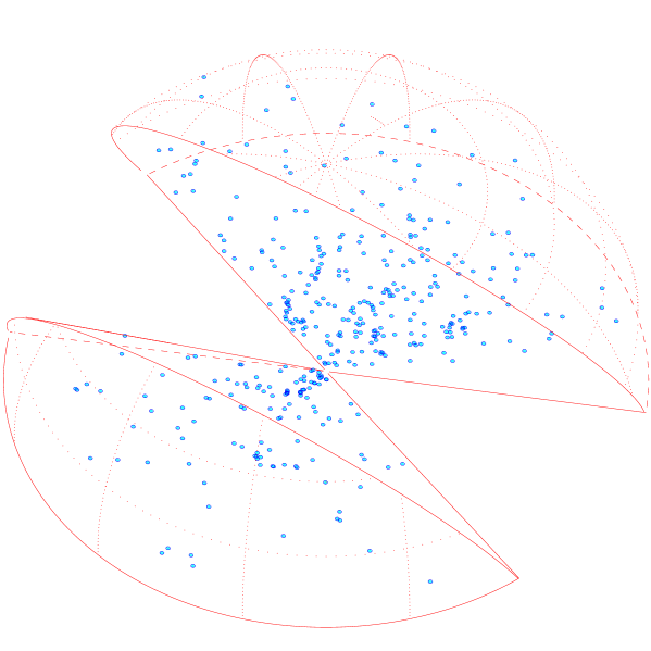
Figure 8: The spatial distribution of X–ray clusters in the REFLEX survey, out to 600 $h^{-1}\,{\rm Mpc}\;$. Note how, despite the coarser mapping of large–scale structure, filamentary superclusters (“chains” of clusters) are clearly visible.

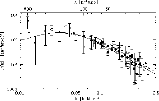
Figure 9: Estimates of the power spectrum of X–ray clusters from flux–limited sub–samples of the the REFLEX survey, framed within Fourier boxes of 300 (open squares), 400 (filled hexagons), and 500 (open hexagons) h^-1 Mpc side, containing 133, 188 and 248 clusters, respectively. The two lines correspond to the best–fitting parameters using a phenomenological shape with two power laws (solid), or a $\Lambda-$CDM model, with $\Omega_{M}=0.3$ and $\Omega_{\Lambda}=0.7$ (dashed) (from [46]).

The REFLEX (ROSAT-ESO Flux Limited X-ray) cluster survey is the result of the most intensive effort for a homogeneous identification of clusters of galaxies in the ROSAT All Sky Survey (RASS). It combines a thorough analysis of the X–ray data , and extensive optical follow–up with ESO telescopes, to construct a complete flux–limited sample of about 700 clusters with measured redshifts and X-ray luminosities [47, 48]. The survey covers most of the southern celestial hemisphere ($\delta<2.5^{\circ}$), at galactic latitude $|b_{II}|>20^{\circ}$ to avoid high absorption and stellar crowding. The present, fully identified version of the REFLEX survey contains 452 clusters and is more than 90% complete to a nominal flux limit of $3\times 10^{-12}$ erg s^-1 cm^-2 (in the ROSAT band, 0.1–2.4 keV). Mean redshifts for virtually all these have been measured during a long observing campaign with ESO telescopes. Details on the identification procedure and the survey properties can be found in [49], while earlier results are reported in [50, 51].

Figure 8 shows the spatial distribution of REFLEX clusters, evidencing a number of superstructures with sizes $\sim 100\,h^{-1}\,{\rm Mpc}\;$. One of the main motivations for this survey was to compute the power spectrum on extremely large scales, benefiting of the efficiency of cluster samples to cover very large volumes of the Universe. Figure 9 shows the estimates of $P(k)$ from three subsamples of the survey (from [46]).

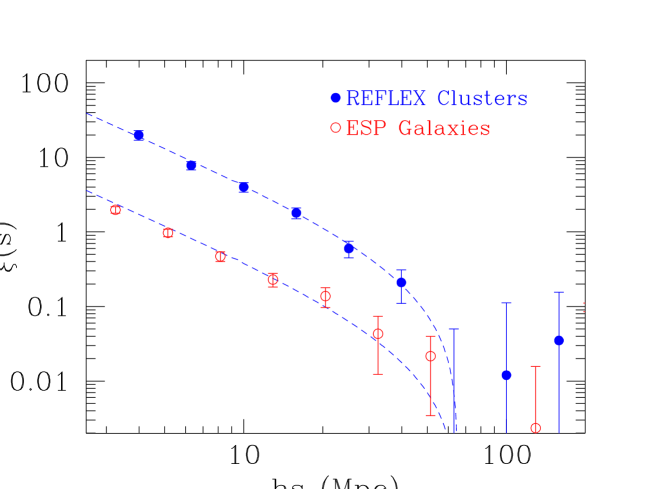
Figure 10: The two–point correlation function of the whole flux–limited REFLEX cluster catalogue (filled circles, [52]), compared to that of ESP galaxies (open circles, [9]. The dashed lines show the Fourier transform of a phenomenological fit to $P(k)$ which tries to include the large–scale power seen from the largest subsamples (top line). The bottom curve is that obtained after scaling down by an arbitrary bias factor ($b_{c}^{2}=(3.3)^{2}$ in this specific case).

One of the strong advantages of working with X–ray selected clusters of galaxies is that connection to model predictions is far less ambiguous than with optically–selected clusters (e.g. [53, 45]). We have therefore used the specific REFLEX selection function (converted essentially to a selection in mass), to determine that a low–$\Omega_{M}$ model (open or $\Lambda$–dominated), best matches both the shape and amplitude (i.e. bias value) of the observed power spectrum [46] (dashed line in the figure). In fact, the samples shown here do not reach the maximum spatial wavelengths we can possibly sample with the current data, as the Fourier box could be made to be as large as 1000 h^-1 Mpc (the survey reaches $z=0.3$ with the most luminous objects). In such case, however, our control over systematic effects becomes poorer, and work is currently undergoing to pin errors down and understand how trustable are our results on $\sim 1$ Gpc scale, where we do see extra power coming up. At the very least, REFLEX is definitely showing more clustering power on very large scales than any galaxy redshift survey to date. Similar hints for large–scale inhomogeneities seem to be suggested by the most recent analysis of Abell–ACO samples [54].

For $k>0.05\,h\,{\rm Mpc^{-1}}\;$, on the other hand, a comparison of REFLEX to galaxy power spectra shows a rather similar shape. This is probably better appreciated by looking at the two–point correlation function $\xi(s)$ [52], compared in Figure 10 to that of the ESP galaxy redshift survey. The agreement in shape between galaxies and clusters is remarkable on all scales, with a break to zero around $60-70\,h^{-1}\,{\rm Mpc}\;$ for both classes of objects. This is in general expected in a simple biasing scenario where clusters represent the high, rare peaks of the mass density distribution. This result strongly corroborates the simpler, reassuring view that at least above $\sim 5\,h^{-1}\,{\rm Mpc}\;$ the galaxy and mass distributions are linked by a simple constant bias.

5.2 “Peaks and Valleys” in the Power Spectrum

Most of the discussion so far has been concentrating on the beauty of finding “smooth” simple shapes for $\xi(r)$ or $P(k)$, as symptoms of an underlying order of Nature. Rather than being a demonstration of Nature inclination for elegance, however, this smoothness and simplicity might simply indicate our ignorance and lack of data. In fact, while smooth power spectra are predicted in models dominated by non–interacting dark matter particles, as Cold Dark Matter, a very different situation is expected in cases where ordinary (baryonic) matter plays a more significant role, with wiggles appearing in $P(k)$ that would be difficult to detect with the size and “Fourier resolution” of our current data sets.

The possibility that the power spectrum shows a sharp peak (or more peaks) around its maximum has been suggested a few times during the last few years. For example, Einasto and collaborators [55] found evidence for a sharp peak around $k\simeq 0.05\,h\,{\rm Mpc^{-1}}\;$ in the power spectrum of an earlier sample of Abell clusters, a feature later confirmed with lower significance by a more conservative analysis of the same data [56]. The position of this feature is remarkably close to the $\sim 130\,h^{-1}\,{\rm Mpc}\;$ “periodicity” revealed by Broadhurst and collaborators in a “pencil–beam” survey towards the galactic poles [57], and more recently, in an analysis of the redshift distribution of Lyman–break selected galaxies [58]. Other evidences have been claimed from two–dimensional analyses of redshift “slices” [59], or QSO superstructures [60].

These observations have stimulated some interesting work on models with high baryonic content. In this case, the power spectrum can exhibit a detectable inprint from “acoustic” oscillations within the last scattering surface at $z\sim 1000$, the same features observed in the Cosmic Microwave Background (CMB) radiation ([61]). While the most recent estimates of the REFLEX power spectrum do not show clear features around the scales of interest to justify “extreme” high–baryon models (contrary to early indications [62], which shows the importance of the careful assessment of errors), the extra power below $k\sim 0.02$ could still be an indication of an higher–than–conventional baryon fraction [61, 63], along the lines that seem to be suggested by the Boomerang CMB results [64].

6 Conclusions

At the end of these lectures, a student is possibly more confused than he/she was in the beginning, at least after a first read. I hope however that once the dust settles, a few important points emerge. First, that the processes which shaped the large–scale distribution of luminous objects we observe today are different at different scales. At small scales, we observe essentially the outcome of fully nonlinear gravitational evolution that re–shaped the linear power spectrum into a collection of virialised, or nearly so structures. Therefore, one cannot naively take the redshift survey data and look for specific patterns or statistical properties without taking into account galaxy peculiar motions. For this reason, one should be careful in over–interpreting things like a single power–law scaling from scales of a tenth of a Megaparsecs to hundred Megaparsecs, because, again, different phenomena are being compared. On the contrary, one can use these distortions to really “see” how the true mass distribution is, and I have spent a considerable part of these lectures to describe some of the techniques in use. Moving to larger and larger scales, we enter a regime where we are lucky enough that we can still see something related to the original scaling law of fluctuations. This is what was originally produced by some generator in the early Universe (inflation?) and processed through a matter (dark plus baryons) controlled amplifier. On even larger scales, we hope we are finally entering a regime where the variance in the mass is consistent with a homogeneous distribution, although we have seen that even the largest galaxy and cluster samples are barely sufficient to see hints of that, perhaps suggesting even more inhomogeneity than we expect. Does this mean that we are living in a pure fractal Universe? The scaling behaviour of galaxies and the stability of the correlation length seem to imply that this cannot be the case. On top of everything, the smoothness of the Cosmic Microwave Background (treated elsewhere in this book) is probably the most reassuring observation in this respect. What we seem to understand is that our samples have still difficulty to properly sample the very largest fluctuations of the density field, on scales where this is not fully Poissonian (or sub–Poissonian) yet.

Finally, I hope the students get the message that despite the tremendous progress of the last 25 years which transformed Cosmology into a real science, we still have a number of fascinating questions to answer and still feel far away from convincing ourselves that we have understood the Universe.

References

- [1] Colless M 1999 proc. of II Coral Sea Workshop http://www.mso.anu.edu.au/DunkIsland/Proceedings/
- [2] Guzzo L 1999 Proc. of XIX Texas Symposium on Relativistic Astrophysics E Aubourg et al.eds Nucl. Phys. B Proc. Suppl. CDR-09/06 (astro-ph/9911115)
- [3] http://www.mso.anu.edu.au/2dFGRS/
- [4] Peacock J A 1999 Cosmological Physics (Cambridge: Cambridge University Press)
- [5] Peebles P J E 1980 The Large–Scale Structure of the Universe (Princeton: Princeton University Press)
- [6] Maddox S J, Efstathiou G, Sutherland W J and Loveday J 1990 Mon. Not. R. Astr. Soc. 242 43p
- [7] Heydon–Dumbleton N H, Collins C A and MacGillivray H T 1989 Mon. Not. R. Astr. Soc. 238 379
- [8] Davis M and Peebles P J E 1983 Astrophys. J. 267 465
- [9] Guzzo L, Bartlett J, Cappi A et al.(ESP Team) 2000 Astron. Astrophys. 355 1
- [10] Tucker D.L., Oemler A., Kirshner R.P. et al.1997 Mon. Not. R. Astr. Soc. 285 L5
- [11] Loveday J, Peterson B A, Efstathiou G and Maddox S J 1992b Astrophys. J. 390 338
- [12] Ratcliffe A, Shanks T, Broadbent A et al.1996 Mon. Not. R. Astr. Soc. 281 L47
- [13] Baugh C M 1996 Mon. Not. R. Astr. Soc. 280 267
- [14] Guzzo L, Iovino A, Chincarini G et al.1991 Astrophys. J. 382 L5
- [15] Fisher K B, Davis M, Strauss M A et al.1994a Mon. Not. R. Astr. Soc. 266 50
- [16] Guzzo L, Strauss M A, Fisher K B, et al.1997 Astrophys. J. 489 37
- [17] Ratcliffe A, Shanks T, Parker Q A and Fong D 1998 Mon. Not. R. Astr. Soc. 296 173
- [18] Fisher K B, Davis M, Strauss M A et al.1994b 267 927
- [19] Fisher K B 1995 Astrophys. J. 448 494
- [20] Sheth R K, Hui L, Diaferio A and Scoccimarro R 2000 Mon. Not. R. Astr. Soc. (submitted astro-ph/0009167)
- [21] Peebles P.J.E. 1976 Astroph. and Space Sc. 45 3
- [22] Zurek W, Quinn P J, Warren M S and Salmon JK 1994 Astrophys. J. 431 559
- [23] Marzke R O, Geller M J, da Costa L N and Huchra J P 1995 Astron. J. 110 477
- [24] Landy S D, Szalay A S, and Broadhurst T J 1998 Astrophys. J. 494 L133
- [25] Quarello S and Guzzo L 2000 Clustering at high redshift A Mazure O Le Fèvre and V Le Brun eds. ASP Conf. Series 200 p 446
- [26] Margon B 1998 Phil. Trans. R. Soc. Lond. A (astro-ph/9805314)
- [27] Mandelbrot B B 1982 The Fractal Geometry of Nature (San Francisco: Freeman)
- [28] Pietronero L 1987 Physica 144A 257
- [29] Davis L in Critical Dialogues in Cosmology N Turok ed (Singapore: World Scientific) p 13
- [30] in Critical Dialogues in Cosmology N Turok ed (Singapore: World Scientific) p 24
- [31] Guzzo L 1997 New Astronomy 2 517
- [32] Provenzale A 1991 Applying fractals in Astronomy A Heck and J Perdang eds (Berlin: Springer)
- [33] Provenzale A, Guzzo L and Murante G 1994 Mon. Not. R. Astr. Soc. 266 555
- [34] Martìnez V 1999 Science 284 445
- [35] Einasto J, Klypin A and Saar E 1986 Mon. Not. R. Astr. Soc. 219 457
- [36] Carretti E, Bertoni C. Messina A et al.2000 Mon. Not. R. Astr. Soc. in press (astro-ph/0007012)
- [37] Lin H, Kirshner R P, Shectman S A et al.1996 Astrophys. J. 471 617
- [38] Tadros H and Efstathiou G P 1996 Mon. Not. R. Astr. Soc. 282 138
- [39] Hoyle F, Baugh C M, Ratcliffe A and Shanks T. 1999 Mon. Not. R. Astr. Soc. 309 659
- [40] Peacock J A 1997 Mon. Not. R. Astr. Soc. 284 885
- [41] Gaztañaga E and Juszkiewicz R 2000 Mon. Not. R. Astr. Soc. (submitted astro-ph/0007087)
- [42] Wu K K S Lahav O and Rees M J 1999 Nature 225 230
- [43] Lahav O 2000 Proc. of NATO-ASI Cambridge July 1999 R Critenden and N Turok eds (Dordrecht: Kluwer) (in press astro-ph/0001061)
- [44] Kaiser N 1984 Astrophys. J. 284 L9
- [45] Borgani S and Guzzo L Nature (in press)
- [46] Schuecker P, Böhringer H, Guzzo L et al.(REFLEX Team) Astron. Astrophys. (accepted)
- [47] Böhringer H, Guzzo L, Collins, C A et al.(REFLEX Team) 1998 The Messenger 94 21 (astro-ph/9809382)
- [48] Guzzo L, Böhringer H, Collins, C A et al.(REFLEX Team) 1999 The Messenger 95 27
- [49] Böhringer H, Guzzo L, Collins, C A et al.(REFLEX Team) 2000 Astron. Astrophys. (submitted)
- [50] De Grandi S, Guzzo L, Böhringer H et al.(REFLEX Team) 1999 Astrophys. J. 513 L17
- [51] De Grandi S, Böhringer H, Guzzo L et al.(REFLEX Team) 1999b Astrophys. J. 514 148
- [52] Collins C A, Guzzo L, Böhringer H et al.(REFLEX Team) 2000 Mon. Not. R. Astr. Soc. 319 939
- [53] Moscardini L, Matarrese S, Lucchin F and Rosati P 2000 Mon. Not. R. Astr. Soc. 316 283
- [54] Miller C J and Batuski D J 2000 Astrophys. J. (submitted astro-ph/0002295)
- [55] Einasto J, Einasto M, Gottloeber S et al.1997 Nature 385 139
- [56] Retzlaff J, Borgani S, Gottlober S et al.1998 New Astr. 3 631
- [57] Broadhurst T J, Ellis R S, Koo D C and Szalay A S 1990 Nature 343 726
- [58] Broadhurst T J and Jaffe A H 1999 Astrophys. J. (submitted astro-ph/9904348)
- [59] Landy D S, Shectman S A, Lin H et al.1996 Astrophys. J. 456 L1
- [60] Roukema B F and Mamon G 2000 Astron. Astrophys. (submitted astro-ph/0010511)
- [61] Eisenstein D J, Hu W, Silk J and Szalay A S 1998 Astrophys. J. 494 L1
- [62] Guzzo L 1999 in proc. of II Coral Sea Workshop http://www.mso. anu.edu.au/DunkIsland/Proceedings/
- [63] Guzzo L, Collins C A, Schuecker P et al.(REFLEX Team) 2001 (in preparation)
- [64] De Bernardis P, Ade P A R, Bock J J et al.2000 Nature 404 955