A probabilistic formulation for Empirical Population Synthesis: Sampling methods and tests

Abstract

We revisit the classical problem of synthesizing spectral properties of a galaxy using a base of star clusters, approaching it from a probabilistic perspective. The problem consists of estimating the population vector ${\bf x}$, composed by the contributions of $n_{\star}$ different base elements to the integrated spectrum of a galaxy, and the extinction $A_{V}$, given a set of absorption line equivalent widths and continuum colors. The formalism is applied to the base of 12 elements defined by Schmidt et al. (1991) as corresponding to the principal components of the original base employed by Bica (1988), and subsequently used in several studies of the stellar populations of galaxies. The exploration of the 13-D parameter space is carried out with a Markov chain Monte Carlo sampling scheme based on the Metropolis algorithm. This produces a smoother and more efficient mapping of the $P({\bf x},A_{V})$ probability distribution than the traditionally employed uniform-grid sampling.

This new version of Empirical Population Synthesis is used to investigate the ability to recover the detailed history of star formation and chemical evolution using this spectral base. This is studied as a function of (1) the magnitude of the measurement errors and (2) the set of observables used in the synthesis. Extensive simulations with test galaxies are used for this purpose. Emphasis is put on the comparison of input parameters and the mean ${\bf x}$ and $A_{V}$ associated with the $P({\bf x},A_{V})$ distribution. It is found that only for extremely low errors ($S/N>300$ at 5870 Å) all 12 base proportions can be accurately recovered, though the observables are recovered very precisely for any $S/N$. Furthermore, the individual $\overline{\bf x}$ components are biased in the sense that components which carry a large fraction of the light tend to share their contribution preferably among components of same age. Old, metal poor components can also be confused with younger, metal rich components due to the age $\times$ metallicity degeneracy. These compensation effects are linked to noise-induced linear dependences in the base, which very effectively redistribute the likelihood in ${\bf x}$-space. The age distribution, however, can be satisfactorily recovered for realistic $S/N$ ($\sim 30$). We also find that synthesizing equivalent widths and colors produces better focused results that those obtained synthesizing only equivalent widths, despite the inclusion of the extinction as an extra parameter.

1 Introduction

The stellar populations of galaxies carry a record of their star-forming and chemical histories, from the epoch of formation to the present. Their study thus provide a powerful tool to explore the physics of galaxy formation and evolution. Despite the detailed understanding of stellar evolution and of the properties of single stellar populations such as star clusters achieved over the past century, uncovering the history of galaxies through the study of their integrated light has proven to be a difficult problem (Pickles 1985; Worthey 1994 and references therein).

Two global approaches have been developed to tackle this issue. The first of these is Evolutionary Population Synthesis, which performs ab initio calculations of the spectral evolution of galaxies on the basis of stellar evolution theory, stellar spectral libraries, and prescriptions for the initial mass function, star formation rate and chemical evolution (Tinsley 1972; Larson & Tinsley 1974, 1978; Guiderdoni & Rocca-Volmerange 1987; Fioc & Rocca-Volmerange 1997; Charlot & Bruzual 1991; Bruzual & Charlot 1993; Leitherer et al. 1996, 1999 and references therein). The other approach is Empirical Population Synthesis (EPS hereafter), also known as ‘Stellar Population Synthesis with a Database’, which uses observed properties of stars or star clusters as a base on which to decompose the population mix in galaxy spectra (Spinrad & Taylor 1971; O’Connell 1976; Faber 1972; Pickles 1985; Bica 1988; Pelat 1997, 1998; Boisson et al. 2000). Of particular interest is the EPS method of synthesizing the spectra of galaxies using a base of star clusters. Perhaps the most appealing property of this method is the fact that the results do not hinge on assumptions about stellar evolution tracks nor initial mass functions, as these are ‘mother nature given’ in the empirically built base spectra. This technique has been pioneered by the work of Bica (1988, hereafter B88), where the stellar content of a large sample of galaxies was synthesized using the spectral base of star clusters described in Bica & Alloin (1986a, 1986b, 1987). Since then, several studies made use of this technique (Schmidt, Bica & Dottori 1989; Bica, Alloin & Schmidt 1990; Jablonka, Alloin & Bica 1990; Schmidt, Bica & Alloin 1990; Jablonka & Alloin 1995; De Mello et al. 1995; Bonatto et al. 1996, 1998, 1999, 2000; Schmitt, Storchi-Bergmann & Cid Fernandes 1999; Kong & Cheng 1999; Raimann et al. 2000).

In its original version (B88), this method made use of a large base of $n_{\star}=35$ elements, combined in different proportions ($x_{i}$; $i=1\ldots 35$) to synthesize a number of equivalent widths ($W$) of conspicuous absorption features. An uniform sweep of the parameter space along paths consistent with simple predefined chemical evolution scenarios was performed, and all combinations which produced $W$’s within 10% of the observed values were considered ‘solutions’. The final population vector ${\bf x}$ was taken to be the arithmetic mean of all such sampled solutions.

One of the main concerns raised by B88 method is that of the uniqueness of the solution, as first discussed by Schmidt et al. (1991, hereafter S91). With a 35-D population vector and at most 9 $W$’s to be synthesized, one has a highly degenerate algebraic system. As shown by S91, however, the original base was highly redundant, with several linearly dependent elements, and others which were practically so, as deduced by a principal component analysis. S91 then proposed the use of a reduced base of 12 elements. S91 also criticized B88’s uniform sampling of the ${\bf x}$ space (a ‘discrete combination procedure’ in their terms) and the use of a ‘mean solution’. Instead, they developed a constrained minimization procedure, which, as shown by their simulations with test galaxies built out of the base, is able to retrieve with good accuracy the correct population vector. Another difference of the S91 method compared to B88 is the possibility to search for solutions along the entire age $\times$ metallicity plane. B88 assumed that the chemical enrichment of the galaxy occurred during its formation ($\sim 10$ Gyr ago), with all stars younger than that having the same $Z$ as the oldest most metal rich component. Although this may be a reasonable approximation for the nuclear region of isolated galaxies, it does not allow for the effects of mergers, inflows or outflows, and is not applicable to high redshift sources, where the spectra usually integrate over the entire galaxy, including regions with different star formation and chemical histories (Jablonka et al. 1990; Jablonka & Alloin 1995).

The next improvement in this technique was the introduction of continuum colors in the synthesis. This was done by Schmitt, Bica & Pastoriza (1996), who, as B88, use a discrete combination procedure search for acceptable solutions, sweeping the parameter space along chemical enrichment paths. This version of EPS has been used in several subsequent studies (Bonatto et al. 1996, 1998, 1999, 2000; Kong & Cheng 1999). Another step was taken by Bonatto, Bica & Alloin (1995), who extended the star cluster base to the space ultraviolet (1200–3200 Å). They too use an arithmetic average to represent the solution of the synthesis.

In two recent papers, Pelat revisited the EPS problem of synthesizing $W$’s using an elegant formalism based on convex algebra concepts. In Pelat (1998) he shows how the algebraic solution of the EPS problem can be narrowed down to a sub-space of ${\bf x}$ delimited by a set of ‘extreme-solutions’, any convex combination of which yields an exact solution in the underdetermined cases (more parameters than constraints). His results shed new light into the issue of algebraic degeneracy, which has always haunted EPS due to the widespread belief that with more parameters than observables one is bound to fit the data in one way or another. He proposes a quick test of whether the $W$’s of a galaxy are synthesizable by computing the region in $W$-space spanned by all physical combinations of the base elements. We verified that in the case of the 12 elements base used by S91 this region is narrow (Leão 2001), such that small measurement errors are enough to place objects outside this ‘synthetic domain’, hence preventing the existence of mathematically exact solutions. In real applications, one therefore expects the degeneracy of EPS to be more of a statistical nature than algebraic. In these cases, as well as in overdetermined problems, Pelat (1997) demonstrates that the best model is to be found along the boundary of the synthetic domain by minimizing an appropriately defined $\chi^{2}$-like distance. Uncertainties in the population vector can also be readily computed, as shown by Moultaka & Pelat (2000).

Boisson et al. (2000) recently applied Pelat’s method to a sample of 12 active galaxies from Serote Roos et al. (1998). They synthesize $n_{W}=47$ absorption lines with a base of $n_{\star}=30$ stars from the stellar spectral libraries of Serote Roos, Boisson & Joly (1996) and Silva & Cornell (1992). Their results nicely illustrate the power of this new EPS technique, which will certainly be extended to larger samples and other classes of galaxies in future studies. The B88 method and its variants, on the other hand, already have a large body of literature associated to it. Nevertheless, this popular and attractive EPS technique, while intuitively acceptable, has neither been adequately tested nor cast onto a sound mathematical formalism which supports its application. Furthermore, it gives no measure of the uncertainties or potential biases on the population vector, thus giving no simple way to prevent overinterpretations of the resulting population of the age $\times$ metallicity plane. These issues are the focus of the present paper.

Our main goals are to:

• Elaborate a mathematically consistent formulation of the EPS problem in the context of probability theory.

• Develop and test a sampling method to explore the parameter space in EPS problems. In particular, we aim to improve upon the Schmitt et al. (1996) technique of synthesizing both equivalent widths and colors, but within the context of a probabilistic formulation.

• Use the method to investigate the effects of measurement errors and of the specific set of observables used upon the results of the synthesis with the reduced B88 star cluster base described in S91. In particular, we wish to evaluate whether these factors introduce biases in the population mix inferred from this popular synthesis technique and at what level of detail can its results be trusted.

This paper is organized as follows: Item (i) of the above list is addressed in section 2. In section 3 we deal with point (ii). This is done by investigating the applicability of a Metropolis algorithm to sample the parameters probability distribution in EPS, and testing the method with simulations based on Bica’s spectral base. In section 4 we address item (iii) by means of extensive simulations which explore the ability to recover the detailed star-formation and chemical histories of galaxies with this base. Finally, section 5 summarizes our main results.

2 Formalism

2.1 Basic equations

EPS studies seek to find combinations of a spectral base which reproduce a given set of measured observables, often taken as the equivalent widths $W_{j}$ of $n_{W}$ conspicuous absorption features. The base consists of $n_{\star}$ elements representing well defined simple stellar populations such as star-clusters, with equivalent widths $W^{\star}_{ij}$ and corresponding continuum fluxes over the lines $F^{\star}_{ij}$ ($j=1,\ldots n_{W}$, $i=1,\ldots n_{\star}$) normalized at a reference wavelength. Denoting by $x_{i}$ the fractional contribution of the $i$-th base element to the total flux at the reference wavelength, one obtains a system of $n_{W}$ equations

$$W_{j}=W_{j}({\bf x})=\frac{\sum_{i=1}^{n_{\star}}W^{\star}_{ij}F^{\star}_{ij}x_{i}}{\sum_{i=1}^{n_{\star}}F^{\star}_{ij}x_{i}};~{}~{}~{}~{}j=1,...,n_{W}$$ (1)

for the synthetic $W$’s (e.g., Joly 1974). This set of constraints can be augmented by synthesizing $n_{C}$ observed continuum fluxes $C_{k}$ ($k=1,\ldots n_{C}$), provided allowance is made for reddening, here parametrized by the V-band extinction $A_{V}$. Assuming all $n_{\star}$ populations are equally reddened, one obtains

$$C_{k}=C_{k}({\bf x},A_{V})=g_{k}(A_{V})\sum_{i=1}^{n_{\star}}C^{\star}_{ik}x_{i};~{}~{}~{}~{}k=1,...,n_{C}$$ (2)

where a distinction is made between $C^{\star}$ and $F^{\star}$, since the $n_{C}$ fluxes to be synthesized need not correspond to the wavelengths of the $n_{W}$ absorption lines. We hereafter refer to the $C_{k}$’s as continuum colors, as they are in fact ratios of continuum fluxes with respect to the continuum at the normalization wavelength. The function $g_{k}(A_{V})$ reddens the normalized color at wavelength $\lambda_{k}$ by $A_{\lambda_{k}}$ according to a specified reddening law.

Finally, physical solutions must further satisfy the normalization and positivity constraints:

$$\sum_{i=1}^{n_{\star}}x_{i}=1;~{}~{}x_{i}\geq 0~{}{\rm for}~{}i=1,...,n_{\star},~{}{\rm and}~{}~{}A_{V}\geq 0.$$ (3)

The normalization condition effectively reduces one degree of freedom. When modeling colors, however, one has to introduce $A_{V}$ as a further parameter, so that the number of parameters still is $n_{\star}$.

2.2 Probabilistic formulation

The data ${\cal D}$ to be modeled are thus composed of a set of $n_{obs}=n_{W}+n_{C}$ observables. The measurement errors in each observable, collectively denoted by ${\bf\sigma}$, are assumed to be known. Given these, the problem of EPS is to estimate the population vector ${\bf x}$ and the extinction $A_{V}$ that ‘best’ represents the data according to a well defined probabilistic model. It is equally important to estimate the uncertainties in the parameters, as these prevent over-interpreting the resulting mixture of stellar populations at a level of detail not warranted by the data or by intrinsic limitations of the base.

The probability of a solution $({\bf x},A_{V})$ given the data ${\cal D}$ and the errors ${\bf\sigma}$, is given by Bayes theorem:

$$P({\bf x},A_{V}|{\cal D},{\bf\sigma},{\cal H})=\frac{P({\cal D}|{\bf x},A_{V},{\cal H})P({\bf x},A_{V}|{\bf\sigma},{\cal H})}{P({\cal D}|{\cal H})}.$$ (4)

${\cal H}$ summarizes the set of assumptions on which the inference is to be made. They include: the mapping between parameters and observables is given by eqs. (1) and (2); ${\bf x}$ and $A_{V}$ must satisfy the constraints expressed in eq. (3); the stellar population in the target galaxy is well represented by the base elements; the observational errors are Gaussian; the reddening law is known.

The likelihood $P({\cal D}|{\bf x},A_{V},{\bf\sigma},{\cal H})$ is a measure of how good (or bad) is the fitting to the data for model parameters ${\bf x}$ and $A_{V}$. Under the hypothesis of Gaussian errors, the probability of the data given the parameters is

$$P({\cal D}|{\bf x},A_{V},{\bf\sigma},{\cal H})\propto e^{-{\cal E}},$$ (5)

with ${\cal E}$ defined as half the value of $\chi^{2}$:

$${\cal E}({\bf x},A_{V}) = \frac{1}{2}\chi^{2}({\bf x},A_{V})=\frac{1}{2}\sum_{j=1}^{n_{W}}\left(\frac{W_{j}^{obs}-W_{j}({\bf x})}{\sigma(W_{j})}\right)^{2}$$

$$+\frac{1}{2}\sum_{k=1}^{n_{C}}\left(\frac{C_{k}^{obs}-C_{k}({\bf x},A_{V})}{\sigma(C_{k})}\right)^{2}$$

The likelihood, as the total $\chi^{2}$, separates into a $W$ and a color related term, of which only the latter depends on $A_{V}$.

The normalizing constant $P({\cal D}|{\cal H})$ in Bayes theorem (the ‘evidence of ${\cal H}$’) is irrelevant to the level of inference discussed here, i.e., the estimation of ${\bf x}$ and $A_{V}$. It can be used, for instance, to compare different spectral bases.

$P({\bf x},A_{V}|{\cal H})$ is the joint a priori probability distribution of ${\bf x}$ and $A_{V}$, and states what values the model parameters might plausibly take. For instance, physically acceptable population fractions should have priors that are zero in regions of the parameter space where the constraints of positivity and unit sum are not satisfied. A prior that is uniform on the parameters and includes these constraints is a non-informative prior, because it does not impose any constraints on the solutions besides those expressed by eq. (3). This is the prior that will be used in this work.

For a non-informative prior the posterior probability $P({\bf x},A_{V}|{\cal D},{\bf\sigma},{\cal H})$ is simply proportional to the likelihood:

$$P({\bf x},A_{V}|{\cal D},{\bf\sigma},{\cal H})\propto e^{-{\cal E}({\bf x},A_{V})}$$ (7)

This expression contains the full solution of the EPS problem, as embedded in it is not only the most probable model parameters but also their full probability distributions. Furthermore, projected posterior distributions for any of the $n_{\star}$ parameters can be obtained by marginalizing eq. (7) with respect to all other parameters. For instance, the probability density of proportion $x_{i}$ of the $i$-th base element is

$$P(x_{i}|{\cal D},{\bf\sigma},{\cal H}) = \int\ldots\int P({\bf x},A_{V}|{\cal D},{\bf\sigma},{\cal H})dx_{1}\ldots$$

$$dx_{i-1}dx_{i+1}\ldots dx_{n_{\star}}dA_{V}$$

and equivalently for $A_{V}$. Similarly, one can construct joint posteriors for, say, the total proportion of all base components of same age or $Z$, or for the mean age and $Z$ of the stellar population. This would of course provide a coarser description of a galaxy’s stellar content than the individual posteriors $P(x_{i}|{\cal D},{\bf\sigma},{\cal H})$, but that may be all that is possible under some circumstances, such as when only a reduced set of observables is available or when observational errors are large (section 4).

It is easy to see how the B88 and Schmitt et al. (1996) synthesis techniques fit into this general probabilistic formulation. By synthesizing the observables within $\sim 10\%$ ‘error boxes’, these authors implicitly assumed a box-car likelihood function $P({\cal D}|{\bf x},A_{V},{\bf\sigma},{\cal H})$, whereas by performing arithmetic means over all accepted $({\bf x},A_{V})$ combinations in a uniform grid they are implicitly sampling the corresponding posterior probability distributions. Also, the a priori constraints on the occupation of the age $\times$ $Z$ plane imposed by these authors (but relaxed in subsequent works) simply reflect their use of an informative prior. This gives some formal justification for their heuristically designed EPS method. It is therefore reasonable to expect that an implementation of EPS based on the formalism presented here should give results roughly compatible with those previously obtained. An uniform sweep of the (${\bf x},A_{V}$) space is however a very inefficient sampler for (2.2), so some improvement is needed there. This is discussed next.

3 Sampling Method and Tests

Despite its formal merits, at the computational level our probabilistic approach faces the same basic difficulty as previous EPS codes, namely, the high dimensionality of the problem. For spectral bases with astrophysically interesting resolution in age and metallicity the number of elements $n_{\star}$ quickly becomes large enough to render the exploration of the parameter space a non-trivial task. Before discussing methods to sample the (${\bf x},A_{V}$) space, we present the spectral base used in this work (§3.1) and describe how we deal with the uncertainties in the observables (§3.2).

3.1 The spectral base and observables

Base Elements Used
HII	10 Myr	100 Myr	1 Gyr	10 Gyr	log(Z/Z⊙)
	10	8	5	1	0.6
12	11	9	6	2	0.0
			7	3	-1.0
				4	-2.0

Table 1: Ages, metallicities and numbering convention for the star clusters in the base.

The base used for the synthesis here is that of S91. It contains $n_{\star}=12$ population groups, spanning five age bins—10 Gyr (which actually represent globular cluster-like populations), 1 Gyr, 100 Myr, 10 Myr and HII (corresponding to current star formation, and represented by a pure $F_{\lambda}\propto\lambda^{-2}$ continuum based on the spectrum of 30 Dor)—and four metallicities—0.01, 0.1, 1 and 4 Z_⊙ (Table 1). The observables in this base comprise the $n_{W}=9$ equivalent widths of the absorption lines CaII K $\lambda$3933, CN $\lambda$4200, G band $\lambda$4301, MgI $\lambda$5175, CaII $\lambda$8543, CaII $\lambda$8662, H$\delta$, H$\gamma$ and H$\beta$, as well as $n_{C}=7$ continuum fluxes at selected pivot wavelengths: 3290, 3660, 4020, 4510, 6630, 7520 and 8700 Å, all normalized to 5870 Å. According to Bica & Alloin (1986a, 1987) and Bica, Alloin & Schmitt (1994), the equivalent width windows and continuum points were defined based on very high signal to noise spectra of galaxies, with the express goal of using them to synthesize the stellar population of galaxies. These spectra were obtained by creating two average spectra, of blue and red galaxies, where the stellar population features can be clearly traced. The base values for these quantities have been previously published in Bica & Alloin (1986b, 1987) and Schmitt et al. (1996), and some were measured from data in Bica et al. (1994). These are recompiled in Table 2 , as they bear a direct impact on the analysis below. There are thus a maximum of $9+7=16$ observables to model with $n_{\star}=12$ parameters: $n_{\star}-1$ population fractions plus $A_{V}$. However, in several of the tests presented below we shall make use of a reduced subset of observables, as observational data sets seldom cover the whole spectral range spanned by this base.

According to Bica & Alloin (1986a, 1987) and Bica, Alloin & Schmitt (1994), since the ultimate goal of the continuum points and $W$’s is to synthesize the stellar population of galaxies, the $W$ windows and continuum points were defined based on very high signal to noise spectra of galaxies. These spectra were obtained by creating two average spectra, of blue and red galaxies, where the stellar population featuress can be identified.

The reddening of the colors is modeled with the extinction law described in Cardelli, Clayton & Mathis (1989, with $R_{V}=3.1$).

Equivalent Widths (Å)
#	K	CN	G	MgI	CaT1	CaT2	H$\delta$	H$\gamma$	H$\beta$
1	21.1	17.5	11.1	10.1	6.8	6.0	4.4	4.9	3.5
2	17.3	12.0	9.3	7.4	5.5	5.0	4.4	4.9	3.5
3	11.0	4.5	5.9	3.8	3.4	3.3	4.4	4.9	3.5
4	4.7	0.5	2.5	0.7	1.2	1.6	4.4	4.9	3.5
5	17.3	13.9	9.0	9.1	6.8	6.0	9.7	7.7	7.5
6	14.0	9.6	7.4	6.2	5.5	5.0	9.7	7.7	7.5
7	8.9	3.6	4.6	3.2	3.4	3.3	9.7	7.7	7.5
8	4.5	3.0	1.5	3.2	6.8	6.0	10.5	9.9	7.9
9	3.8	2.2	1.2	2.5	5.5	5.0	10.5	9.9	7.9
10	2.6	1.4	0.3	2.5	8.2	6.9	4.5	3.5	3.9
11	2.2	1.1	0.3	2.0	6.6	5.8	4.5	3.5	3.9
12	0.0	0.0	0.0	0.0	0.0	0.0	0.0	0.0	0.0
Continuum over the lines
1	0.34	0.48	0.55	0.87	1.03	1.04	0.44	0.58	0.79
2	0.48	0.59	0.65	0.90	0.96	0.96	0.56	0.67	0.83
3	0.72	0.78	0.81	0.95	0.84	0.84	0.76	0.82	0.91
4	0.94	0.96	0.97	1.01	0.72	0.71	0.96	0.97	1.00
5	1.03	1.05	1.06	1.04	0.70	0.70	1.05	1.06	1.06
6	1.03	1.05	1.06	1.04	0.70	0.70	1.05	1.06	1.06
7	1.03	1.05	1.06	1.04	0.70	0.70	1.05	1.06	1.06
8	1.89	1.75	1.68	1.23	0.59	0.58	1.79	1.65	1.38
9	1.89	1.75	1.68	1.23	0.59	0.58	1.79	1.65	1.38
10	1.55	1.34	1.27	1.06	0.95	0.94	1.40	1.25	1.08
11	1.55	1.34	1.27	1.06	0.95	0.94	1.40	1.25	1.08
12	2.34	2.03	1.93	1.37	0.40	0.38	2.11	1.90	1.56

Continuum Colors
#	3290	3600	4020	4510	6630	7520	8700
1	0.17	0.27	0.39	0.71	1.01	1.01	1.04
2	0.27	0.37	0.52	0.77	0.99	0.96	0.96
3	0.42	0.52	0.74	0.88	0.96	0.89	0.84
4	0.57	0.67	0.95	0.99	0.92	0.81	0.71
5	0.71	0.65	1.04	1.08	0.92	0.81	0.70
6	0.71	0.65	1.04	1.08	0.92	0.81	0.70
7	0.71	0.65	1.04	1.08	0.92	0.81	0.70
8	1.10	0.94	1.84	1.52	0.82	0.68	0.58
9	1.10	0.94	1.84	1.52	0.82	0.68	0.58
10	2.10	1.52	1.45	1.11	0.95	0.99	0.94
11	2.10	1.52	1.45	1.11	0.95	0.99	0.94
12	3.78	2.56	2.20	1.73	0.74	0.56	0.37

Table 2: Observables in the base, which make the matrices $W^{\star}_{ij}$, $F^{\star}_{ij}$ and $C^{\star}_{ij}$. All continuum fluxes are normalized to the continuum at 5870 Å.

3.2 Errors in the observables

The measurement errors in the observables play a key role in determining the structure of the likelihood function. Whereas such errors are available when analyzing observed galaxy spectra, they have to be postulated in the synthesis of test galaxies performed below. An alternative and potentially more attractive approach to deal with the errors is to marginalize eq. (2.2) over ${\bf\sigma}$. This yields more conservative estimates for the parameters, insofar as they are independent of the actual observational errors. In this paper we follow the traditional approach of treating ${\bf\sigma}$ as a relevant constraint in the synthesis process.

In order to insure a realistic correspondence between the values of the errors and the actual quality of the data we have adopted a prescription for the $\sigma$’s based on our experience in dealing with the measurement of $W$’s and $C$’s in galaxy spectra (Cid Fernandes, Storchi-Bergmann & Schmitt 1998). Two sources of uncertainty affect the measurements of $W$’s: (1) the noise within the line window, and (2) the uncertainty in the positioning of the pseudo-continuum fluxes $C_{k}$ at the pivot wavelengths, which affect $W_{j}$ because they define the continuum over the line. The effect of the first of these sources upon $\sigma(W_{j})$ is straight-forwardly obtained through standard propagation of errors by specifying the noise level at $\lambda_{j}$, the spectral resolution $\delta\lambda$, and the size $\Delta_{j}$ of the pre-defined window over which $W_{j}$ is measured. In Bica & Alloin (1986a) system the pseudo continuum is defined interactively by visual inspection of the spectrum around the pivot $\lambda$’s, which makes the estimation of $\sigma(C_{k})$ non straight-forward. In Cid Fernandes et al. (1998) we found these errors could be roughly scaled from the signal-to-noise ratio measured in nearby ‘line-free’ regions, such that the $S/N$ in the pseudo continuum is $(S/N)_{\rm PC}\sim\rho_{\rm PC}(S/N)_{\lambda}$, with $\rho_{\rm PC}\sim 2$–3. This leads to the following expression for the $\sigma(W_{j})$’s:

$$\sigma^{2}(W_{j})=\Delta_{j}\delta_{\lambda}(S/N)_{\lambda}^{-2}+(\Delta_{j}-W_{j})^{2}\rho_{\rm PC}^{-2}(S/N)_{\lambda}^{-2}$$ (9)

where the two terms correspond to the two sources of uncertainty discussed above. For simplicity, we further assume that the noise in the observed spectrum is constant for all $\lambda$’s, which results in $(S/N)_{\lambda}=C_{\lambda}(S/N)_{5870}$. The errors in the $C_{k}$’s thus become also constant:

$$\sigma(C_{k})=\rho_{\rm PC}^{-1}(S/N)_{5870}^{-1}$$ (10)

Besides yielding realistic values for the $\sigma$’s, this recipe has the advantage of quantifying the quality of the data in terms of a single quantity: The signal-to-noise ratio at the normalization wavelength 5870 Å. Of secondary importance are the spectral resolution and $\rho_{\rm PC}$, which in the simulations below are kept fixed at 5 Å and 3 respectively.

In order to provide a quantitative notion of how a value of $S/N$ translates into $\sigma(W_{j})$’s, we have computed these quantities for the observables corresponding to spectral groups S1 and S7 of B88, typical of the nuclei of early (red) and late (blue) type spiral galaxies respectively. For S1 our error recipe yields $\sigma(W_{\rm CaIIK})=36{\rm\AA}/(S/N)_{5870}$ and $\sigma(W_{\rm MgI})=19{\rm\AA}/(S/N)_{5870}$, so errors of $\sim 1$ Å or less are achieved with $(S/N)_{5870}\geq 30$. For S7 these lines have $\sigma(W)\sim 15{\rm\AA}/(S/N)_{5870}$.

3.3 Exploration of the parameter space: Sampling methods

The exploration of the (${\bf x},A_{V})$ space can be approached from two alternative perspectives: (1) A minimization problem, employing methods to search for the global $\chi^{2}$ minimum (maximum likelihood). Minimization techniques were explored in S91 and Pelat (1997) for the synthesis of $W$’s only. (2) A sampling problem, where one seeks to map out the posterior probability distribution (eq. 7).

The methods discussed in this paper are sampling methods, which do not explicitly search for a minimum. In the limit of small errors, however, one expects the posterior maps to peak at the most likely model. For large errors, on the other hand, the best model sampled may be well off the true global minimum, but in this case the probability distribution is so broad that the very meaning of ‘best model’ is questionable. In such cases it is arguably more important to estimate plausible ranges for the parameters than to carry out a refined search for the most likely values.

Our main motivation to explore the sampling approach is that most applications of EPS with Bica’s base to date focused on the estimation of mean parameters, whose meaning cannot be directly ascertained without estimating their uncertainty and/or biases. A critical re-evaluation of this method is thus crucial to establish to which level of detail the results of this popular technique can be trusted.

3.3.1 Uniform sampling

In order to compute the individual posterior probabilities for each parameter, we first note that eq. (2.2) for the $x_{i}$ posterior is simply the mean probability $P({\bf x},A_{V}|{\cal D},{\bf\sigma},{\cal H})$ over the space spanned by all possible values of $x_{j\neq i}$ and $A_{V}$ for a fixed $x_{i}$. The simplest method to compute such probabilities is to divide the (${\bf x},A_{V}$) space into a uniform grid with $\Delta x$ steps for the population fractions and $\Delta A_{V}$ for the reddening parameter. One then approximates eq. (2.2) by the finite sum

$$P(x_{i}|{\cal D},{\bf\sigma},{\cal H}) \simeq \frac{\sum_{s}e^{-{\cal E}({\bf x}_{s},A_{V,s})}\delta(x_{i}-x_{i,s})}{\sum_{s}e^{-{\cal E}({\bf x}_{s},A_{V,s})}}$$ (11)

where $s$ denotes a point (a ‘state’) in the 13-D grid and the $\delta(x_{i}-x_{i,s})$ term retains only those grid points where population $i$ contributes with fraction $x_{i}$ of the light.

This discrete sweeping of the parameter space is easy to implement, and was in fact the recipe followed by most works with Bica’s base to date (see section 1). A serious drawback of uniform sampling is its computational price. The number of grid cells is an extremely steep function of the resolution $\Delta x$. A coarse $\Delta x=10\%$ sampling yields $3.5\times 10^{5}$ ${\bf x}$-points, increasing to $\sim 8\times 10^{7}$ for $\Delta x=5\%$ and more than $4\times 10^{11}$ for a $2\%$ resolution! To obtain the grid size one has to further multiply these numbers by the number of points in the $A_{V}$ grid, whose limits have to be pre-defined. Schmitt et al. (1999), for instance, performed a synthesis study with $\Delta x=5\%$ and $\Delta A_{V}=0.06$ for $A_{V}$ between 0 and 1.5, which yields $2\times 10^{9}$ grid points, perhaps the finest grid ever used in EPS with this 12 elements base. One obviously always aim for the best resolution possible, but a priori estimates of what resolution is necessary are not straight-forward. A ‘good’ resolution should produce probability distributions that are smooth over scales of $\Delta x$ and $\Delta A_{V}$. The width of these distributions is of course a function of the observational errors and of the set of observables being synthesized.

3.3.2 Metropolis sampling

A further drawback of uniform sampling is that the algorithm spends most of the time in regions of negligible probability, which contribute little to the integral in equation (2.2), or its numerical version (eq. 11). A more efficient sweep of the parameter space would be to use a sampling scheme which traces the full probability distribution (eq. 7). One such ‘importance sampling’ scheme is the Metropolis algorithm (Metropolis et al. 1953), which samples preferentially regions where the posterior is large. This is the parameter-space exploration method adopted in this work.

Our implementation of the Metropolis sampler was as follows. Starting from an initial arbitrary point, at each iteration $s$ we pick one of the 13 variables at random and change it by an uniform deviate ranging from $-\epsilon$ to $+\epsilon$, producing a new state $s+1$. If the variable is one of the 12 $x_{i}$’s, the whole set is renormalized to unit sum. Moves towards unphysical values ($x_{i}<0$ or $>1$, $A_{V}<0$) were truncated. Downhill moves (i.e., towards smaller $\chi^{2}$) are always accepted, whilst changes to less likely states are accepted with probability $e^{-({\cal E}_{s+1}-{\cal E}_{s})}$, thus avoiding trapping onto local minima. This scheme, widely employed in statistical mechanics (Press et al. 1992; MacKay 2001 and references therein), produces a distribution which tends to the correct one as the number of samples $N_{s}$ increase. There is, however, no universal prescription to choose optimal values for $\epsilon$ or $N_{s}$, so some experimentation is needed.

3.4 Performance tests

In order to test our Metropolis EPS code we performed a series of simulations for artificial galaxies generated out of the base. Two sets of test galaxies were used. The first is composed of the 26 galaxies used by S91 (see their Table 5) to test their minimization algorithm. As they did not synthesize colors, we have used a fixed value of $A_{V}=2/3$ to redden all their galaxies. The second set is composed of 100 test-galaxies whose population vectors and extinctions were generated randomly using a scheme which insures that in many cases a few components dominate the light. All simulations presented in this paper were performed sampling $N_{s}=10^{8}$ states, with the ‘visitation parameter’ $\epsilon$ set to 0.005 for both the $x_{i}$’s and $A_{V}$. Experiments were also performed changing these quantities, and found to give nearly identical results. We note that less samples can be used if one is only interested in the mean (${\bf x},A_{V}$), as this naturally converges much faster than its full probability distribution. Simulations were performed for severals values of $(S/N)_{5870}$ and different sets of observables. Here we restrain the discussion to the illustration of the sampling method.

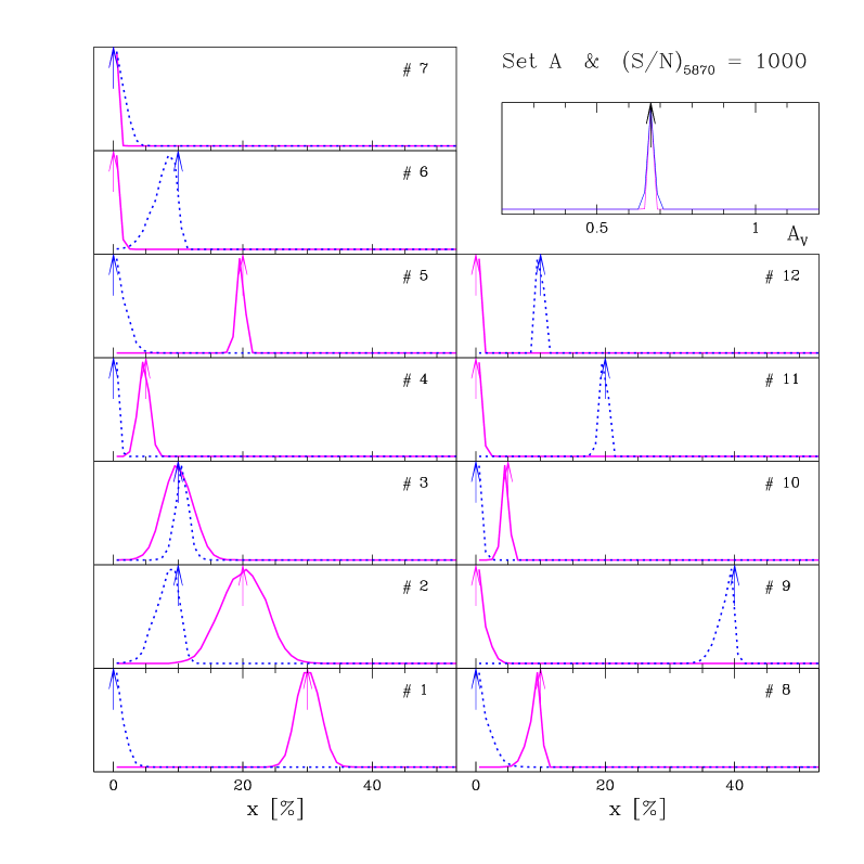
Figure 1: Individual posterior probability distributions for each of the components of the population vector ${\bf x}$ and the extinction, computed for an old population dominated test galaxy (solid lines) and a ‘younger’ galaxy (dotted lines). The top arrows indicate the input values of the corresponding parameter in each panel. The numbering of the ${\bf x}$ components follows the convention in Table 1. All 16 observables in Bica’s base (9 absorption lines $+$ 7 continuum points) were synthesized in this example and a S/N of 1000 was adopted to illustrate the convergence of the Metropolis sampler in the limit of (almost) perfect data.

In Fig. 1 we plot the individual projected posterior probability distributions for each of the 12 $x_{i}$’s plus $A_{V}$ for two of S91’s test galaxies composed of widely different stellar populations. The posteriors were computed synthesizing all 9 lines and 7 colors in the base (‘Set A’, as defined below) and using $(S/N)_{5870}=1000$ to define the errors in the observables. This is clearly an unrealistic, highly idealized situation, but it serves as a test-bed for the method in the limit of perfect data. The simulations were started from the $x_{i}=1/12$ and $A_{V}=0.5$ point. The plot shows that the posterior probabilities are sharp functions peaking at the expected input value, marked by upper arrows, demonstrating that the Metropolis sampler converges to the most likely region. One notes, however, that the strong components in the old age bin (such as $x_{1}$, $x_{2}$ and $x_{3}$ in the ‘old galaxy’ example, drawn as solid lines) have broader individual posteriors. This effect is further discussed in the next section.

In the opposite limit of large errors, $\sigma\rightarrow\infty$ (the ‘infinite temperature’ regime, as it would be called in statistical mechanics) the likelihood loses its discriminating power and becomes $\sim$ constant over the whole parameter-space. Eq. (2.2) then tends to $P(x_{i})\propto(1-x_{i})^{10}$ for a $n_{\star}=12$ base. In this regime the data does not constrain the model at all, and this expression for $P(x_{i})$ simply reflects the volume of the ${\bf x}$-space spanned by a given value of $x_{i}$. Not surprisingly, this distribution peaks at $x_{i}=0$, and has a mean value $\overline{x_{i}}=1/12$. We have verified that the Metropolis scheme recovers this distribution satisfactorily as $S/N\rightarrow 0$, which serves as a further test of the adequacy of this sampling method. The skewing of several of the individual posteriors plotted in Figs. 3 and 8 towards small $x_{i}$ is partly due to this effect, which drags the components to an intrinsically larger region of ${\bf x}$-space.

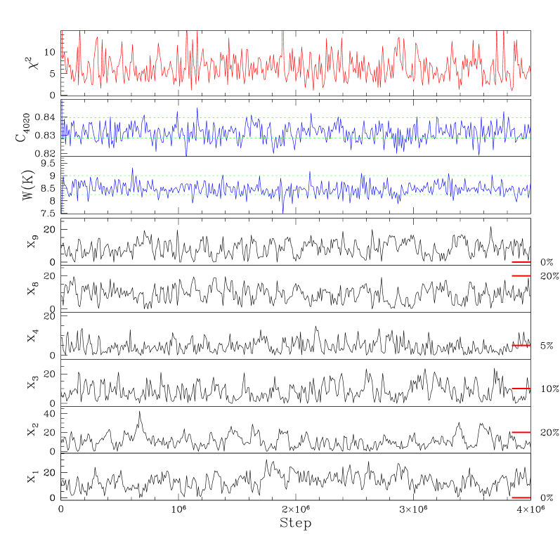
Figure 2: Illustration of the ‘step by step’ Metropolis walk through the parameter space. The six bottom panels illustrate the evolution of selected components of the population vector (in %), whose input $x_{i}$ values are indicated at the right edge of each plot. The values of the equivalent width of CaIIK and of the color $C_{4020}$ are plotted for each step in the third and second panels from the top. The dotted horizontal lines in these plots mark the $\pm 1\sigma$ range around the observed value. The top panel shows the $\chi^{2}$ for each sampled state. For clarity, only the first few million steps are show, and only 1 for every 10000 sampled states is actually plotted. All 16 observables in the base and $S/N=60$ were used in this example.

The evolution of the Metropolis walk through the 13-D (${\bf x},A_{V}$) space is illustrated in Fig. 2. For clarity, only 6 components of ${\bf x}$ and just one state for each $10^{4}$ steps are shown. Note that projected $P(x_{i})$ posteriors such as those in Fig. 1 are essentially histograms of the $x_{i}$ states sampled in walks as that in Fig. 2, but weighted by their $\exp-\chi({\bf x})^{2}/2$ likelihood. The input values of the components shown are indicated at the right edge of the plot for comparison. This particular example corresponds to a simulation with $S/N=60$ and with all 16 observables synthesized. One sees relatively large excursions of the parameters from their true values. Furthermore, anti-correlations between some of the components ($x_{1}$ and $x_{2}$, $x_{8}$ and $x_{9}$) are clearly visible. This ‘mirror effect’ becomes much more pronounced as $S/N$ increases, whereas for low $S/N$ the broadening of the likelihood function washes out such correlations. This is a consequence of redundancies between several of the base components, as further discussed below. The top panels in Fig. 2 show the evolution of the $\chi^{2}$ and how two of the synthesized observables, $W$(CaIIK) and $C_{4020}$, oscillate very much within their respective $\pm 1$ sigma error ranges. One therefore anticipates an excellent fit to the data, and indeed the $\chi^{2}$ obtained for the mean (${\bf x},A_{V})$ ‘solution’ in this example is just 0.8 (see also Fig. 7).

Overall, we conclude that the Metropolis algorithm is an efficient sampler of the parameter space for EPS problems. It provides a much more continuous mapping of ${\bf x}$ and $A_{V}$ than would be possible with a uniform grid. Furthermore, it is substantially more efficient computationally. A uniform grid with $10^{8}$ points would only sample each $x_{i}$ at $\sim 7\%$ steps and 10 values for $A_{V}$. By concentrating on the relevant regions of the parameter space, we achieve a much better resolution, as can be judged by the smoothness of the posterior distributions on scales of 1–2%.

One possible variation of this scheme is to combine the uniform grid and Metropolis routines, starting a Markov chain from each point on a uniform grid. Experiments with this alternative scheme were performed, and found to produce essentially the same results. This is to be expected, since we verified that the starting point has little effect upon the resulting posterior distributions. In fact, we performed a series of simulations using the input parameters as the starting point and obtained identical results. Though further improvements are possible, the simple Metropolis sampler already provides a substantial improvement over previous works with this base.

4 Tests of the base

Having developed a probabilistic formulation of EPS and a new sampling method, we now present a series of numerical experiments designed to evaluate the actual ability to recover the stellar population mix of galaxies using Bica’s base. The tests were performed with the same series of fictional galaxies described in section 3.4. Simulations were performed for $(S/N)_{5870}=10$, 30, 60, 100, 300 and 1000, and three different sets of observables:

• Set A: All 16 observables in the base.

• Set B: Only the 9 absorption line equivalent widths.

• Set C: The $W$’s of CaII K, CN, G-band and MgI+MgH plus the continuum fluxes at 3660, 4020, 4510 and 6630, all normalized to 5870 Å.

Set A is the ideal, as it uses all information in the base. Set B is used as a test of how much is actually gained by synthesizing colors as well as $W$’s, while Set C is composed of the observables used by Cid Fernandes et al. (1998) and Schmitt et al. (1999) to characterize the stellar content of active galaxies and their hosts through long-slit spectroscopy. These data will be used to perform a spatially resolved EPS study in a future communication.

4.1 Effects of the errors in the observables

We first investigate the effects of the measurement uncertainties in the observables upon the results of the synthesis. Qualitatively, one expects the degradation of the data quality to broaden the probability distributions. Furthermore, a shift and skewing of the $P(x_{i})$’s of intrinsically large components towards small $x_{i}$’s is also expected for low $S/N$ due to intrinsically larger number of states in this region of ${\bf x}$ (the ‘dragging effect’ discussed in §3.4). This is exactly what is observed in Fig. 3, where we overplot the individual posteriors for $S/N=1000$, 100 and 10 for one particular test galaxy of S91, synthesized with Set A observables. As in Fig. 1, the true parameters are indicated by the top arrows. The broadening of posteriors in this case can be safely attributed to the errors alone, since, as demonstrated by Pelat (1998) most of the test galaxies in S91 (including the one in Fig. 3) have a unique algebraic solution in a $W$-only EPS problem, despite the fact that the number of degrees of freedom (11 if we do not model the colors) falls short of the number of observables (9 $W$’s).

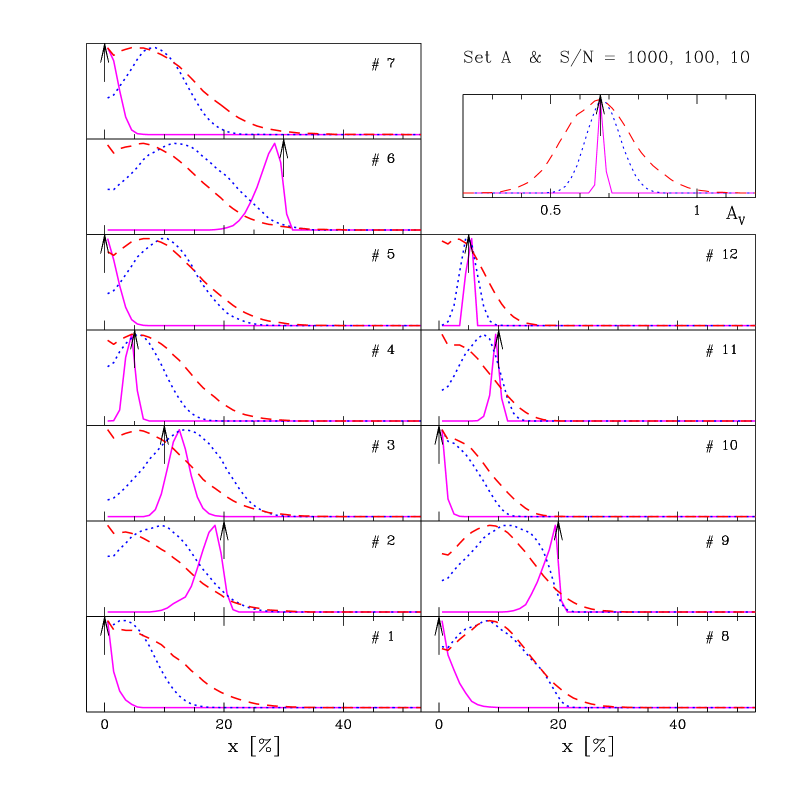
Figure 3: Effect of $S/N$ upon the individual probability distributions of the synthesis parameters for Set A observables. The different lines correspond to $S/N=1000$ (solid), 100 (dotted) and 10 (dashed). Notice how the probability of ${\bf x}$ components with a large contribution (like $x_{2}$, $x_{6}$ and $x_{9}$ in this example) are progressively redistributed among other components as the noise increases.

Figure 4: ‘Correlation Matrix’ for the test galaxy in Fig. 3. Each $x_{i}\times x_{j}$ panel shows one every 10000 of the first $10^{7}$ steps of a Metropolis run for $(S/N)_{5870}=300$ and Set A observables. The values at the bottom of each row indicate the input value of the corresponding component ($x_{1}=0$, $x_{2}=20\%$, …$x_{11}=10\%$, $x_{12}=10\%$). These are also indicated by the solid circles in each panel. Small and big tick marks are spaced by 2 and 10% respectively in all plots. Note the strong anti-correlations between adjacent components of same age.

Despite the large number of constraints in Set A, one sees that the individual posterior distributions are substantially broad even for a $S/N=100$ spectrum. The average standard deviation of the $x_{i}$’s for this combination of $S/N$ and observables is 3% over all simulations, but can reach more than 10% in individual components. Furthermore, the dominant components, 2, 6 and 9 in this example, are all badly affected by the errors. Fig. 3 shows that decreasing data quality progressively shifts $P(x_{2})$ towards smaller values, whereas the opposite happens with $x_{1}$. This compensation is also seen between components in the 1 Gyr ($x_{5}$, $x_{6}$ and $x_{7}$), 100 Myr ($x_{8}$ and $x_{9}$), and 10 Myr ($x_{10}$ and $x_{11}$) age bins and is the same ‘mirror’ effect observed before in Fig. 2. A compelling visualization of these compensations is given in Fig. 4, where we plot the individual Metropolis states for the test galaxy employed in Fig. 3 in a $x_{i}\times x_{j}$ matrix. The $S/N$ of 300 in this plot was chosen for clarity purposes; the same structure is present for other values, with the scatter around the strongest correlations increasing steadily as $S/N$ decreases, to the point that at $S/N=10$ the anti-correlations between components 1 and 2, or 8 and 9 become clouds similar to $x_{1}\times x_{5}$ in Fig. 4. All anticorrelations identified in Fig. 3 ($x_{1}\times x_{2}$, $x_{6}\times x_{5}$, etc.) are clearly represented in this graphical version of the correlation matrix.

These effects are rooted in the internal structure of the base. By definition, the base elements must be linearly independent, and the S91 base complies with this algebraic condition. Yet, some of its elements are practically linearly dependent, in the sense that combinations of other elements can recover them to a high degree of accuracy. As the noise increases, the residuals between representing an element by its exact $W$’s and $C$’s and a combination including other elements with more extreme values for the observables become statistically insignificant, explaining the compensations detected above. To demonstrate this we synthesized the base elements themselves with our code. Results for Set A observables and three different values of $S/N$ are shown in Fig. 5. Each panel corresponds to one of these 12 extreme test galaxies (labeled B1…B12), with the mean synthetic values of each of the components plotted along the vertical axis. The empty, shaded and filled histograms correspond to $S/N=100$, 30 and 10 respectively. Some of the components, most notably numbers 2, 3 and particularly 6, are synthesized with large contributions of others even for $S/N=100$. For the $x_{6}=100\%$ model (top left panel of Fig. 5), for instance, we find $\overline{x_{6}}=60\%$ for this high $S/N$, with 35 of the remaining 40% redistributed among components 5 and 7. Yet, the 16 observables are very well reproduced by this combination, with a total $\chi^{2}$ of just 3.8. This spreading of the light fractions becomes more pronounced for lower $S/N$’s, to the point that at $S/N=10$, components like 8 and 9, or 10 and 11 cannot be distinguished anymore, and end up dividing their contributions in roughly equal shares, with residuals spread over other components. The spread is much smaller in the synthesis of components 1, 4, 5 and 7, which represent extreme metallicities within age groups. For intermediate $Z$ systems (models B2, B3 and B6), however, these extreme components attract much of the percentage light contribution spilled over from neighboring populations of same age, so that their individual contributions in a real stellar population mix are as unreliable as the others.

This experiment demonstrates that for practical purposes the base is still linearly dependent, at least in a statistical sense, despite the effort of S91 in reducing the highly redundant original base of B88. This ‘noise-induced’, or ‘statistical linear dependence’, as we may call it, could indeed be inferred from the PCA analysis of S91, which showed that very little of the variance is associated with the last few eigenvectors. Within our probabilistic formulation, this ‘statistical linear dependence’ defines the structure of the likelihood function, which spreads first along directions in ${\bf x}$-space producing similar observables, carrying the mean ${\bf x}$ to more densely populated regions. This effect explains the redistribution of the probability observed in Figs. 3, 4 and all other simulations.

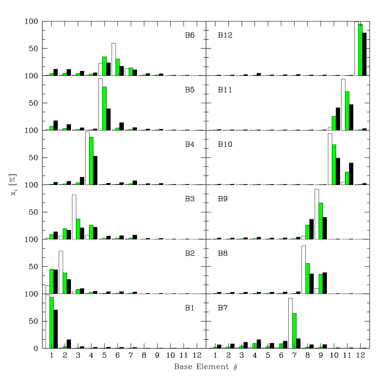
Figure 5: Synthesis of the base elements. Each panel shows the mean synthetic population vector (vertical axis) for 12 test galaxies whose 16 observables were generated with $x_{i}=100\%$, $i=1,\ldots 12$ (labeled B1…B12 respectively). Empty, shaded and filled histograms correspond to $S/N=100$, 30 and 10 respectively. Ideally, all histograms should be concentrated in the component used to generate the observables. In practice, some bases elements, most notably 2, 3 and 6, are well synthesized by combinations of others even for large $S/N$.

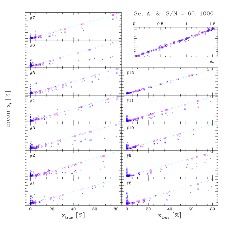
Figure 6: Input $\times$ output plots for all 13 individual parameters in the synthesis. Open circles map the results for Set A and $S/N=1000$, while crosses correspond to Set A and $S/N=60$. The output parameters are the mean values sampled from the global likelihood function. The dotted, diagonal lines in each panel mark the ‘input = output’ line. Error bars on the model parameters are not shown for clarity. Notice the systematic underestimation of large $x_{i}$’s and the corresponding overestimation of weak proportions for $S/N=60$.

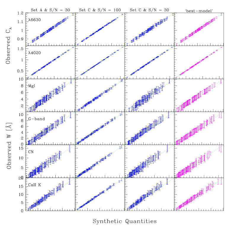
Figure 7: Input $\times$ output observables for a series of 100 test-galaxies synthesized with the Metropolis-EPS sampler. The three left columns of plots correspond to the three indicated combinations of the set of observables and $S/N$. For these plots the x-axis quantities were computed with the mean (${\bf x},A_{V}$) solution. The plots on the right column were made with Set C and $S/N=30$ (as those in the third column), but the synthetic observables in this cases were computed with the best model found during the Metropolis runs. Only the equivalent widths of four absorption features and two colors exhibited, but results for the remaining observables are equally good. The vertical and horizontal scales are the same for each panel, and the input $=$ output is indicated by a dotted line. Notice the excellent agreement, despite the fact that the input parameters are not accurately recovered by the synthesis process.

It is therefore extremely difficult to retrieve accurately all the input stellar population parameters even for excellent data. This is further illustrated in Fig. 6, where the input parameters are plotted against their mean values, as derived from the Metropolis runs. One hundred artificial galaxies are plotted in each panel, with open circles corresponding to Set A observables and $S/N=1000$, and crosses indicating the results for Set A and $S/N=60$. A systematic underestimation of strong components is seen for $S/N=60$, a good spectrum by any standard. This happens at the expense of an overestimation of the weaker components, which produces the large scatter seen in the bottom left corners of Fig. 6. The average uncertainties in the $x_{i}$’s are of order $\sigma(x_{i})\sim 3$–4% for $S/N=60$. These are not enough to account for the large differences between input and output $x_{i}$’s depicted in Fig. 6, so the errors induce a true bias in $\overline{\bf x}$. Note also that, in accordance with the discussion above, this bias is smaller for models with strong contributions of components 1, 4, 5 and 12, because of their extreme locations in the space of observables.

Only for unrealistically large $S/N$’s, which far exceed the quality of the data used to build the base in the first place, one is able to break the ‘statistical linear dependence’ of the base by distinguishing fine details in the observables. This should not be interpreted as a failure of the method, as what the code actually synthesizes are the observables! These are very precisely reproduced by the mean (${\bf x},A_{V}$), as illustrated in Fig. 7 for the $W$’s of CaII K, CN, G-band and MgI and two continuum colors. The remaining observables, not show in the figure, are equally well reproduced. Furthermore, whilst $S/N>300$ is needed to recover accurately the model parameters from the mean solution, the agreement between the synthetic and measured observables is excellent for any $S/N$. Obviously, an even better agreement is obtained if instead of $(\overline{\bf x},\overline{A_{V}})$ the best model sampled during the Metropolis excursion is used to reconstruct the observables, as illustrated in the fourth column of plots in Fig. 7 (see §4.5).

In conclusion, this comparison of input and output observables shows that the spreading of the probability and the confusion between components seen in Figs. 3 and 5 is not an artifact of the method, but a consequence of the internal structure of the spectral base. As found in other EPS studies (O’Connell 1996 and references therein) synthesizing the observables is one thing, but trusting the detailed star-formation history and chemical evolution implied by the synthesis is an altogether different story. On the positive side, a notable fact about Fig. 5 is that, consulting Table 1, one realizes that the reshuffling of the strength of the components occurs preferentially among populations of same age, an effect also clearly seen in Fig. 4. Though some redistribution among base elements of different age and $Z$ in the older 1 and 10 Gyr bins due to the age-$Z$ degeneracy also occurs, this indicates that the age distribution may be well recovered by the synthesis (§4.3).

4.2 Effects of different sets of observables

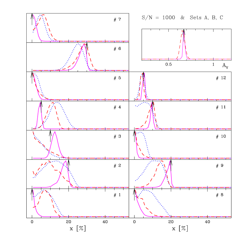
Figure 8: Analogous to Fig. 3, but exploring the effect of different sets of observables upon the synthesis parameters. Solid lines correspond to Set A (all observables), dotted lines to Set B (only 9 equivalent widths) and dashed lines to Set C (4 lines and 4 colors).

The effects of which set of observables is used in the synthesis are illustrated in Fig. 8, where results for Sets A, B and C for the same test galaxy as in Fig. 3 and $S/N=1000$ are compared. The figure shows that it is very advantageous to synthesize colors along with equivalent widths, despite the fact that one increases the dimensionality of the problem with the inclusion of $A_{V}$. This can be seen by comparing the performances of Sets A and B. The information contained in the colors not only improves the estimation of ${\bf x}$ but also allows a very good determination of $A_{V}$, which, unlike the population vector, is always well recovered by the synthesis.

Fig. 8 also shows how important it is to provide as many observational constraints as possible to constrain the synthesis, as Set A recovers the parameters much better than Sets B and C. Decreasing the number of observables in the synthesis thus have the same overall effect as decreasing the $S/N$. The width of the posteriors for Set C are partially attributed to the algebraic degeneracy in this set (8 observables and 12 degrees of freedom), which implies the existence of exact solutions in a sub-space of (${\bf x}$,$A_{V}$). That is not the case of Set A for the test galaxy in this example (Pelat 1998), but there, as for other sets, the ‘statistical linear dependence’ of the base is very efficient in spreading the likelihood even for such an idealized S/N ratio. The excellent agreement between the ‘observed’ and synthesized observables even for much worse S/N (Fig. 7) illustrates this point. Algebraic degeneracy is not as critical as the ‘statistical degeneracy’ induced by the combined effects of noise, limited data and the internal correlations in the base.

Studies which synthesize only $W$’s sometimes use the resulting population vector to compute a predicted continuum shape and derive $A_{V}$ a posteriori through the comparison with the observed continuum (e.g., B88; Boisson et al. 2000). From our Set B simulations, we find that this procedure yields values of $A_{V}$ 2–3 times less accurate than obtained with Set A. For $S/N=60$, for instance, Set A yields an rms dispersion in $A_{V}$ of 0.06 mag around the true value, whereas the dispersion for set B is 0.13 mag. Since this is a relatively small difference, these experiments validate the a posteriori computation of the extinction. Colors are more useful to constrain the population vector than to estimate $A_{V}$.

4.3 Age grouped results

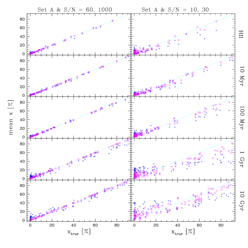
Figure 9: Age-binned light fractions in 100 input test galaxies versus the corresponding synthetic means. Left panels: Circles correspond to $S/N=60$, and crosses to $S/N=1000$, as in Fig. 6. Right panels: Circles correspond to $S/N=30$, and crosses to $S/N=10$. All results are for Set A observables.

The results of the tests above reveal a striking difficulty to accurately determine all 12 base components of Bica’s base in the presence of even very modest noise and/or when not all base observables are available for the synthesis. As indicated by the simulations, both the measurement errors and the use of reduced sets of observables act primarily in the sense of spreading a strong contribution in one component preferentially among base elements of same age. Grouping the population vector in age bins should thus produce more robust results. This expectation is confirmed in Fig. 9, where, analogous to what was done in Fig. 6, we plot the input values of the $x_{i}$’s against the output $\overline{x_{i}}$’s, but now for the five age binned groups, also for Set A simulations. The left panels correspond to the same values of $S/N$ used in Fig. 6, so that one can appreciate the enormous improvement achieved by grouping equal age elements. The right panels show that good results are also obtained for $S/N$ of 30 (circles), and that young populations ($\leq 100$ Myr) are reasonably well traced even for $S/N$ as low as 10 (crosses). Though some deviations survive, specially for the smaller $S/N$’s and the older age bins, the age-binned synthesis results are much more reliable than the results for the individual components, and, most importantly, do not require unrealistic $S/N$.

This conclusion also holds for Sets B and C, as illustrated in Fig. 10. Naturally, the restricted input data in these sets translates into a loss of information, and the agreement is not as good as for Set A. Note that Set C does a much better job in recovering populations of 100 Myr or less than Set B, a further example of how useful colors are in the synthesis. This happens because the color information (present in Set C but absent in B) impose stronger constraints on young populations than in older systems.

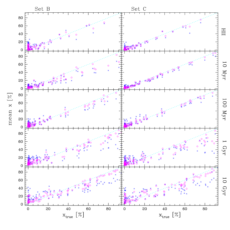
Figure 10: Input $\times$ output age binned ${\bf x}$ fractions for Set B (left) and Set C (right) observables. Circles correspond to $S/N=100$, and crosses to $S/N=30$.

The reliability of age-grouped proportions contrasts with the badly constrained and biased results for the individual components of ${\bf x}$, and is one of the main results of our study. This result puts in perspective all previous interpretations of the synthesis with this base. This fundamental limitation of the base was in fact previously known, but was never studied in detail. Schmitt et al. (1999), for instance, preferred to summarize the results of their synthesis study in terms of age grouped proportions for populations younger than 1 Gyr, in consonance with the results above. Still, in that work we kept a distinction between the different $Z$’s in the 10 Gyr age-group. At this level of detail the population fractions are very uncertain. In fact, since Set C observables and $S/N\sim 30$–60 were used in that study, Fig. 10 indicates that it would be safer to group their 1 and 10 Gyr proportions. Yet, the proportions for the younger ($\leq 100$ Myr) populations found by Schmitt et al. (1999), and which constituted the focus of that paper, are trustworthy (Fig. 10).

4.3.1 The age $\times$ metallicity degeneracy

A close inspection of the $S/N=10$ and 30 results in Fig. 9 reveals a compensation effect between the 1 and 10 Gyr age bins, albeit at a much smaller level than for the individual components (Fig. 6). This effect is much more pronounced in Sets B and C, as seen in Fig. 10.

The confusion between the 1 and 10 Gyr populations is related to the age-$Z$ degeneracy, which sets in precisely in this age range. This well known effect (O’Connell 1986, 1994; Worthey 1994) is also present in Bica’s base and affects the synthesis results. To visualize and quantify this effect we have computed the average log $Z$ and log age for both the input and synthetic ${\bf x}$ for our test galaxies. Given that ${\bf x}$ is a light fraction at 5870 Å, these averages ultimately represent flux-weighted ages and metallicities, which serve our current illustrative purposes, despite their ambiguous physical significance.

The ‘output - input’ $\log{\rm age}$ and $\log Z$ residuals are plotted against each other in Fig. 11. In these diagrams $\Delta\log{\rm age}>0$ (overestimated age) implies redder colors and stronger metal lines, which tend to be counter-balanced by the bluer colors and weaker lines resulting from $\Delta\log Z<0$ (underestimated $Z$). The age-$Z$ degeneracy is most obvious in the results for Sets B and C, for which the biases in age and $Z$ persist even for $S/N=100$. For Set A, on the other hand, the residuals are small: ${}_{<}\atop{{}^{\sim}}$ 0.2 dex for $S/N$ ${}_{>}\atop{{}^{\sim}}$ 60, which shows that the age-$Z$ degeneracy can be broken, at coarse the level of age and $Z$ resolution offered by the base, with enough information and good spectra. Note that this remark applies to the global averages defined above, not the detailed component by component ages and $Z$’s, which we concluded to be highly uncertain (Fig. 6).

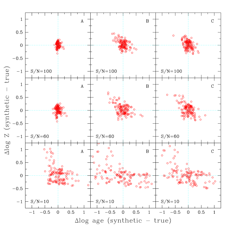
Figure 11: The age-metallicity degeneracy. The x-axis maps the difference between the output and input log age, with the corresponding difference in $\log Z$ plotted along the y-axis. Circles correspond to age and $Z$ computed from the mean (${\bf x},A_{V}$), whereas dots correspond to the best model sampled. All 126 test galaxies are plotted. The different panels correspond to combinations of the data quality ($S/N$, labeled in the bottom-left corners) and the set of observables (top-right) used in the synthesis.

4.4 Metallicity grouped proportions

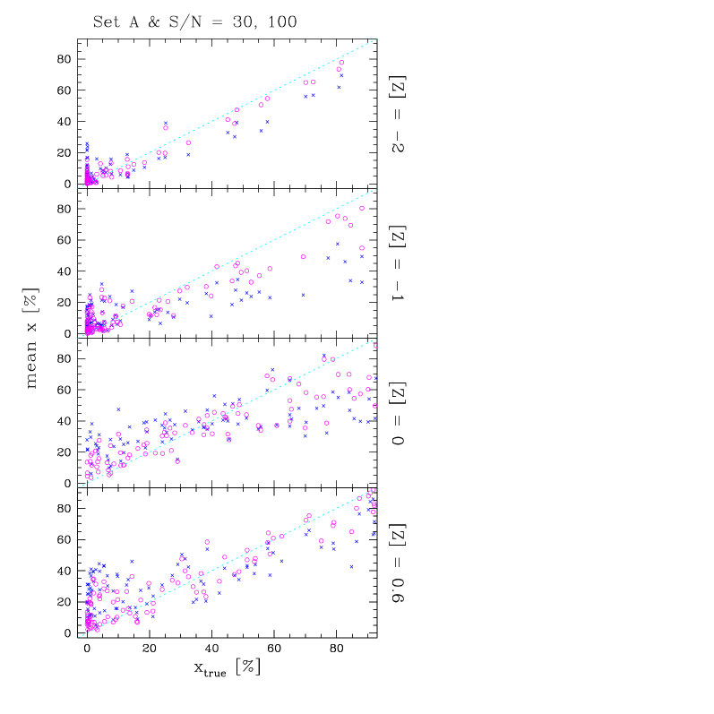
Figure 12: Metallicity binned light fractions in 100 input test galaxies versus the corresponding synthetic means. Circles correspond to $S/N=100$, and crosses to $S/N=30$, both for Set A observables. The ‘resolution power’ of the base is much better for ages (Fig. 9) than for metallicities.

The results for $Z$ binned proportions, plotted in Fig. 12, are not nearly as good as those for the age binned groups. With the exception of the $Z=10^{-2}Z_{\odot}$ bin, which is actually represented by just one element (Table 1), the scatter in the input $\times$ output $Z$-binned proportions is so large for all other $Z$’s that one is forced to conclude that no accurate description of the chemical history of galaxies can be afforded with this spectral base. Given this limited $Z$ ‘resolution power’, one might consider removing intermediate components such as 2, 3 and 6. However, as we concluded that only the age distribution can be assessed with the base, there is no obvious advantage in this further reduction. This situation can be improved by providing a priori constraints on the occupancy of the age-$Z$ plane, like those imposed by B88 based on chemical evolution arguments, since these effectively reduce the dimensionality of the base to typically 8 components, thus alleviating the confusion between components and producing better focused results. The validity of this prior input external to the synthesis process, nonetheless, has to be evaluated in an object by object basis. In this study we followed S91 in not imposing any such extra information, as this approach encompasses a larger class of evolutionary scenarios and thus contemplates more possible applications.

4.5 Best $\times$ Mean Parameters

Throughout these experiments, we have consistently used the mean parameters as an estimate of the result of the synthesis. This convention was deliberately chosen to follow the more widely employed version of EPS with this base and thus to allow a reassessment of previous results. Furthermore, the mean is a convenient and reasonable way to summarize the results insofar as it represents a ‘center of mass’ of acceptable solutions. The severe biases identified in the mean synthetic population vector, however, raise the question of whether alternative approaches should be pursued instead.

By definition, minimization oriented techniques would do a better job at recovering the input parameters. Indeed, we verified that the best model population vector sampled in the Markov chain is much closer to ${\bf x}_{true}$ than its expected value, an agreement which can only be improved given that the Metropolis sampler is not an optimal minimization procedure. Though the simulations confirmed our expectation that for small errors the mean and best solutions should both converge to the true parameters, it was surprising to realize how easily $\overline{\bf x}$ moves away from ${\bf x}_{true}$, and consequently also from ${\bf x}_{best}$. Very small uncertainties in the observables, at the levels of $S/N>300$, are enough to set powerful compensation effects into operation (e.g., Figs. 3 and 4), shifting the components of $\overline{\bf x}$ away from their true values due to the asymmetric redistribution of the probability in ${\bf x}$-space.

Minimization procedures can in principle overcome this bias, as illustrated by the success of the S91 and Pelat (1997) tests as well as by our (not optimized) results for ${\bf x}_{best}$. A further bias in mean solutions is that they always produce $\overline{x_{i}}>0$. Real galaxies, even if synthesizable by the base, are likely to have observables outside synthetic domain due to measurement errors. As shown by Pelat (1997, 1998), the best model in this case lies at the surface of the synthetic domain, where very often several of the ${\bf x}$-components are 0. In these aspects, minimization algorithms are more suitable than the more traditional sampling approach. However, the high susceptibility of the synthesis to the data quality indicates that minor perturbations in the input observables, within their errors, may seriously affect the estimation of the best model parameters. The stability of the best solution is thus likely to be more fragile than that of the mean solution, which takes into account the effects of the errors in the observables in the trade-off between an optimal and a statistically acceptable fit of the data. We have in fact detected this effect in a series of simulations, but a more careful study, with specialized minimization techniques is required to quantify it properly. It would be particularly interesting to carry out this test with the method developed by Pelat (1997) applied to the base used in this work. His Monte Carlo tests with a $n_{\star}=10$ stellar base and $n_{W}=19$ equivalent widths produced essentially unbiased population fractions even for $S/N$ as low as 10. Extending his formalism to synthesize galaxy colors would also be desirable.

In any case, because of the nature of the EPS problem and the structure of Bica’s base, relatively large discrepancies in the parameters do not necessarily translate into large differences in the synthesized quantities. In this respect, the difference between mean and best models is largely academic, as the mean solution already does an excellent job in fitting the observables (Fig. 7).

5 Summary

In this paper we have revisited the method of Empirical Population Synthesis with the aims of improving it both at the formal and computational levels, and exploring its efficacy as a tool to probe the population mixture of galaxies. Our results can be divided into three parts.

(1) A simple probabilistic formulation of the problem was presented, which puts this method, traditionally employed in a less formal way, onto a mathematical footing. It was shown how former applications of the method fit into the probabilistic formulation, thus providing some a posteriori justification for previous results.

(2) An importance sampling scheme, based on the Metropolis algorithm, was developed and tested. It provides a more efficient and smooth mapping of the probability distribution of the parameters than is possible with the commonly used uniform grid sampling.

(3) In the third part of the paper, we applied the formulation and sampling method to a series of test galaxies constructed out the $n_{\star}=12$ star-clusters base of S91. The tests explored the ability to reconstruct the model parameters, which carry a record of the star formation and chemical evolution in galaxies, in the presence of (i) observational errors and (ii) limited data. This study centered on the comparison of input parameters with the mean synthetic solution ($\overline{\bf x},\overline{A_{V}}$), as this is the most common form of EPS in the literature with this base, and a systematic evaluation of the consistency of this method has not been carried out before. The main results of this study can be summarized as follows:

• (a) The allowance for errors in the observables sparkle linear dependences within the base elements. This induces systematic biases in $\overline{\bf x}$, redistributing the probability in components with a large fractional contribution to the integrated spectrum among similar components. This happens preferentially for components of same age. Though this was a predictable result, it was surprising to realize how powerful this effect is. For any realistic $S/N$, the bias is such that in most cases one cannot trust the estimates of all 12 individual components of $\overline{\bf x}$ to any useful level of confidence.

• (b) Reducing the number of observational constraints, due to incomplete coverage of the 3300–9000 Å spectral interval spanned by the base, has the same overall effect as reducing the data quality, that is, to broaden, shift and skew the probability distribution of the $x_{i}$’s. We find that synthesizing colors as well as equivalent widths yields substantially better results than synthesizing $W$’s only. The need to account for the extinction as an extra parameter is largely compensated by the better focused ${\bf x}$ obtained by considering the color information, particularly for populations of 100 Myr and younger. Unlike for the individual population fractions, we do not detect systematic biases in the estimates of $A_{V}$.

• (c) Despite the difficulty to retrieve accurately the detailed population vector, the observables are very precisely reproduced by the mean solution. The mapping between the parameters and observables spaces is thus highly ‘degenerate’. The nature of this ‘non-uniqueness’ is not algebraic, as it happens also when the number of free parameters exceeds the numbers of observables and in undetermined cases where the solution is known to be unique. Instead, it is related to the possibility of mimicking to a statistically indistinguishable level the effects of certain base elements by linear combinations of other elements. This happens even for tiny observational errors, inducing a ‘spill over’ of the likelihood among base components, carrying the mean solution along.

• (d) The structure of the base reflects the fact that evolution is the main source of variance in stellar populations. Accordingly, we found that grouping the $\overline{\bf x}$ components in their five age bins produces much more reliable results, and we recommend this procedure when evaluating the detailed population vector obtained in previously published results with this base. Some confusion between the 1 and 10 Gyr populations also takes place due to the age-$Z$ degeneracy, but this can be minimized with an adequate spectral coverage (measuring all observables in the base) and $S/N\mathrel{\hbox{\raise 2.15277pt\hbox{$>$}\hbox to0.0pt{\hss\lower 2.15277pt\hbox{$\sim$}}}}30$. Grouping the results for the four different $Z$’s in the base is also recommended, but caution must be exerted when interpreting the results since these are much less precise than the age-binned proportions.

The difficulties to retrieve accurately the true stellar population parameters stem from two sources: (i) The convention to represent the results of the synthesis by the mean solution, and (ii) limitations imposed noise-induced linear dependences in the base. Minimization techniques may be instrumental in overcoming the biases in the mean population vector, which ultimately limit the resolution of the 12-D base to its 5 age bins. Within our probabilistic formulation, other priors can be investigated. Maximum Entropy, for example, is a prior that has been applied successfully to inverse problems formally similar to population synthesis, like image restoration. However, more than improvements on the method, which are possible and desirable, further work on the base itself will certainly be needed. Indeed, the limited age and $Z$ ‘resolution power’ of the base employed here lies at the heart of all difficulties identified in this paper. Including other spectral indices, modeling the full spectrum and incorporating other relevant information such as mass to light ratios in the synthesis process are possibles ways to progress in this direction.

References

- [] Bica E., 1988, A&A, 195, 76
- [] Bica E., Alloin D., 1986a, A&A, 162, 21
- [] Bica E., Alloin D., 1986b, A&AS, 66, 171
- [] Bica E., Alloin D., 1987, A&A, 186, 49
- [] Bica E., Alloin D., Schmidt A. A., 1990, A&A, 228, 23
- [] Bica E., Alloin D., Schmitt H. R.,1994, A&A, 283, 805
- [] Bonatto C., Bica E., Alloin D., 1995, A&AS, 112, 71
- [] Boisson C., Joly M., Moultaka J., Pelat D., Serote Roos M., 2000, A&A, 357, 850
- [] Bonatto C., Bica E., Pastoriza M. G., Alloin D., 1996, A&AS, 118, 89
- [] Bonatto C., Pastoriza M. G., Alloin D., Bica E., 1998, A&A, 334, 439
- [] Bonatto C., Bica E., Pastoriza M. G., Alloin D., 1999, A&A, 343, 100
- [] Bonatto C., Bica E., Pastoriza M. G., Alloin D, 2000, A&A, 355, 99
- [] Bruzual G., Charlot S., 1993, ApJ, 405, 538
- [] Charlot S., Bruzual G., 1991, ApJ, 367, 126
- [] Cardelli J. A., Clayton G. C., Mathis, J. S. 1989, ApJ. 345, 245
- [] Cid Fernandes R., Storchi-Bergmann T., Schmitt H. R., 1998, MNRAS, 297,579
- [] De Mello D. F., Keel W. C., Sulentic J. W., Rampazzo R., Bica E., White R. E. III, 1995, A&A, 297, 331
- [] Faber S. M., 1972, A&A, 20, 361F
- [] Fioc M., Rocca-Volmerange B., 1997, A&A, 326, 950
- [] Guiderdoni B., Rocca-Volmerange B., 1987, A&A, 186, 1
- [] Jablonka P., Alloin D., 1995, A&A, 298, 361
- [] Jablonka P., Alloin D., Bica E., 1990, A&A, 235, 22
- [] Joly M., 1974, A&A, 33, 177
- [] Kong X., Cheng F. Z., 1999, A&A, 351, 477
- [] Larson R. B., Tinsley B. M., 1974, ApJ, 192, 293
- [] Larson R. B., Tinsley B. M., 1978, ApJ, 219, 46
- [] Leão J. R. S., 2001, MSc Thesis, Universidade Federal de Santa Catarina
- [] Leitherer C. et al. , 1996, PASP, 108, 996L
- [] Leitherer C., Schaerer D., Goldader, J. D., Delgado, R. M., González R., Carmelle K., Denis F., de Mello D. F.; Devost D., Heckman T. M., 1999, ApJS, 123, 3
- [] MacKay D., 2001, Information Theory, Pattern Recognition and Neural Networks, http://wol.ra.phy.cam.ac.uk/mackay/
- [] Metropolis N., Rosenbluth A., Teller A., Teller E., 1953, J. of Chem. Phys., 21, 1087.
- [] Moultaka J., Pelat D., 2000, MNRAS, 314, 409
- [] O’Connell R. W.,1976, ApJ, 206, 370
- [] O’Connell R. W., 1986, in Stellar Populations, ed. C. Norman, A. Renzini, M. Tosi (Cambridge: Cambridge Univ. Press), p.213
- [] O’Connell R. W., 1994, in Nuclei of Normal Galaxies: Lessons from the Galactic Center, ed. R. Genzel (Dordrecht: Kluwer),
- [] O’Connell R. W., 1996, in From Stars to Galaxies: The impact of stellar physics on galaxy evolution, eds. C. Leitherer, U. Fritze-von-Alvensleben, J. Huchra (ASP: San Francisco),
- [] Pelat D., 1997, MNRAS, 284, 365
- [] Pelat D., 1998, MNRAS, 299, 877
- [] Pickles A. J., 1985, ApJ, 296, 340
- [] Press W. H., Teukolsky S. A., Vetterling W. T., Flannery B. P., 1992, Numerical Recipes, 2nd. edition (Cambridge: Cambridge University Press)
- [] Raimann D., Bica E., Storchi-Bergmann T., Melnick J., Schmitt H. R., 2000, MNRAS, 314, 295
- [] Serote Roos M., Boisson C., Joly M., Ward M., 1998, MNRAS, 301, 1
- [] Serote Roos M., Boisson C., Joly M. 1996, A&A, 117, 93
- [] Schmidt A. A., Copetti M. V. F., Alloin D., Jablonka P., 1991, MNRAS, 249, 766
- [] Schmidt A. A., Bica E., Alloin D., 1990, MNRAS, 243, 620
- [] Schmidt A. A., Bica E., Dottori H. A., 1989, MNRAS, 238, 925
- [] Schmitt H. R., Bica E., Pastoriza, M. G., 1996, MNRAS, 278, 965
- [] Schmitt H. R., Storchi-Bergmann T., Cid Fernandes R., 1999, MNRAS, 303, 173
- [] Silva D., Cornell M., 1992, ApJS, 81, 865
- [] Spinrad H., Taylor B. J., 1971, ApJS, 22, 445
- [] Tinsley B. M., 1972, A&A, 20, 383
- [] Worthey G., 1994, ApJS, 95, 107