Atmospheric Turbulence Measurements with the Palomar Testbed Interferometer

Abstract

Data from the Palomar Testbed Interferometer, with a baseline length of 110 m and an observing wavelength of $2.2\ \mu{\rm m}$, were used to derive information on atmospheric turbulence on 64 nights in 1999. The measured two-aperture variance coherence times at $2.2\ \mu{\rm m}$ ranged from 25 msec to 415 msec (the lower value was set by instrumental limitations—the interferometer could not operate when the coherence time was lower than this). On all nights, the spectrum of the short time scale ($<600$ msec) delay fluctuations had a shallower spectrum than the theoretical Kolmogorov value of 5/3. On most nights, the mean value of the power law slope was between 1.40 and 1.50. Such a sub-Kolmogorov slope will result in the seeing improving as the $\approx 0.4$ power of wavelength, rather than the slower $0.2$ power predicted by Kolmogorov theory.

On four nights, the combination of delay and angle tracking measurements allowed a derivation of the (multiple) wind velocities of the turbulent layers, for a frozen-flow model. The derived wind velocities were all $\leq 4\ {\rm m\ s^{-1}}$, except for a small $10\ {\rm m\ s^{-1}}$ component on one night.

The combination of measured coherence time, turbulence spectral slope, and wind velocity for the turbulent layer(s) allowed a robust solution for the outer scale size (beyond which the fluctuations do not increase). On the four nights with angle tracking data, the outer scale varied from 6 to 54 m, with most values in the 10–25 m range. Such small outer scale values cause some components of visibility and astrometric errors to average down rapidly.

1 Introduction

Optical and near infrared interferometers, by virtue of their long baselines, can achieve angular resolutions better than is possible with a single telescope. However, the atmosphere imposes serious limits on interferometer sensitivity, via the coherence length ($r_{0}$) and coherence time ($t_{0}$): the length and time scale over which atmospheric effects change significantly. At optical and near infrared wavelengths, atmospheric phase variations are dominated by the temperature/density fluctuations of the dry air component.

Conversely, interferometric observations can yield detailed information on atmospheric turbulence on spatial scales larger than those of single apertures. In order to operate, interferometers need to measure (and correct) both delay and angle fluctuations. The time series of these measurements gives temporal and spatial information on atmospheric turbulence. The correlations in delay fluctuations over a finite baseline length can potentially provide additional information.

We used the Palomar Testbed Interferometer (PTI) (Colavita et al., 1999) for atmospheric measurements. PTI has three siderostats (only two of which can be used at one time). It can operate at wavelengths of 1.6 and $2.2\ \mu{\rm m}$, with simultaneous operation possible. All the data reported in this paper were taken on a 110 m baseline (oriented $20^{\circ}$ east of north), at a wavelength of $2.2\ \mu{\rm m}$ (2.0–2.4 $\mu{\rm m}$ passband). Although the interferometer has a dual star mode (for narrow angle astrometry), only data from single star mode was used in this analysis.

There were multiple motivations for this study. The first was to better understand the physics of atmospheric refractivity fluctuations. The second was to quantify the atmospheric error in astronomical measurements (especially those with an interferometer), and perhaps devise improved observational strategies. The third motivation was to look for instrumental error sources, by searching for deviations from an atmospheric signature.

2 Observations and data selection

2.1 Interferometer Delay Data

During PTI operation, the position of the optical delay line, relative to a standard fiducial point, is monitored by laser metrology, recorded at 500 Hz, and averaged in post processing to match the white-light sample time of 10 or 20 msec. The delay line follows a predicted sidereal trajectory. A correction is supplied by the output of the fringe tracker, which adjusts the delay with a 5–10 Hz closed-loop bandwidth to follow the white-light fringe in the presence of atmospheric turbulence and imperfect baseline and astrometric knowledge.

The fringe phase is measured for each 10 or 20 msec sample in a broadband, “white-light” channel, as well as in each of 5 spectral channels across the band. The white-light phase, which has a high SNR per sample, represents the error of the fringe tracker; by adding the white light phase (scaled to delay units) to the measured delay line position, we obtain the total delay at 10 or 20 msec intervals.

The white-light phase measurements are all modulo-$2\pi$ radians; phase unwrapping maintains continuity during tracking, but undetected unwrapping errors can occur due to low SNR or rapid atmospheric motion. These are nominally detected and corrected (one cycle at a time) at a lower rate, of order 1 Hz, using group delay measurement from the phases measured across the 5 spectral channels (Colavita et al., 1999). While the group delay provides an absolute measurement, the low correction rate means that some fraction of the data can be off the central white-light fringe, with the fraction growing for poor seeing. We used four selection criteria to minimize such ‘cycle slips.’ First, sources with fringes weaker than a threshold value were excluded. Second, only scans with an average of $<1.0$ detected fringe lock breaks per 24 s output record were used. This criterion biased our results, by excluding approximately one third of the total data: nights (and segments of nights) with noisy atmospheric conditions. However, it was necessary in order to avoid contamination from instrumental effects. Third, whenever group delay measurements indicated a cycle slip in the fringe tracking, 0.5 s of data at that epoch were flagged and not used in the analysis. Fourth, sources brighter than a threshold value were not used. Fringe data is recorded when locked on the white-light fringe, as ascertained by the fringe signal-to-noise ratio. Bright sources could be tracked on sidelobes of the central fringe with the current implementation of fringe centering.

2.2 Star Tracker Angle Data

During interferometer operations, the angle of each starlight beam was sensed (relative to the optical axis on the beam combiner table) every 10 msec. This “error signal” was used to drive a fast steering mirror, with a closed loop bandwidth of 5 Hz. The fast steering mirror (FSM) position was desaturated into the siderostat positions with a bandwidth of $\approx 0.1$ Hz.

The three component signal complicated the use of the star tracker data for atmospheric measurements. Fortunately, the atmospheric timescales of interest were shorter than the timescale for desaturation of the FSMs. It was not feasible to add the error signal to the FSM positions. With the quad-cell sensor used for angle tracking, the gain is a function of the seeing-dependent spot size. While not an issue for a conservative closed-loop system, this does prevent accurate combination of the error with the mirror position to get angle variations at all frequencies. Therefore, we used the FSM positions by themselves, with separate analysis of the error signals in order to set limits on short timescale angle variations.

We used star tracker data only during periods when fringes were being tracked (i.e. the time gaps in the fringe white light files were used as a flag to edit out similar time periods in the star tracker data).

3 Data Analysis

3.1 Delay Data

3.1.1 Sidereal Fit

The time series of delay (and phase) measurements contained large (tens of meters) geometric components, in addition to atmospheric components. To remove the geometric component, we subtracted a least squares sidereal fit from all the data on a source on a given night:

$$a+b\sin({\rm ST})+c\cos({\rm ST})$$

Here, ST represents sidereal time. By solving for three parameters ($a$, $b$, and $c$), our residuals were insensitive to uncertainties in the length or orientation of the interferometer baseline, or to the zero point in the delay line metrology.

In order to avoid removing significant short term ($<100$ s) atmospheric signature from our data in the fitting process, we only used sources with multiple scans on the same night. The time span for the sidereal fit was therefore always $>1000$ s. Numerical tests showed that a sidereal fit over a duration $T_{\rm fit}$ caused a noticeable suppression in the structure function of the residuals on time scales as short as $T_{\rm fit}/10$, with larger effects on longer timescales.

3.1.2 Structure Functions

Using the residual (i.e. post sidereal fit) delay/phase time series, structure functions $D_{\tau}(\Delta t)$ were calculated:

$$D_{\tau}(\Delta t)\equiv\left<\left[\tau(t+\Delta t)-\tau(t)\right]^{2}\right>$$ (1)

Here $\tau(t)$ is the residual delay at time $t$, and the $<>$ brackets denote ensemble averaging. With observations scheduled for amplitude visibility measurements (the majority of our data), the scan lengths were typically 130 s. One structure function was calculated for each scan. On some nights, long scans (20–30 min.) were made, solely for atmospheric measurements. For those scans, structure functions were calculated for each 3 minute segment of data.

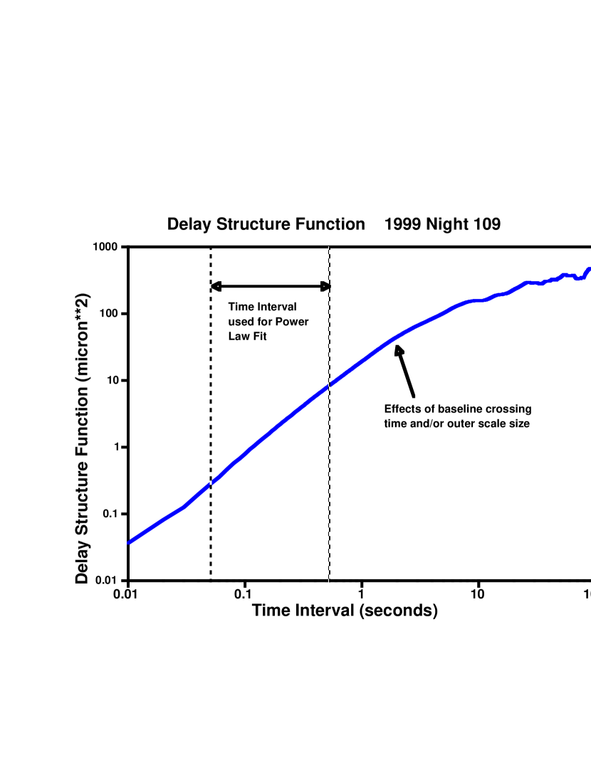
A typical delay structure function is shown in Figure 1. On timescales from 50 msec to $\approx 1$ s, a clean power law slope was seen in the structure function of nearly every ($>90$%) scan. On the shortest timescales ($<50$ msec), the structure function for many scans exhibited power above that extrapolated from the slope at longer (50–500 msec) timescales. We interpret this excess power as being due to instrumental effects (e.g vibrations). On timescales longer than $\approx 1$ s, the slope of $D_{\tau}$ decreased, due to some combination of outer scale length and baseline crossing effects (i.e. the product of wind speed and time interval becomes comparable to or greater than the baseline length). The long baseline (110 m) of PTI, compared to that of other optical/IR interferometers, has a longer wind speed crossing time. There is therefore a relatively long time interval ($>1$ s) over which the fluctuations at the two siderostats are uncorrelated. As discussed later, outer scale effects were more important than the effect of a finite baseline length, at least for the four nights on which we recorded star tracker data from both siderostats, and were able to measure the outer scale length.

Figure 1: Typical delay structure function. The fitted parameters for this scan are a slope of 1.46 and a coherence time of 122 msec.

An alternate method of quantifying fluctuation statistics is power spectral density. Structure functions have the advantage of being unaffected by gaps in the data, and allow a more direct calculation of the dependence of seeing on wavelength, or astrometric precision on baseline length and integration time. The comparison between power spectral density and structure functions is discussed in section 4.3.

3.1.3 Extracting slope and coherence time

A least squares fit to the slope of $D_{\tau}$ was made for each scan, over the interval 50–500 msec (10 msec integration mode) or 60–600 msec (20 msec integration mode). Equal weight was given to each logarithmic time interval in the fit. Results from a given scan were not used if the rms residual to the fit was $>0.02$ in log-log space, or there was too little data (time span $<100$ s or $>40$% of the data from the span missing). Scans with large residuals did not exhibit a simple power law turbulence spectru. As a result, these scans could not be accurately characterized by a single power law index, and we chose not to use them in further analysis.

The two parameters from the fit were the slope and intercept. We wished to derive the coherence time $T_{0,2}$, defined as the time interval over which the interferometer phase fluctuations have a variance of $1\ {\rm radian}^{2}$. Our notation follows that in Colavita et al. (1999); the “2” refers to the contributions from the two apertures of the interferometer.

The variance $\sigma^{2}_{\tau}(T)$ of delay over a time interval $T$ is (Treuhaft & Lanyi, 1987):

$$\sigma^{2}_{\tau}(T)={1\over T^{2}}\int_{0}^{T}(T-\tau)D_{\tau}(t)dt$$ (2)

If $D_{\tau}(\Delta t)=c_{0}(\Delta t)^{\beta}$,

$$\sigma^{2}_{\tau}(T)={c_{0}T^{\beta}\over(1+\beta)(2+\beta)}$$ (3)

If $D_{\tau}(t)$ is expressed in ${\rm radian}^{2}$, we obtain

$$T_{0,2}=\left[{(1+\beta)(2+\beta)\over c_{0}}\right]^{1/\beta}$$ (4)

We can convert from our measured two aperture variance coherence times $(T_{0,2})$ at $2.2\ \mu{\rm m}$ to one aperture difference times $(\tau_{0,1})$ at $0.55\ \mu{\rm m}$, as measured in adaptive-optics applications. Setting $c_{0}\tau_{0,1}^{\beta}=2(0.55/2.2)^{2}$, we get

$$\tau_{0,1\ (0.55\ \mu{\rm m})}=\left[{0.125\over(1+\beta)(2+\beta)}\right]^{1/\beta}T_{0,2\ (2.2\ \mu{\rm m})}$$ (5)

Our data were taken over a range of zenith angles (ZA), up to ${\rm ZA}\approx 40^{\circ}$. The value of $D_{\tau}$ at short time scales for a vertical column of uniform turbulence is expected (on theoretical grounds) to vary linearly with the thickness of the column, suggesting that $D_{\tau}$ will be proportional to $\sec({\rm ZA})$. However, if the wind velocity is not perpendicular to the source azimuth, the dependence will be more gradual.

The extreme range of the variation in $T_{0,2}$ from zenith angle variations will be (see eq.[4]) a factor of $(\sec 40^{\circ})^{1/\beta}$. For the values of $\beta$ measured at PTI ($\beta\approx 1.45$), this will be $\approx 1.2$. As shown in section 4, the range of coherence time was much larger than this, even within one night. Therefore, only a small part of the observed variation in $T_{0,2}$ can be due to the range in observed sky directions. The fitted slope should not depend on zenith angle, based on theoretical grounds. We see no dependence in our data.

3.1.4 Contributions from internal seeing

Light from the siderostats is brought into the optics lab via evacuated beam tubes. Within the optics lab, the delay lines operate in air. A “building within a building” design (Colavita et al., 1999) helps to keep this air still and nearly isothermal. A test of the fluctuations within the optics lab, including the long delay lines, gave a delay structure function 1000 times smaller than those on natural stars (M. Swain, private communication). We conclude that refractivity fluctuations within our instrument gave a negligible contribution to our derived atmospheric parameters.

3.2 Star Tracker Data

3.2.1 Structure Function of Angle Data

The time series of starlight arrival angle measurements $\alpha_{x}(t)$ and $\alpha_{y}(t)$, in directions $x$ and $y$, were used to derive angular structure functions, $D_{\alpha_{x}}\left(\Delta t\right)$ and $D_{\alpha_{y}}(\Delta t)$:

$$D_{\alpha_{x}}(\Delta t)\equiv\left<\left[\alpha_{x}(t+\Delta t)-\alpha_{x}(t)\right]^{2}\right>$$ (6)

Separate structure functions were calculated for the Fast Steering Mirror positions and for the error (i.e. residual) values. Typical FSM angular structure functions are shown in Figure 2. $D_{\alpha_{x}}(\Delta t)$ and $D_{\alpha_{y}}(\Delta t)$ rise rapidly and then flatten out. The upturn at the longest time scales ($>0.3$ s) is due to the desaturation of the FSMs into the siderostats.

Figure 2: Typical measured angular structure function. Data from the North star tracker fast steering mirrors are plotted.

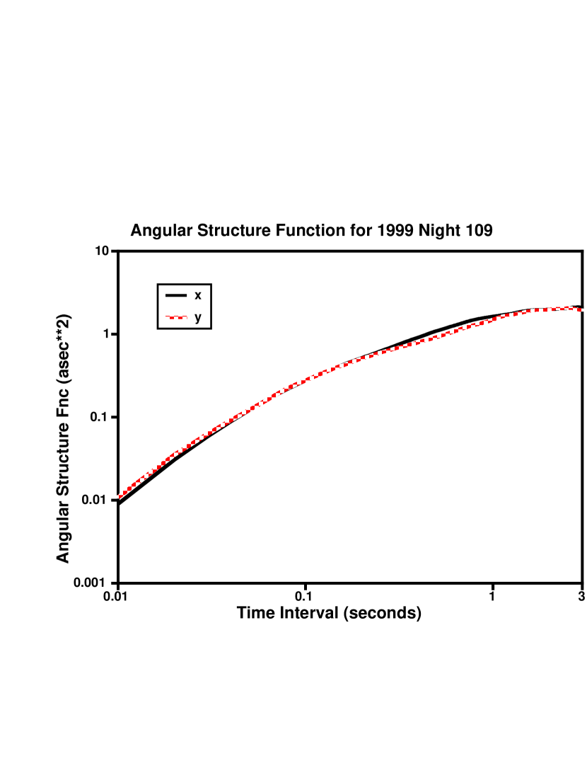
The structure functions for the star tracker error signals showed a sharp rise up to a constant “plateau” for all the scans. This plateau was reached at a time scale of 20–50 msec, depending on the scan. On time scales longer than $\approx 20$ msec (full range 18–25 msec), the structure functions of the FSM positions were larger than the structure functions of the error signals. Therefore, the FSM angular structure functions (e.g. Figure 2) represent all of the actual angle fluctuations, except for a small amplitude, rapid component.

3.2.2 Modeling $D_{\alpha}$

We modeled the measured angles as a least squares fit for the wavefront slope across our apertures, in two ($x$ and $y$) directions (Sarazin & Roddier, 1990). For the $x$-axis slope, we want to minimize

$$S\equiv\int_{0}^{2\pi}d\phi\int_{0}^{R}r\left[\tau(r,\phi,t)-c_{0}-x\alpha_{x}(t)\right]^{2}dr$$

Here $R$ is the radius (20 cm) of our aperture, and $\tau(r,\phi,t)$ is the delay at position $(r,\phi)$ and time $t$ on the aperture. Setting $\partial S/\partial\alpha_{x}(t)=0$, we obtain

$$\alpha_{x}(t)={4\over\pi R^{4}}\int_{0}^{2\pi}\cos\phi d\phi\int_{0}^{R}r^{2}\tau(r,\phi,t)dr$$ (7)

The definition of $D_{\alpha_{x}}(\Delta t)$ gives

$$D_{\alpha_{x}}(\Delta t)=2\left<\alpha_{x}^{2}(t)\right>-2\left<\alpha_{x}(t+\Delta t)\alpha_{x}(t)\right>$$ (8)

Equation(7) leads to:

$$\left<\alpha_{x}^{2}(t)\right>={16\over\pi^{2}R^{8}}\int_{0}^{2\pi}\cos\phi d\phi\int_{0}^{2\pi}\cos\phi^{\prime}d\phi^{\prime}\int_{0}^{R}r^{2}dr\int_{0}^{R}r^{\prime 2}\left<\tau(r,\phi,t)\tau(r^{\prime},\phi^{\prime},t)\right>dr^{\prime}$$ (9)

The analog to equation(8) for the spatial delay structure function $D_{\tau}(\Delta\vec{x})$ is:

$$D_{\tau}(\Delta\vec{x})=2\left<\tau^{2}(\vec{x})\right>-2\left<\tau(\vec{x}+\Delta\vec{x})\tau(\vec{x})\right>$$ (10)

$\left<\tau^{2}(\vec{x},t)\right>$ is assumed to be independent of $\vec{x}$ and $t$, so that this term integrates to zero.

$$\left<\alpha_{x}^{2}(t)\right>=-{8\over\pi^{2}R^{8}}\int_{0}^{2\pi}\cos\phi d\phi\int_{0}^{2\pi}\cos\phi^{\prime}d\phi^{\prime}\int_{0}^{R}r^{2}dr\int_{0}^{R}r^{\prime 2}D_{\tau}(|(r,\phi,t)-(r^{\prime},\phi^{\prime},t)|)dr^{\prime}$$ (11)

With a similar derivation for $\left<\alpha_{x}(t+\Delta t)\alpha_{x}(t)\right>$, we get

$$D_{\alpha_{x}}(\Delta t)={16\over\pi^{2}R^{8}}\int_{0}^{2\pi}\cos\phi d\phi\int_{0}^{2\pi}\cos\phi^{\prime}d\phi^{\prime}\int_{0}^{R}r^{2}dr\int_{0}^{R}r^{\prime 2}\left[D_{\tau}(B)-D_{\tau}(A)\right]dr^{\prime}$$ (12)

$$A\equiv |(r,\phi,t)-(r^{\prime},\phi^{\prime},t)|$$

$$B\equiv |(r,\phi,t+\Delta t)-(r^{\prime},\phi^{\prime},t)|$$

We relate the spatial and temporal structure of the turbulence field with the frozen flow (Taylor) approximation. For sky directions near zenith (as in our observations), the dependence of model $D_{\alpha_{x}}(\Delta t)$ and $D_{\alpha_{y}}(\Delta t)$ values on wind azimuth is relatively minor: $\pm 20$% in amplitude and the timescale of the slope break, compared to the values for a $45^{\circ}$ azimuth. We therefore used an azimuth of $45^{\circ}$ in the calculations. The close agreement between the measured $D_{\alpha_{x}}(\Delta t)$ and $D_{\alpha_{y}}(\Delta t)$ curves suggests that the true wind azimuth was not near $0^{\circ}$ or $90^{\circ}$ (or, more likely, that there was a mix of wind azimuths in the turbulent region of the atmosphere).

3.2.3 Fitting for the wind velocity of the turbulent layers

Once $D_{\tau}(\Delta t)$ is specified, the only free parameter in modeling $D_{\alpha_{x}}(\Delta t)$ is the wind velocity, needed to relate the coherence time ($T_{0,2}$) to the coherence length ($r_{0}$), and $D_{\tau}(\Delta t)$ to $D_{\tau}(\Delta\vec{x})$. For a wind velocity of $v_{w}$ in azimuth $\phi_{w}$,

$$A= \sqrt{(r\cos\phi-r^{\prime}\cos\phi^{\prime})^{2}+(r\sin\phi-r^{\prime}\sin\phi^{\prime})^{2}}$$

$$B= \sqrt{(r\cos\phi+v_{w}\Delta t\cos\phi_{w}-r^{\prime}\cos\phi^{\prime})^{2}+(r\sin\phi+v_{w}\Delta t\sin\phi_{w}-r^{\prime}\sin\phi^{\prime})^{2}}$$

A grid of model wind velocities was used to test the agreement between theoretical and measured angular structure functions. In general, the agreement for a single turbulent flow velocity was poor — the slope change in the model was sharper than in the data. Therefore, models with multiple layers (bulk wind velocities) were used. The turbulence fields in different layers were assumed to be independent, so that their contributions to the angular and delay structure functions could be added. Figures 3 and 4 show the agreement between data and model for single and double layer models, for a scan on 1999, Night 109. Adding even more layers to our models would have resulted in slightly better matches to the shapes of the measured structure functions than in Figure 4. However, it would not have changed the overall scaling mismatch.

There was not enough information in the angular structure functions to closely constrain the velocity of each component, but the general shape of the overall velocity distribution was determined.

Figure 3: Angular structure function from 1999 Night 109 with a single layer ($2.5\ {\rm m\ s^{-1}}$ wind velocity) model. The fit is poor on time scales $>0.2$ s. The overall scaling mismatch is consistent with the amplitude calibration uncertainty of the star tracker.

Figure 4: Angular structure function from the same scan as in Figure 3, with a multiple layer (1 and $4\ {\rm m\ s^{-1}}$ wind velocities) model. The discrepancy between the data and the model on time scales $>0.5$ s is due to desaturation of the fast steering mirrors into the siderostats. The overall scaling mismatch is consistent with the amplitude calibration uncertainty of the star trackers.

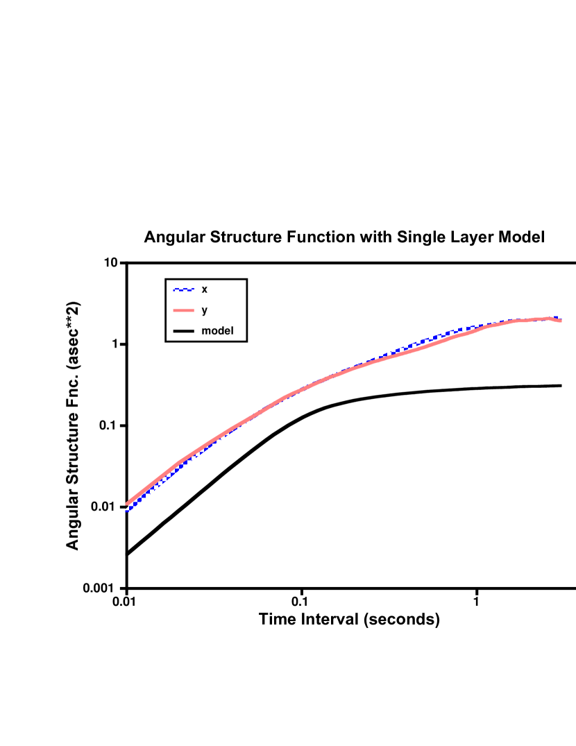
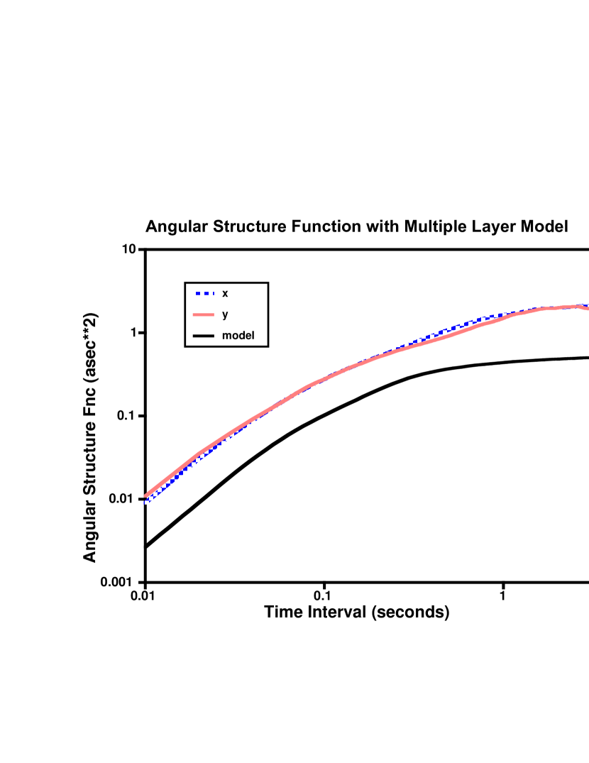
The overall amplitude scale for the FSM angles is uncertain by at least 20%, enough to account for the discrepancy between data and model seen in Figures 3 and 4 (note that the structure function is proportional to the square of the angles). In addition, the model values reflect the average of the conditions at the two siderostats.

4 Results

4.1 Delay Data

Delay data (which passed the selection criteria described above) were obtained for 64 nights in 1999. Table 1 gives a summary of the data volume: number of scans and total time span for each night, along with the mean values of the slope ($\beta$) and coherence time ($T_{0,2}$). For long scans, each 3 minute segment has been counted in the total in Table 1.

Figure 5 shows the mean fitted spectral slopes for the nights with $\geq 10$ usable scans. The vertical bars represent the $1\sigma$ scatter about the mean for that night. The three dimensional Kolmogorov value of 5/3 is shown for comparison.

Figure 5: Mean value of spectral slope ($\beta$) for each night in 1999 with 10 or more scans. The error bars represent the $1\sigma$ scatter about the mean value for that night.

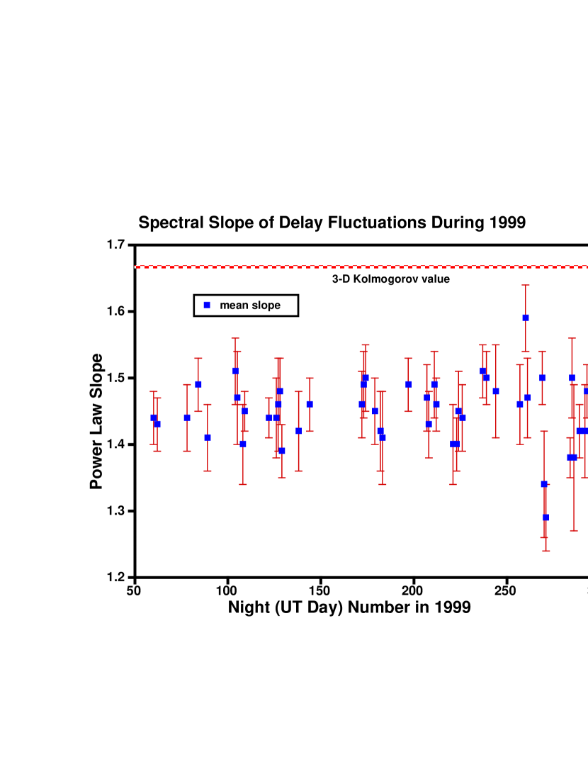
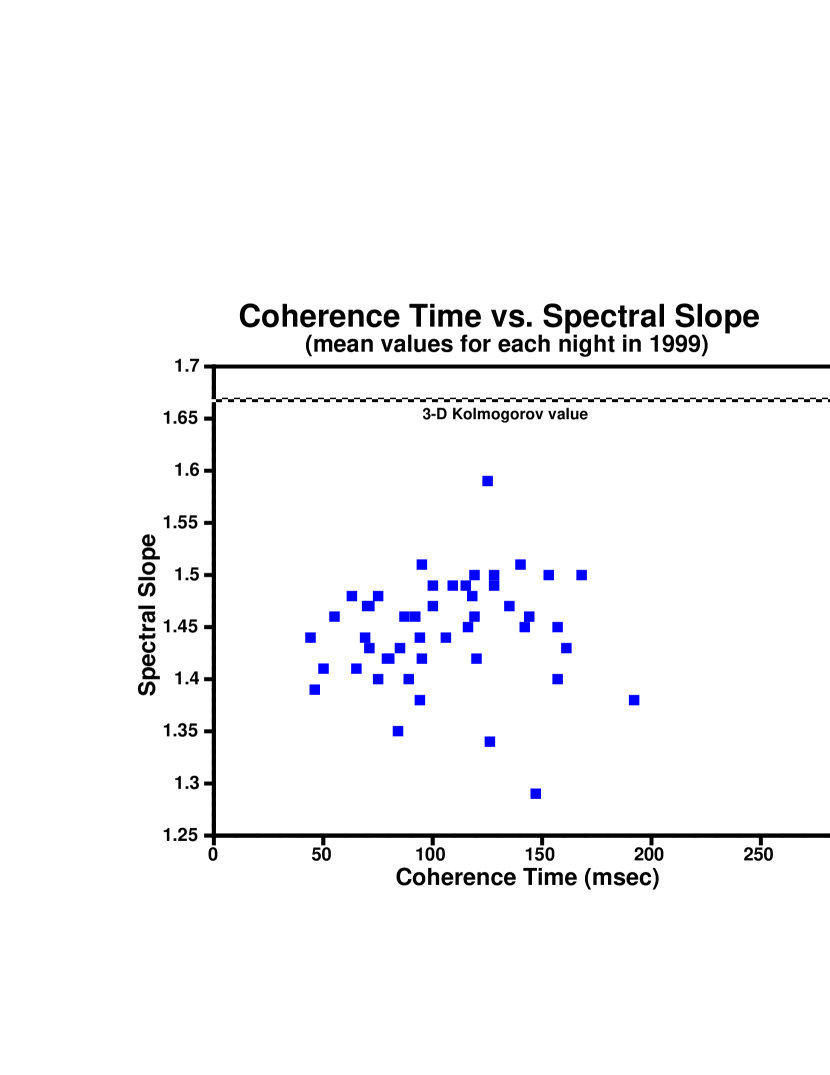
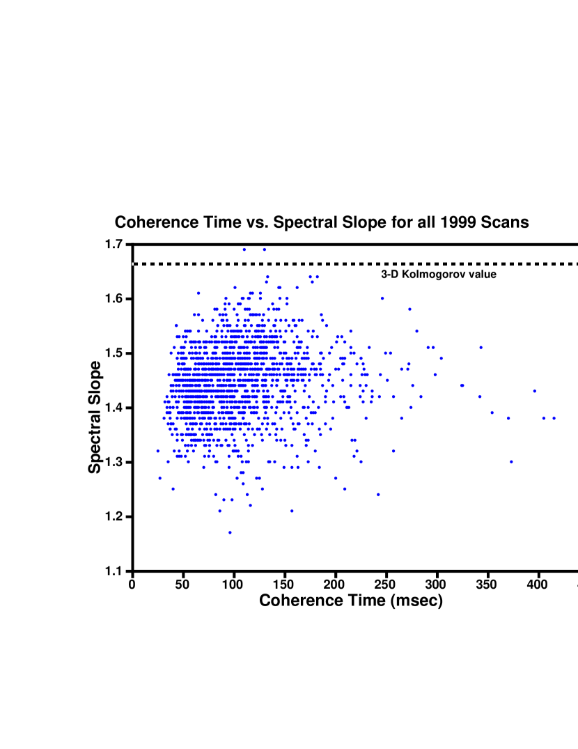
Figure 6 is a scatter plot of the mean slope and coherence time for each night with $\geq 10$ usable scans. Figure 7 is a similar plot for all the data, with one point per scan. There appears to be no obvious correlation between the slope and coherence time. The lower cutoff at $T_{0,2}\approx 30$ msec is a selection effect: for shorter coherence times, there were too many losses of lock to meet our selection criteria (or the atmosphere was too noisy for the interferometer to operate at all).

Figure 6: Scatter plot of mean spectral slope against mean coherence time for each night in 1999 with 10 or more scans.

Figure 7: Scatter plot of mean spectral slope against mean coherence time for each scan in 1999. The apparent quatization is due to the precision of 0.01 used in saving values of the fitted slope.

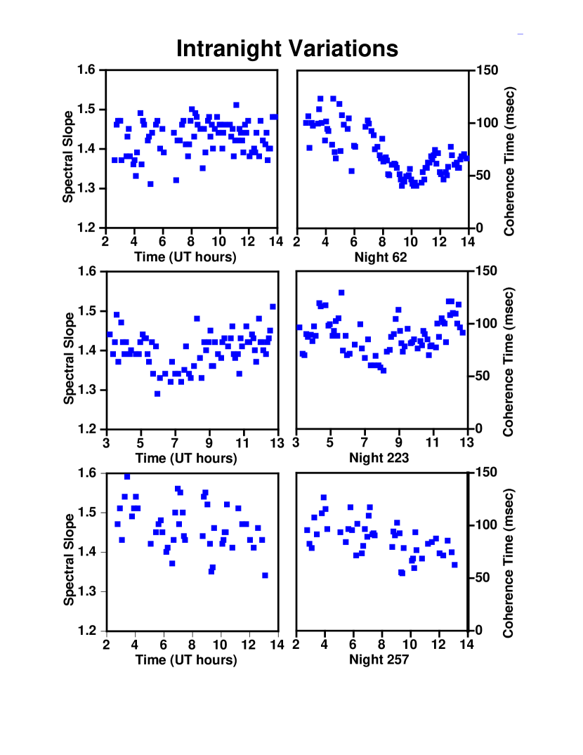
The variations in $\beta$ and $T_{0,2}$ within individual nights did not fit into any obvious pattern. Figure 8 shows the variations for nights 62, 223, and 257 in 1999 (this includes the two nights with the largest number of scans, and the two nights with the largest time spans). For most nights, there was no obvious trend in $\beta$ with time. The coherence time varied by factors of 2–4, sometimes on timescales of $<1$ hr (e.g. on Night 62). This result is consistent with reports of variations in seeing on similar time scales (e.g. Martin et al. 1998).

An exponent of $\beta$ in the delay structure function corresponds to an exponent of $-(1+\beta)$ in the one-dimensional spectrum of delay fluctuations (Armstrong & Sramek 1982). For a Kolmogorov spectrum, the power spectrum exponent is $-8/3$.

Figure 8: Time history of spectral slope and coherence time during 1999 Nights 62, 223, and 257.

4.2 Angle Tracking Data

There were only four nights with extensive data recorded from both North and South star trackers. Table 2 gives the results of the velocity fitting for those nights. The time variations in the weights of the fitted wind velocities were small ($\sim 10$%) within each night.

The weights in Table 2 represent the relative contributions to the coherence time (i.e. delay variations). To get the contribution of component $i$ to the coherence length, these weights should be scaled by $v_{i}^{-\beta}$, where $v_{i}$ is the velocity of component $i$ and $\beta$ is the measured slope of the delay structure function (see Table 1). Therefore, the contributions of low velocity ($\sim 1\ {\rm m\ s^{-1}}$) turbulent flow to $r_{0}$ are more dominant than suggested by the weights in Table 2.

4.3 Long Time Intervals/Outer Scale Lengths

If we assume that delay variations are due to a turbulence field convected past the telescopes (frozen flow), variations in $T_{0,2}$ could be due either to variations in the flow velocity or to variations in the properties of the turbulence field. Variations in the measured flow velocity (described above) within individual nights were small. Therefore, variations in $T_{0,2}$ must primarily reflect variations in the turbulence field. As a measure of the total fluctuation amplitude, we used $D_{\tau}(50\ {\rm s})$: the delay structure function at a time interval of 50 s. This interval is approximately half the length of our shortest scans, and is therefore approximately the longest interval over which we can get good statistics for $D_{\tau}$ in one scan. By an interval of 50 s, $D_{\tau}$ had nearly leveled off for most scans.

For those scans (on nights 109, 211, 212, and 271) with star tracker data, we can use $D_{\tau}(50\ {\rm s})$ to solve for an outer scale size of the turbulence. For $D_{\tau}(\Delta t)=c_{0}(\Delta t)^{\beta}$ and a set of velocities $v_{i}$ with weights (fractional contribution to $D_{\tau}$) $f_{i}$, the structure function will saturate at a value:

$$D_{\tau}({\rm max})=c_{0}\sum_{i}\left[f_{i}\left({L_{0}\over v_{i}}\right)^{\beta}\right]$$ (13)

Here $L_{0}$ is the structure function definition of the outer scale length: the spatial delay structure function $D_{\tau}(d)$ reaches a maximum value of $c_{0}L_{0}^{\beta}$. The derived outer scale values, for each scan with dual (north and south) angle tracking data, are shown in Figure 9.

Figure 9: Outer scale length vs. time for the four nights with star tracker data from both siderostats.

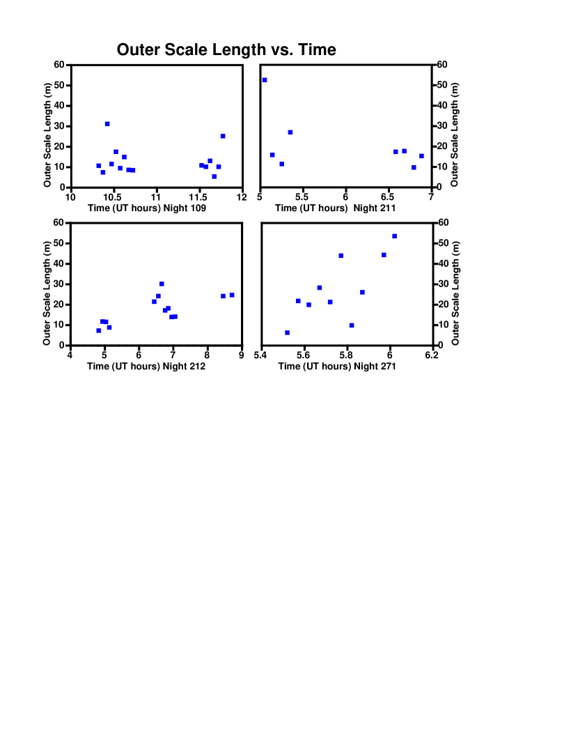
The decision to record dual star tracker data on these four nights was not based on the level of measured turbulence. We therefore expect the results shown in Figure 9 to be representative of the conditions during the full set of 64 nights listed in Table 1. However, these results may not apply to the nights where the coherence time was too short for us to extract atmospheric parameters. We have no constraints on the outer scale length for those ‘noisy’ nights.

An outer scale length in the refractivity power spectral density is generally represented with the von Karman model (Ishimaru 1978):

$$\Phi_{N}(\kappa)\propto\left[\kappa^{2}+\left({1\over{\cal L}_{0}}\right)^{2}\right]^{-11/6}$$ (14)

The spatial frequency $\kappa=2\pi/\lambda$, with $\lambda$ the wavelength of the fluctuation. For the generalization to non-Kolmogorov slopes, the exponent is $-(1+\beta/2)$.

In order to obtain the correspondence between the power spectral density outer scale ${\cal L}_{0}({\rm PSD})$ and the structure function outer scale $L_{0}(D_{\tau})$, equation(14) was first transformed to a refractivity structure function. This refractivity structure function was then numerically integrated to yield a delay structure function. The results on the outer scale correspondence, for three representative values of $\beta$, are:

$$L_{0}(D_{\tau})= 0.94{\cal L}_{0}({\rm PSD})\quad(\beta=5/3)$$

$$= 1.03{\cal L}_{0}({\rm PSD})\quad(\beta=1.50)$$ (15)

$$= 1.18{\cal L}_{0}({\rm PSD})\quad(\beta=1.35)$$

5 Discussion

5.1 Spectral Slope

Our measured power law slopes for short time scale delay variations were largely in the range 1.40–1.50, and were in all cases shallower than the three-dimensional Kolmogorov value of 5/3. The spectral slope was not correlated with the coherence time, at least when atmospheric conditions were stable enough for operation of the interferometer.

The Kolmogorov spectrum is based on dimensional considerations (Tatarski, 1961). Measurements of strong turbulence in a variety of fluids have shown good agreement to Kolmogorov spectra (Grant et al., 1962; Frish & Orszag, 1990). However, atmospheric conditions during astronomical observations involve much weaker turbulence. Intermittent turbulence (Frish et al., 1978) may decrease the slope of the spectrum under these conditions.

Buscher et al. (1995) analyzed atmospheric fluctuations with interferometric measurements from Mt. Wilson, on baselines from 3 to 31 m in length. Based on power spectral densities, they found a mean slope slightly shallower than Kolmogorov, by 0.12 (equivalent to a slope of 1.55 for delay structure functions). Bester et al. (1992) also used data from Mt. Wilson. However, all their short time scale measurements were made with a laser distance interferometer, over a horizontal path of length $\sim 10$ m, located 3 m above the ground. They measured spectral slopes shallower than the Kolmogorov value by nearly 0.30 (i.e. a structure function exponent of $\beta\approx 1.40$).

Our results agree with those of Bester et al. (1992), although our data were taken on approximately vertical line-of-sight paths through the entire atmosphere, and theirs on much shorter paths near the ground. Our results disagree with those of Buscher et al. (1995), if we use the standard correspondence between the exponents of the power spectral density ($\gamma$) and structure function ($\beta$): $-\beta-1\leftrightarrow\gamma$ (Armstrong & Sramek, 1982). However, Bester et al. (1992) report the surprising result that their value of $\gamma$ is often 0.1 or 0.2 steeper than $-\beta-1$ for the same data (their actual comparison is between power spectral density and Allan variance, whose slope is nearly equal to that of the structure function at short time scales). They speculate that the discrepancy may result from occasional bursts with $\beta>2$, for which the $-\beta-1\leftrightarrow\gamma$ connection does not hold.

For $D_{\tau}\propto(\Delta t)^{\beta}$, the dependence of coherence length $r_{0}$ upon wavelength $\lambda$ will be $r_{0}\propto\lambda^{2/\beta}$, and the seeing $(\theta)$ will vary as $\theta\propto\lambda^{1-2/\beta}$. A value of $\beta=5/3$ gives $\theta\propto\lambda^{-0.2}$, while $\beta=1.40$ gives $\theta\propto\lambda^{-0.43}$. Numerous reports of exceptional seeing at infrared wavelengths (e.g. diffraction rings in images with the Palomar 5 m telescope at wavelengths of $10\ \mu{\rm m}$ and even $5\ \mu{\rm m}$) are most easily explained with a steep dependence of seeing vs. wavelength.

For astrometry with ground-based interferometry, a low value of $\beta$ has favorable consequences. Over a baseline of length $B$, the instantaneous delay uncertainty $\Delta\tau_{\rm atm}$ of the atmosphere will be:

$$\Delta\tau_{\rm atm}\sim{\lambda\over 2\pi}\left({B\over r_{0}}\right)^{\beta/2}$$

Here $r_{0}$ is the coherence length at wavelength $\lambda$, and an infinite outer scale length is assumed. For a finite outer scale length $L_{0}$, the baseline length $B$ should be replaced with $L_{0}$.

5.2 Turbulence speed and height

Our derived wind velocity for the turbulent layer(s) (section 4.2) was low: 1–4$\ {\rm m\ s^{-1}}$ (plus a small $10\ {\rm m\ s^{-1}}$ component on one night). For interferometric measurements on only one star at a time, we have no direct constraint on the height of the turbulence. However, the very low velocities suggest that the turbulence was at low altitudes, perhaps even within 100 m of the surface. Treuhaft et al. (1995) derived a low altitude ($<45$ m) for the majority of the turbulence seen at the Mt. Wilson Infrared Spatial Interferometer, based on a correlation between fluctuations seen with the starlight interferometer and a laser distance interferometer.

Simultaneous observations of two (or more) stars with the same pair of siderostats would allow a direct determination of turbulent height.

5.3 Outer Scale Lengths

Our measured outer scale lengths are mostly in the range 10–25 m, in agreement with results reported by others (Coulman et al., 1988; Ziad et al., 1994). All our values are less than half the 110 m length of our baseline, giving us confidence that our results are not significantly corrupted by the finite length of the baseline. Because these outer scale values are based on simultaneous measured delay and angle time series on a long baseline, they are less sensitive to modeling assumptions than most previously published results. Shao & Colavita (1992) derived the effect of a finite outer scale size on the accuracy of narrow angle astrometry. For $L_{0}<<B$ ($B$ is the baseline length), the accuracy improvement over an infinite outer scale, for $\beta=5/3$, is $(L_{0}/B)^{1/3}$. For $L_{0}\approx 15$ m and $B=110$ m, this factor is $\approx 0.5$. For longer baselines, the accuracy improves as $B^{-1}$, rather than as $B^{-2/3}$ for an infinite outer scale.

Table 1: Summary of Atmospheric Data From 1999.

Night	No. Scans	Time Span	Mean $\beta$	Mean $T_{0,2}$
59	6	3.5 hr	1.44	117 msec
60	67	9.8 hr	1.44	69 msec
62	87	11.3 hr	1.43	71 msec
78	48	9.7 hr	1.44	106 msec
84	17	2.9 hr	1.49	100 msec
89	22	6.5 hr	1.41	50 msec
101	7	2.9 hr	1.34	53 msec
104	26	8.6 hr	1.51	95 msec
105	32	9.5 hr	1.47	70 msec
106	7	0.8 hr	1.45	58 msec
108	22	5.4 hr	1.40	157 msec
109	32	5.9 hr	1.45	116 msec
122	12	1.4 hr	1.44	44 msec
126	21	3.4 hr	1.44	291 msec
127	43	5.3 hr	1.46	144 msec
128	34	6.8 hr	1.48	75 msec
129	32	7.1 hr	1.39	46 msec
138	18	5.3 hr	1.42	120 msec
141	6	1.3 hr	1.44	52 msec
144	12	4.9 hr	1.46	55 msec
145	4	1.0 hr	1.44	40 msec
172	24	7.8 hr	1.46	92 msec
173	47	4.4 hr	1.49	128 msec
174	41	4.5 hr	1.50	168 msec
175	9	2.8 hr	1.39	130 msec
177	8	3.2 hr	1.37	56 msec
178	16	7.8 hr	1.43	85 msec
179	32	7.9 hr	1.45	142 msec
180	9	2.2 hr	1.45	227 msec
181	7	0.7 hr	1.40	94 msec
182	12	5.7 hr	1.42	95 msec
183	11	2.7 hr	1.41	65 msec
197	15	4.0 hr	1.49	115 msec
205	5	1.3 hr	1.51	93 msec
207	29	7.4 hr	1.47	135 msec
208	46	8.3 hr	1.43	161 msec
211	41	7.2 hr	1.49	109 msec
212	23	4.8 hr	1.46	119 msec
214	4	0.5 hr	1.41	85 msec
221	31	7.1 hr	1.40	75 msec
223	74	9.5 hr	1.40	89 msec
224	19	5.0 hr	1.45	157 msec
226	34	5.3 hr	1.44	94 msec
231	9	7.5 hr	1.50	151 msec
237	23	5.4 hr	1.51	140 msec
239	27	8.2 hr	1.50	119 msec
244	21	4.9 hr	1.48	118 msec
257	47	10.3 hr	1.46	87 msec
258	6	6.2 hr	1.44	134 msec
260	25	5.1 hr	1.59	125 msec
261	36	9.3 hr	1.47	71 msec
269	40	6.8 hr	1.50	128 msec
270	43	5.2 hr	1.34	126 msec
271	16	3.1 hr	1.29	147 msec
284	13	7.5 hr	1.38	94 msec
285	13	8.0 hr	1.50	153 msec
286	13	5.8 hr	1.38	192 msec
289	23	8.3 hr	1.42	79 msec
292	28	7.9 hr	1.42	80 msec
293	32	10.1 hr	1.48	63 msec
294	5	3.5 hr	1.52	92 msec
297	17	5.5 hr	1.35	84 msec
298	19	5.0 hr	1.47	100 msec

Note. — The five columns are: 1) UT Day number corresponding to a night of observations, 2) Number of usable scans for that night, 3) Time spanned by the scans on that night, 4) Mean spectral slope $(\beta)$ of the scans on that night, and 5) Mean coherence time $(T_{0,2})$ for the scans on that night.

Table 2: Best Fit Turbulent Flow Velocities.

Night	Time Span	Vel. 1	Weight (N)	Weight (S)	Vel. 2	Weight (N)	Weight (S)
109	1.5 hr	$1\ {\rm m\ s^{-1}}$	0.34	0.42	$4\ {\rm m\ s^{-1}}$	0.66	0.58
211	1.8 hr	$0.8\ {\rm m\ s^{-1}}$	0.14	0.16	$3\ {\rm m\ s^{-1}}$	0.86	0.84
212	3.9 hr	$0.5\ {\rm m\ s^{-1}}$	0.09	0.10	$2\ {\rm m\ s^{-1}}$	0.63	0.80
271	0.4 hr	$1\ {\rm m\ s^{-1}}$	0.50	0.57	$4\ {\rm m\ s^{-1}}$	0.50	0.43

Note. — The eight columns are: 1) UT Day number corresponding to a night of observations, 2) Time spanned by the scans with star tracker data on that night, 3) Velocity of component one, 4) Weight of component one for the North siderostat, 5) Weight of component one for the South siderostat, 6) Velocity of component two, 7) Weight of component two for the North siderostat, 8) Weight of component two for the South siderostat.

References

- Armstrong & Sramek (1982) Armstrong, J. W., and Sramek, R. A., 1982, Radio Sci., 17, 1579.
- Bester et al. (1992) Bester, M., Danchi, W. C., Degiacomi, C. G., Greenhill, L. J., and Townes, C. H. 1992, ApJ, 392, 357.
- Buscher et al. (1995) Buscher, D. F. et al. 1995, Appl. Opt., 34, 1081.
- Colvita et al. (1987) Colavita, M. M., Shao, M., and Staelin, D. H. 1987, Appl. Opt., 26, 4106.
- Colavita et al. (1999) Colavita, M. M. et al. 1999, ApJ, 510, 505.
- Coulman et al. (1988) Coulman, C. E., Vernin, J., Coqueugniot, Y., and Caccia, J. L. 1988, Appl. Opt., 27, 155.
- Frish & Orszag (1990) Frish, U., and Orszag, S. A 1990, Physics Today. 43, 24.
- Frish et al. (1978) Frish, U., Sulem, P.-L., and Nelkin, M. 1978, Journal of Fluid Mechanics, 87, 719.
- Grant et al. (1962) Grant, H. L., Stewart, R. W., and Moilliet, A., 1962, Journal of Fluid Mechanics, 12, 241.
- Ishimaru (1978) Ishimaru, A., Wave Propagation and Scattering in Random Media, vol. 2, New York: Academic Press (1978).
- Martin et al. (1998) Martin, F. et al., 1998, A&A, 336, L49.
- Sarazin & Roddier (1990) Sarazin, M., and Roddier, F. 1990, A&A, 227, 294.
- Shao & Colavita (1992) Shao, M., and Colavita, M. M. 1992, A&A, 262, 353.
- Tatarski (1961) Tatarski, V. I., Wave Propagation in a Turbulent Medium, New York: McGraw-Hill (1961).
- Treuhaft & Lanyi (1987) Treuhaft, R. N., and Lanyi, G. E. 1987, Radio Sci., 22, 251.
- Treuhaft et al. (1995) Treuhaft, R. N., Lowe, S. T., Bester, M., Danchi, W. C., and Townes, C. H. 1995, ApJ, 453, 522.
- Ziad et al. (1994) Ziad, A., Borgnino, J., Martin, F., and Agabi, A. 1994, A&A, 282, 1021.