High-Resolution X-ray Spectroscopy and Modeling of the Absorbing and Emitting Outflow in NGC 3783

Abstract

The high-resolution X-ray spectrum of NGC 3783 shows several dozen absorption lines and a few emission lines from the H-like and He-like ions of O, Ne, Mg, Si, and S as well as from Fe XVII–Fe XXIII L-shell transitions. We have reanalyzed the Chandra HETGS spectrum using better flux and wavelength calibrations along with more robust methods. Combining several lines from each element, we clearly demonstrate the existence of the absorption lines and determine they are blueshifted relative to the systemic velocity by $-610\pm 130$ km s^-1. We find the Ne absorption lines in the High Energy Grating spectrum to be resolved with ${\rm FWHM}=840^{+490}_{-360}$ km s^-1; no other lines are resolved. The emission lines are consistent with being at the systemic velocity. We have used regions in the spectrum where no lines are expected to determine the X-ray continuum, and we model the absorption and emission lines using photoionized-plasma calculations. The model consists of two absorption components, with different covering factors, which have an order of magnitude difference in their ionization parameters. The two components are spherically outflowing from the AGN and thus contribute to both the absorption and the emission via P Cygni profiles. The model also clearly requires O VII and O VIII absorption edges. The low-ionization component of our model can plausibly produce UV absorption lines with equivalent widths consistent with those observed from NGC 3783. However, we note that this result is highly sensitive to the unobservable UV-to-X-ray continuum, and the available UV and X-ray observations cannot firmly establish the relationship between the UV and X-ray absorbers. We find good agreement between the Chandra spectrum and simultaneous ASCA and RXTE observations. The 1 keV deficit previously found when modeling ASCA data probably arises from iron L-shell absorption lines not included in previous models. We also set an upper limit on the FWHM of the narrow Fe K$\alpha$ emission line of 3250 km s^-1. This is consistent with this line originating outside the broad line region, possibly from a torus.

1 Introduction

Active Galactic Nuclei (AGNs) often show evidence for deep absorption features from 0.7–1.5 keV which have been typically attributed to O VII (739 eV) and O VIII (871 eV) edges. The ionized gas component creating these features is usually referred to as a ‘warm absorber’ and is seen in many Seyfert 1 galaxies (e.g., Reynolds 1997; George et al. 1998b) and some quasars (e.g., Halpern 1984; Brandt et al. 1997). The fact that these absorption features are seen in $\gtrsim$70% of Seyfert 1s implies that the ionized gas covers a substantial fraction of the central X-ray source. The radial location of the warm absorber is still not well constrained. Several Seyfert 1s have shown warm absorber edge variability on timescales of hours to weeks (e.g., Fabian et al. 1994; Otani et al. 1996; George et al. 1998a, 1998b), suggesting that they have some ionized gas lying at distances characteristic of the Broad Line Region (BLR). Warm absorbers are also a subject of intense theoretical investigation (e.g., Netzer 1993, 1996; Krolik & Kriss 1995; Reynolds & Fabian 1995; Nicastro, Fiore, & Matt 1999). They are expected to be emitters of X-ray lines such as O VII (568 eV), O VIII (653 eV), and Ne IX (915 eV). They are also expected to produce X-ray absorption lines with significant equivalent widths (EWs).

Table 1: Observation Log of NGC 3783

Observatory	Sequence Number	UT start	UT end	Time
(1)	(2)	(3)	(4)	(5)
Chandra	70004500	2000 Jan 20, 23:33	2000 Jan 21, 16:20	56.0
ASCA	77034000	2000 Jan 12, 06:23	2000 Jan 12, 21:21	15.6
ASCA	77034010	2000 Jan 16, 21:00	2000 Jan 17, 13:05	17.6
ASCA	77034020	2000 Jan 21, 04:02	2000 Jan 21, 18:27	04.1
RXTE	30227000	2000 Jan 21, 04:37	2000 Jan 21, 16:56	19.6

^aSum of good time intervals in units of ks. For ASCA the time is the mean from the four detectors.

The bright Seyfert 1 galaxy NGC 3783 ($V\approx 13.5$ mag) has one of the strongest warm absorbers known. Its X-ray spectrum and ionized absorption have been modeled using data from ROSAT (Turner et al. 1993) and ASCA (e.g., George et al. 1998a). The 2–10 keV spectrum is fit by a power law with photon index $\Gamma\approx 1.7$–1.8. The 2–10 keV flux varies in the range $\approx(4$–$9)\times 10^{-11}$ ergs cm^-2 s^-1, and its mean X-ray luminosity is $\approx 3\times 10^{43}$ ergs s^-1 (for $H_{0}=50$ km s^-1 Mpc^-1). Modeling the apparent O VII and O VIII edges indicates a column density of ionized gas of $\approx 2\times 10^{22}$ cm^-2. The ASCA spectra of NGC 3783 show excess flux around 600 eV, and this has been interpreted as due to emission lines from the warm absorber, particularly O VII (568 eV) (e.g., George, Turner, & Netzer 1995; George et al. 1998b). The ASCA spectra also show a deficit at $\approx 1$ keV compared with the expectations from a single-zone ionized absorber model. George et al. (1998a) discuss several possible explanations for this and favor the possibility of having two or more zones of photoionized material. X-ray observations have also revealed changes in the warm absorber of NGC 3783 over time, but it has not been possible to determine whether this variability is primarily due to changes in the warm absorber’s column density or ionization parameter (see George et al. 1998a for detailed discussion).

UV spectra of NGC 3783 show intrinsic absorption features due to C IV, N V and H I (e.g., Maran et al. 1996; Shields & Hamann 1997; Crenshaw et al. 1999). Currently there are three known absorption systems in the UV at radial velocities of approximately $-$560, $-$800, and $-$1400 km s^-1 (blueshifted) relative to the optical redshift [throughout this paper we use a redshift of $0.00976\pm 0.000093$ ($\pm$28 km s^-1) cited by de Vaucouleurs et al. (1991) which was used also by Crenshaw et al. (1999)]. The strength of the absorption is found to be variable. On 1992 July 27 and 1994 January 16 a C IV line was present at a radial velocity of $\approx-560$ km s^-1 while no such absorption was seen on 1993 February 5. However, an observation on 1993 February 21 revealed N V absorption at $\approx-560$ km s^-1. A further observation from 1995 April 11 showed C IV absorption lines at velocities of $\approx-560$ and $-$1400 km s^-1, and a recent observation with HST STIS (2000 February 27; Crenshaw, Kramer, & Ruiz 2000) revealed a new third absorption component of C IV and N V at $\approx-800$ km s^-1. In addition the component at $\approx-1400$ km s^-1 was much stronger and is present also in Si IV, indicating a lower ionization state compared to the other components. The C IV absorption lines are imprinted on the C IV emission lines; if the X-ray and UV absorbers are connected, this suggests that the warm absorber is located at a radius larger than that of the BLR emitting the C IV ($\approx 4$ light days; Reichert et al. 1994).

In Kaspi et al. (2000; hereafter Paper I) we presented first results from a high-resolution X-ray spectrum of NGC 3783 obtained by Chandra. We identified the main absorption and emission lines and used them to construct a simple model of the absorbing gas in this AGN. In this Paper we present a more detailed analysis combined with simultaneous observations from ASCA and RXTE.

In the following sections we describe the observations and data reduction from the three missions (§ 2), we describe time variability (§ 3), and we model the X-ray continuum emission (§ 4). In § 5 we use calculations for photoionized plasma to model and discuss in detail the high-resolution X-ray spectrum of NGC 3783. We discuss the connection between the UV and X-ray absorbers in § 6, and the narrow and broad Fe K$\alpha$ emission lines are discussed in § 7.

2 Observations and Data Reduction

A log of the observations from the satellites is presented in Table 1. Below we detail issues concerning each of the observations.

2.1 Chandra

NGC 3783 was observed using the High Energy Transmission Grating Spectrometer (HETGS; C. R. Canizares et al., in preparation) on the Chandra X-ray Observatory with the Advanced CCD Imaging Spectrometer (ACIS; G. P. Garmire et al., in preparation) as the detector. Brief descriptions of the observation and data reduction are given in Paper I. Here we repeat these with additional details and emphasis on some changes.

The observation was continuous with a total integration time of 56 ks. For this paper we re-reduced the data in 2000 July using the most up-to-date Chandra Interactive Analysis of Observations (ciao) software (Version 1.1.4) and its calibration data. The resulting spectra are essentially the same as those obtained in Paper I with a few minor deviations which are well within statistical errors.

The HETGS produces a zeroth order X-ray spectrum at the aim point on the CCD and higher order spectra which have much higher spectral resolution along the ACIS-S array. The higher order spectra are from two grating assemblies, the High Energy Grating (HEG) and Medium Energy Grating (MEG). Both positive and negative orders are imaged by the ACIS-S array. Order overlaps are discriminated by the intrinsic energy resolution of ACIS.

During this observation one of the six ACIS-S CCDs (S0) was shut off due to problems with one of the instrument’s front end processors. This resulted in somewhat reduced wavelength coverage in the MEG and HEG negative order spectra. However, at the relevant wavelengths ($>26.2$ Å and $>13.1$ Å in $-1$st order, respectively) few counts are expected due to the Galactic column density ($N_{\rm H}=8.7\times 10^{20}$ cm^-2; adopted from Alloin et al. 1995 and consistent with Stark et al. 1992) and the low effective area of the HETGS. Part of this wavelength region is covered (in the +1st order) by the S5 CCD, and thus shutting off the S0 CCD resulted in the minimum impact on the observation.

The zeroth-order spectrum of NGC 3783 shows substantial photon pileup. Pileup results when two or more photons are detected as single event; this distorts the energy spectrum and causes an underestimate of the count rate. Using marx Version 3.0 (Wise et al. 1999) simulation we established that this pileup produced a factor of $\approx 5.7$ loss of events within $2\farcs 5$. This effect could not be corrected, and we did not extract spectral information from the zeroth-order image in this study. Due to a problem in the aspect solution for Chandra data processed before 2000 February 14, the image has an offset of about 8″ from the real celestial coordinates. We used ciao to correct for this positional offset, and the positions below should be correct to within $\approx 1\arcsec$. The central pixel of the AGN in the Chandra 0.5–8 keV image is at $\alpha_{2000}=$ 11^h39^m01$\fs$7, $\delta_{2000}=$ $-37\arcdeg$44$\arcmin$19$\farcs$0. This coincides (to within the uncertainties) with the AGN position reported in Ulvestad & Wilson (1984); our position is offset from theirs by 0$\farcs$4 to the North-West. Comparing the point spread function (PSF) wings of the NGC 3783 image to the PSF of a point source (the HETGS observation of Capella), we find very good agreement. Thus, we find no evidence for an extended circumnuclear component in NGC 3783. The only additional point source detected that is coincident with the optical disk of NGC 3783 is the very faint object we reported on in Paper I.

The first-order spectra from the MEG and HEG have signal-to-noise ratios (S/Ns) of $\approx 5$ and $\approx 2.5$, respectively (at around 7 Å) when using the default ciao bins of 0.005 Å for the MEG and 0.0025 Å for the HEG. The higher-order spectra had only a few ($\lesssim 3$) photons per bin and will not be discussed further here. To obtain a high S/N first-order spectrum we binned each of the MEG and HEG $\pm$1st order spectra into 0.01 Å bins (which is still about half the MEG resolution). The uncertainties in the binned counts were computed using Gehrels (1986). Each of the four spectra was flux calibrated using Ancillary Response Files produced by ciao. The uncertainty in the flux calibration is currently estimated to be $\lesssim$ 30%, $\lesssim$ 20%, and $\lesssim$ 10% in the 0.5–0.8, 0.8–1.5, and 1.5–6 keV bands, respectively (H. L. Marshall 2000, private communication). We also corrected the spectra for Galactic absorption and the cosmological redshift. The background level of the X-ray spectrum is typically 0 or 1 counts per dispersion bin, well within the Poissonian error of the spectrum. This background is largely a result of cosmic rays which strike the CCDs during the observation, and there are no obvious systematic effects in it. Hence, no background subtraction was applied to the spectra presented below.

During the analysis of these data the HETGS instrument team announced a systematic wavelength calibration error that exists in standard processed data (H. L. Marshall 2000, private communication).⁸ This error is traced to a small reduction in the ACIS-S pixel size due to thermal contraction. The systematic error causes the data processed by ciao to have wavelengths larger by $\approx 0.054$% than their true values. Since there is no remedy for this effect in the current version of ciao, we manually corrected our final spectra by this systematic factor. All the results reported in this paper take into account this correction.

Since the $+1$st and $-1$st orders in each of the MEG and HEG spectra are in excellent agreement (both in flux and wavelength), we averaged them using a $1/\sigma^{2}$ weighted mean to produce mean MEG and HEG spectra. After checking for consistency between the mean MEG and HEG spectra, we also averaged these two spectra at wavelengths below 13 Å (above this wavelength there are no significant counts in the HEG spectrum). The final spectrum is presented in Figure 1. The total number of counts in the spectrum is 72900.

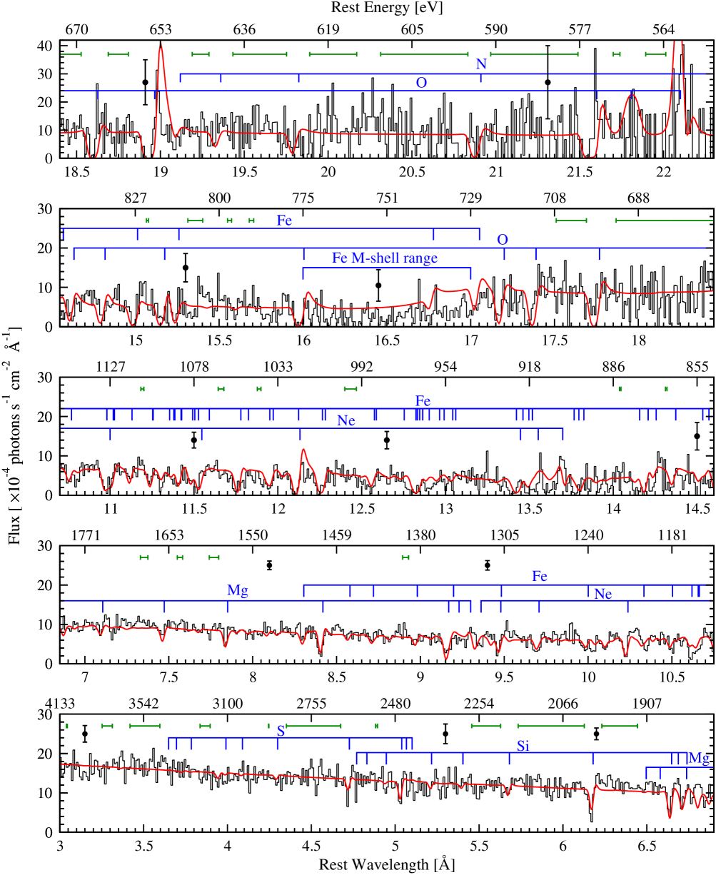
Figure 1: Combined MEG and HEG first-order spectrum of NGC 3783 (black line). Data are binned into 0.01 Å bins and are not smoothed. The spectrum has been corrected for Galactic absorption and the cosmological redshift. Dots with error bars show the typical $\pm 1\sigma$ statistical errors at various wavelengths. The two-component photoionization model discussed in § 5.2.3 is overplotted (red line) to emphasize its good agreement with the data. The H-like and He-like lines of N, O, Ne, Mg, Si, and S, as well as the strongest (EW$>$5 mÅ) Fe lines contributing to the model are marked with blue. The line-free zones are marked as horizontal green ranges.

We note a small ($\approx 20$%) systematic difference in flux between the MEG $+1$st and $-1$st orders around 2.6–2.9 Å where a chip gap is present (at all other chip gaps there is good agreement in flux). However, the effects of the chip-gaps on our combined spectrum are small because of the weighted-mean method we used to derive it: since the numbers of counts in the regions of chip gaps are relatively small (and thus the associated statistical uncertainties are relatively large), these regions receive less weight.

2.2 ASCA

We observed NGC 3783 with ASCA (Tanaka, Inoue, & Holt 1994) in 3 epochs during 2000 January (see Table 1). The multiple observations were designed to provide the time history of the variable ionizing continuum in order to understand better the X-ray emission-line strengths and the state of the object during the Chandra observation. During each ASCA observation the two Solid-state Imaging Spectrometers (known as SIS0 and SIS1; $\approx$ 0.4–10 keV) and the two Gas Imaging Spectrometers (known as GIS2 and GIS3; $\approx$ 0.8–10 keV) were operated. We restrict our analysis of the data from the SIS detectors to that collected in faint mode. The data reduction and screening were performed using ftools (Version 5.0) as described in detail in George et al. (1998a). The total exposure times are listed in Table 1.

During the third observation, which was carried out simultaneously with the Chandra and RXTE observations, there was a severe disruption in the data down-link to a Deep Space Network station (K. Mukai 2000, private communication). About 75% of the data from this observation were lost unrecoverably due to this failure.

2.3 RXTE

An RXTE (Bradt, Rothschild, & Swank 1993) observation was carried out simultaneously with the Chandra observation (see Table 1). Here we present the results from the large-area (0.7 m²) Proportional Counter Array (PCA). The PCA consists of 5 proportional counter units (PCUs) of which only 3 were operational at the time of our observation (units 0, 2, and 3). All PCA count rates in this paper refer to the total counts from these 3 PCUs. We include only data from the upper detection layer as this layer provides the highest S/N for photons in the energy range 2–20 keV.

We reduced the data in the standard way following the RXTE Cook Book. We used standard “good time interval” criteria to select data with the lowest background. We discarded data obtained when the Earth elevation angle was less than 10$\arcdeg$, when the pointing offset from the source was $>0.02\arcdeg$, or when there was significant electron contamination (electron0 $>$ 0.1). We also discarded data obtained during passages through the South Atlantic Anomaly or up to 30 minutes after the peaks of such passages. The PCA is a non-imaging device with a field of view of FWHM $\sim 1\arcdeg$, and the background we subtracted was calculated from a model for a faint source (using the ftools routine pcabackest Version 2.1a).

3 Time Variability

In order to compare the state of the X-ray source in NGC 3783 during the Chandra observation to its state during past years, we use the ASCA observations. For comparison purposes we followed the variability analysis described in George et al. (1998a). We constructed light curves for different energy ranges during each observation. The light curves from SIS0 and  SIS1  and  from  GIS2  and  GIS3  were  added  in  each  case.

Light curves for the three ASCA observations of NGC 3783 carried out in 2000 January. The light curves’ properties were chosen as in George et al. (1998a) to enable comparison to their Figure 1. The adopted bin size is 5760 s which is one ASCA orbit (the good-time interval within one orbit is $\approx 1600$ s). On 2000 January 21 there is a 35 ks gap between the last bin and the preceding one (see § 2.2 for details). Top and middle: Summed light curves obtained for the SIS and GIS detectors. Bottom: Softness ratio (the ratio of the summed count rates observed in the 0.5–2 keV and 2–10 keV bands) for the SIS detectors. Variability is clearly apparent and generally follows the same properties as in George et al. (1998a).

In Figure 3 we present the 0.5–10 keV SIS and 2–10 keV GIS light curves. Variability is apparent both between and within individual observations as was found by George et al. (1998a) for the 1993 and 1996 observations.

During previous ASCA observations the count rates have varied in the ranges of 1.4–3.7 ct s^-1 for the SIS and 1.2–3.0 ct s^-1 for the GIS. The count rate variation ranges of the 2000 observations (2.4–3.7 ct s^-1 for the SIS and 1.3–2.1 ct s^-1 for the GIS) are within the past ranges. Also the softness ratio of the current observation, which varies in the range 0.95–1.25, is consistent with the ranges from the 1993 and 1996 observations (0.8–1.4). The 2000 ASCA observations suggest that the properties of NGC 3783 have remained basically the same, and that during 2000 January (simultaneously with the Chandra observation) NGC 3783 was in a typical, representative X-ray state.

Light curves for the simultaneous observations of 2000 January 20–21 from the three observatories are shown in Figure 3. During the Chandra observation the AGN shows a rise of $\sim$30% in the X-ray flux and then a decrease by about the same amount. The RXTE time variations are consistent with the HEG and MEG variations. The ASCA variations are also consistent with those from the  other two  observatories,  although the live

Light curves from the ASCA SIS (upward pointing triangles; 0.5–10 keV), RXTE PCA (squares; 3–25 keV), Chandra MEG (circles; 0.5–7 keV), and Chandra HEG (stars; 0.5–7 keV). For clarity of presentation the ASCA SIS, RXTE PCA, and Chandra HEG light curves have been divided by factors of 2, 20, and 0.67, respectively. Also shown is the 0.5–7 keV Chandra background light curve (downward pointing triangles) in units of ct s^-1 pixel^-1 which was multiplied by 800000 for clarity.

time of the ASCA observation is very short due to the problem noted in § 2.2. The zeroth-order HETGS image does not contain useful time variation information since it is heavily piled-up, although during the rise in the X-ray flux the pile-up is more severe. For comparison purposes, we also show in Figure 3 a background light curve extracted from a region on the ACIS-S S3 CCD. No significant variations are seen in the background light curve. We have investigated spectral variability during the Chandra observation using hardness-ratio light curves as well as and Kolmogorov-Smirnov tests in wavelength bins with widths comparable to the spectral resolution. We do not find any strong spectral variability that might compromise the spectral analysis below.

4 Modeling the Continuum

4.1 The Chandra Data

The presence of numerous strong absorption lines, emission lines, and absorption edges (see below) complicates the determination of the continuum. To address this issue we introduce the concept of “line-free zones” (LFZs) which are spectral regions free of absorption and emission lines from cosmically abundant elements. The LFZs are crucial for determining the uncertainty on the underlying continuum as a function of wavelength, and hence the uncertainty on the line EWs (§ 5.3).

Figure 2: The solid curves show the 90% confidence contours of the best-fitting parameters associated with the continua as derived using the Chandra LFZs (§4.1) and the 2000 January 21 ASCA and RXTE data (§ 4.2). All three datasets are consistent with a photon index of $\Gamma\approx 1.85$, an ionized column density of $N_{\rm H}\approx 10^{22}\ {\rm cm^{-2}}$, and an ionization parameter of $\log U_{\rm oxygen}\approx{-2}$. The apparent discrepancies in the absolute fluxes of the different missions are discussed in § 4.3. Also shown (dashed) are the contours for the two other ASCA observations made in 2000, and (crosses) the archival ASCA observations from 1996. We stress that the values of $N_{\rm H}$ and $U_{\rm oxygen}$ shown here are only crude parameterizations of the true state of the ionized gas (see § 5.2).

We have determined the LFZs for the MEG and HEG data from the line list used by ion2000 (the 2000 version of ion; see Netzer 1996, and Netzer, Turner, & George 1998). These wavelength ranges (in the rest frame) were then further restricted to allow for intrinsic velocity shifts of $\pm$600 km s^-1 and to account for the resolution of the MEG (i.e., on each side we reduced the LFZs by a distance, in wavelength, of 600 km s^-1 plus 0.023 Å). We also excluded from the LFZs absorption features which are seen in the data but are not included in ion2000 (such as absorption by iron M-shell ions around 16–17 Å; see § 5.3). LFZs at energies above 5 keV were excluded to avoid possible contamination by broad Fe K$\alpha$ emission (§ 7). The LFZs (green horizontal regions in Figure 1) were used on the combined MEG and HEG 1st-order spectrum we derived above in § 2.1. The data within each LFZ were extracted and rebinned such that each new bin contained at least 30 counts. The resulting 315 bins were then fitted using $\chi^{2}$-minimization within the xspec Version 11.0.1 software (Arnaud 1996). It is important to note that the LFZs provide a measure of the observed continuum, which will include spectral curvature resulting from bound-free absorption edges caused by the warm absorber and any “Compton-reflected” continuum at high energies. The spectral model adopted for the LFZs therefore consisted of a power-law continuum (of photon index $\Gamma$), an ionized absorber, and a reflection continuum from neutral material. For simplicity, and to enable easy comparison with the ASCA, RXTE and previous work, in this section we parameterize the ionized absorber using a single-zone model with a column density $N_{\rm H}$ and an ionization parameter $U_{\rm oxygen}$ defined over the 0.538–10 keV band (as described in George et al. 2000). As further discussed in H. Netzer (in preparation) this is a more suitable quantity for parameterizing the state of the ionized gas visible in the Chandra and ASCA bandpasses. We shall discuss this parameterization in the context of our full model in § 5.2. A reflection continuum is required by the RXTE data, but it has a negligible effect on the analysis of the LFZs described here. It is included here for completeness, with its intensity restricted to the range determined from the RXTE data (see §4.2).

We find such a model provides an excellent description of the LFZ data ($\chi^{2}_{\nu}=0.81$ for 310 degrees of freedom; dof). The best-fitting parameters are $\Gamma=1.77^{+0.10}_{-0.11}$, a normalization of $A$(1 keV) $=(1.51^{+0.26}_{-0.22})\times 10^{-2}\ {\rm photon\ cm^{-2}\ s^{-1}\ keV^{-1}}$, $\log N_{\rm H}=21.94^{+0.15}_{-0.20}$ and $\log U_{\rm oxygen}=-2.01^{+0.25}_{-0.28}$. The 90% confidence contours of these parameters are shown in Figure 2, along with those for the other data sets discussed below. We have determined the uncertainty on the observed continuum by fixing each parameter in turn at both its minimum and maximum value consistent with the data at 90% confidence. The spectral analysis was then repeated for each limit on each parameter and the “extreme” spectra determined. These extreme spectra were used to estimate the uncertainties on the line EWs discussed in § 5.3.

4.2 The ASCA and RXTE Data

The ASCA and RXTE observations carried out on 2000 January 21 were largely simultaneous with the Chandra observation (see Table 1 and Figure 3). For ASCA all GIS data below 1 keV were ignored to avoid the uncalibrated degradation of the detectors late in the mission. The SIS data above 0.6 keV were included in the analysis, with their poorly calibrated degradation parameterized using the method outlined in Yaqoob (2000a).

For the analysis presented in this section, the data from both satellites in the 5–7 keV band were again ignored to avoid possible contamination by broad Fe K$\alpha$ emission (see § 7). The spectral model described in § 4.1 (also including Galactic absorption) was applied separately to the ASCA and RXTE data sets. For simplicity, we limit our parameterization of any reflection component to that from neutral material (Magdziarz & Zdziarski 1995) illuminated by an isotropic source above a disk. The intensity of this component is parameterized by the inclination angle, $i$, at which the disk is viewed ($i=0\arcdeg$ for a face-on disk). Acceptable fits for both data sets were obtained.

The bandpass of the RXTE PCA is 3–25 keV, and hence the PCA data are unable to constrain effectively either the ionized absorber or any high-energy cut-off in the underlying continuum. The parameters of the former were therefore fixed to those determined by ASCA (see below), and the cut-off energy was fixed to 200 keV. With these constraints the best-fit model to the PCA has $\chi^{2}_{\nu}=0.93$ (41 dof), $\Gamma=1.86^{+0.03}_{-0.02}$, $A$(1 keV) $=(2.60^{+0.10}_{-0.08})\times 10^{-2}\ {\rm photon\ cm^{-2}\ s^{-1}\ keV^{-1}}$, and $\cos i=0.46^{+0.22}_{-0.14}$. The ASCA data are unable to place a useful constraint on the strength of the reflection component. Thus we restricted the range of $\cos i$ to be that allowed by the PCA data. We obtain $\chi^{2}_{\nu}=1.02$ (483 dof), $\Gamma=1.88^{+0.10}_{-0.12}$, $A$(1 keV) $=(1.99^{+0.32}_{-0.29})\times 10^{-2}\ {\rm photon\ cm^{-2}\ s^{-1}\ keV^{-1}}$ (for SIS0), $\log N_{\rm H}=22.06^{+0.11}_{-0.14}$, and $\log U_{\rm oxygen}=-1.98^{+0.13}_{-0.15}$. These parameters are shown in Figure 2.

Also shown in Figure 2 are the confidence regions obtained by applying the same spectral model to the other two ASCA observations made in 2000 January (dashed curves). Such a model provided acceptable fits to both of the other 2000 data sets ($\chi^{2}_{\nu}$/dof $=$ 1.06/1049 and 1.09/1053 for the January 12 and 16 observations, respectively) with best-fitting spectral shape parameters consistent with those obtained from the January 21 data. The weighted mean values derived from these three ASCA observations are $\Gamma=1.86\pm 0.07$, $\log N_{\rm H}=22.01\pm 0.03$, and $\log U_{\rm oxygen}=-2.07\pm 0.04$.

We have applied the same spectral model to all archival ASCA observations of NGC 3783. This analysis differs from that presented in George et al. (1998b) due to (1) the explicit inclusion of the reflection component, (2) the use of the Yaqoob (2000a) method to account for the degradation of the SIS detectors, (3) the assumption of a single power-law photoionization continuum over the entire 0.1–200 keV band, and (4) the use of $U_{\rm oxygen}$ (0.538–10 keV) rather than $U_{\rm x}$ (0.1–10 keV). Taking into account the turn-up in the spectrum below 0.2 keV assumed by George et al. (1998b), $U_{\rm oxygen}=0.114\,U_{\rm x}$ for $\Gamma=1.77$ (derived from the Chandra spectrum in § 4.1). Our results are generally consistent with those in George et al. (1998b). We find all four 1996 observations to be consistent with $\Gamma=1.85\pm 0.03$, $A$(1 keV) $=(2.21\pm 0.10)\times 10^{-2}\ {\rm photon\ cm^{-2}\ s^{-1}\ keV^{-1}}$, $\log N_{\rm H}=22.15\pm 0.03$, and $\log U_{\rm oxygen}=-1.82\pm 0.01$. These are shown as crosses in Figure 2. The two ASCA observations performed in 1993 have $\Gamma=1.86\pm 0.01$ and $A$(1 keV)$=(1.6$–$1.9)\times 10^{-2}\ {\rm photon\ cm^{-2}\ s^{-1}\ keV^{-1}}$. The O VII and O VIII edges are deeper than those seen at later epochs, and the ionized gas may be parameterized by $\log N_{\rm H}\approx 22.3$ and $-1.9\lesssim\log U_{\rm oxygen}\lesssim-1.8$. However, as found by George et al. (1998b), the spectra at this epoch cannot be adequately modeled by a single-zone ionized absorber.

4.3 Continuum Comparison Between the Satellites

The best-fitting values for $\Gamma$ from the ASCA and RXTE data sets ($\Gamma=1.88^{+0.10}_{-0.12}$ and $\Gamma=1.86^{+0.03}_{-0.02}$, respectively, obtained in § 4.2) are consistent, and they are also consistent with that obtained for the Chandra LFZs in § 4.1 ($\Gamma=1.77^{+0.10}_{-0.11}$). The best-fitting values of $N_{\rm H}$ and $U_{\rm oxygen}$ using the Chandra LFZs and the ASCA data are also consistent (see Figure 2). We find significant differences, however, in the values derived for $A$(1 keV). Presumably these partly result from differences in the absolute flux calibrations of the three missions. Specifically we find the values of $A$(1 keV) derived from the ASCA SIS0, SIS1 and GIS2 detectors to agree within 1%, while that for GIS2 is $\sim 8$% lower. These values are therefore consistent with the quoted uncertainties on the mean absolute flux calibration ($\lesssim 3$%) and internal detector-detector fluctuations ($\lesssim 10$%; Yaqoob 2000b). The value of $A$(1 keV) derived using the RXTE PCA data is $\sim$30% higher than for the SIS0. Such a value is consistent with that expected from the known offset in the absolute calibrations as determined from simultaneous observations of 3C 273; for these the PCA was 30–40% higher than ASCA and BeppoSAX (Yaqoob & Serlemitsos 2000; Yaqoob 2000b).

The value of $A$(1 keV) derived using the LFZs and the Chandra HETGS data is $\approx$25% lower than for the SIS0. To compare better between the Chandra and ASCA data we binned the Chandra spectrum to the ASCA resolution and overplotted it with the ASCA model derived for the 21 January 2000 observation (upper panel in Figure 4.3). The two data sets have good overall agreement in shape, and the systematic shift between them is clearly seen.  The average ratio  between the  Chandra

Upper panel: A comparison of the Chandra spectrum and the ASCA model obtained for the simultaneous observation of 21 January 2000. The Chandra data are binned to the ASCA resolution and are shown as dots with error bars where the horizontal error bar denotes the bin size and the vertical error bar denotes the rms of the data averaged in the bin. Note that the Chandra data are consistent with the presence of ionized edges from O VII and O VIII. Lower panel: The ratio between the Chandra data and the ASCA model presented in the upper panel. The systematic $\approx$ 15% difference is noticeable as well as the 1 keV deficit feature (see § 4.3 for details).

data and the ASCA model is $0.87\pm 0.01$ over the 0.5–7 keV range (lower panel in Figure 4.3; the quoted error is the standard deviation of the mean). The discrepancy is somewhat stronger in the 0.5–2 keV band (ratio of $0.82\pm 0.02$) than in the 2–7 keV band (ratio of $0.90\pm 0.01$). These ratio values are consistent with the Chandra flux calibration uncertainties in the two bands (see § 2.1). However, the shape of the Chandra data to ASCA model ratio along the energy axis suggests this difference between the hard and soft bands might also be a manifestation of the 1 keV deficit feature noted by George et al. (1998a); we further discuss this feature in § 5.3. The average ratio of the Chandra data to ASCA model is smaller than the $A$(1 keV) difference of $\approx$25% stated above. We suggest that the somewhat different values of $N_{\rm H}$, $U_{\rm oxygen}$, and $\Gamma$ between the two data sets contribute to lower the discrepancy seen in $A$(1 keV) by about a factor of 2. This is also seen when comparing the total fluxes measured from the two data sets (after correcting for Galactic absorption). The Chandra observation yields $(2.0\pm 0.2)\times 10^{-11}$ ergs cm^-2 s^-1 in the 0.5–2 keV rest-frame band and $(4.1\pm 0.1)\times 10^{-11}$ ergs cm^-2 s^-1 in the 2–7 keV rest-frame band, while the ASCA observation yields $(2.3\pm 0.2)\times 10^{-11}$ ergs cm^-2 s^-1 and $(4.5^{+0.1}_{-0.2})\times 10^{-11}$ ergs cm^-2 s^-1 in the two bands, respectively (the uncertainties were computed using the extreme spectra described at the end of § 4.1). The differences in the fluxes between the two instruments is $\lesssim 15\%$.

It should be noted that the source exhibits intensity variations during the observations ($\pm 15$%; Figure 3). Since the time-averaged ASCA, Chandra and RXTE spectra sample slightly different times, this may account for at least some of the discrepancies in $A$(1 keV) (e.g., the mean count rate over the whole RXTE observation is $\sim 6$% higher than that during the first two ASCA orbits). We stress that these uncertainties in the flux calibration do not affect the main conclusions of this paper.

The best-fitting continuum models to both the Chandra and ASCA data clearly require O VII and O VIII absorption edges. While these edges, previously found in ASCA data of NGC 3783 and many other AGNs, are not clear on the scale of Figure 1, their influence on the power-law continuum is clearly present in the data, especially in view of the good agreement between the shape of the ASCA model and the Chandra data (see the top panel of Figure 4.3). However, as seen in Figure 1, the high-resolution X-ray spectrum of NGC 3783 has many more features which are blended with these edges.

5 Analysis and Modeling of the Chandra Data

We have modeled the high-resolution Chandra spectra using the basic technique described in Paper I but focusing, this time, on (1) individual spectral features, (2) the line profiles, shifts and EWs, (3) the general physical model, and (4) the spectral energy distribution (SED). The following is a detailed account of the major findings starting with the empirical determination of the absorption-line widths and shifts and ending with global emission and absorption models.

5.1 New Measurements of Absorption Lines

5.1.1 Direct Constraints on the Absorption-Line Widths

There are two ways to obtain the absorption-line widths and their velocity field: (1) direct measurement from the data and (2) a comparison of the observed and modeled EWs (deducing the velocity from the model). Paper I used the second method; this is re-evaluated in § 5.3. Here we demonstrate that the high-resolution spectrum is of high enough quality to resolve some of the absorption lines and obtain direct line-width measurements.

The spectral resolutions of the Chandra gratings are approximately constant with wavelength: 0.023 Å for the MEG and 0.012 Å for the HEG (FWHM of Gaussian profiles). At 15 Å, these correspond to $\approx 460$ km s^-1 for the MEG and $\approx 240$ km s^-1 for the HEG. In Paper I we were not able to constrain directly the velocity dispersion of the absorbing gas because of the poor S/N of individual absorption lines. We have therefore tried a different method of adding several absorption lines from the same element. The advantage is the significant increase in S/N. The disadvantage, the somewhat deteriorated spectral resolution since, for each element, the resolution is then defined by the line with the shortest wavelength.

We created “velocity spectra” by adding, in velocity space, several absorption lines from the same element. The lines were chosen to be the strongest predicted features from a given element and to be free from contamination by adjacent features. The velocity spectra were built up on a photon-by-photon basis (rather than by interpolating spectra already binned in wavelength). The velocity spectra shown in Figure 3 demonstrate the clear detection of absorption lines from oxygen, neon, magnesium and silicon (the ions and lines which are used to create the spectra are listed in the figure). The detection of sulfur absorption is marginal.

We fitted each of the velocity spectra with a Gaussian profile whose centroid and width are free parameters. The resulting centroids and widths ($\sigma$) are listed in Table 2 columns (3) and (4) (the insignificant fit of the sulfur line was omitted from the table). Column (5) of Table 2 lists the expected instrumental $\sigma$ ($\sigma_{\rm instrument}$) for each element computed using the instrumental FWHM resolution (here and elsewhere FWHM=$2.3548\sigma$). The list conservatively refers to the most poorly resolved line, i.e., the one with the shortest wavelength (see Figure 3 for all wavelengths used). For the HEG profiles, $\sigma_{\rm instrument}$ is consistent with $\sigma_{\rm measured}$ for all lines except the neon lines that are apparently resolved. Assuming $\sigma_{\rm true}^{2}=\sigma_{\rm measured}^{2}-\sigma_{\rm instrument}^{2}$, we have proceeded to obtain $\sigma_{\rm true}$, or its upper limit. This is listed in column (6) of Table 2. A few values of $\sigma_{\rm true}$ have upper limits which are lower than the value we find for the neon lines. This may be a result of the conservative instrumental FWHM resolution we used. However, all values of $\sigma_{\rm true}$ are consistent with $\approx 210$ km s^-1 (this value will be used for our model in § 5.2). For the neon lines we find from the HEG $\sigma_{\rm true}=360^{+210}_{-150}$ km s^-1 (i.e., FWHM${}_{\rm true}=840^{+490}_{-360}$ km s^-1). Comparing the $\chi^{2}$ values of our fits to the HEG neon lines we find a $\Delta\chi^{2}$ of 9.3 when allowing the line to be broad (rather than fixing it at the instrumental resolution). According to the $F$-test for 95 dof, this $\Delta\chi^{2}$ corresponds to a highly significant improvement in fit quality at $>99.5$% confidence (see Table C.5 of Bevington & Robinson 1992).

To check for possible problems, we have created two independent velocity spectra for neon from the HEG $+1$st and $-1$st orders. Both are consistent with the presence of line broadening and are consistent with each other. For the HEG $+1$st order, $\sigma_{\rm measured}=374^{+408}_{-193}$ km s^-1 (corresponding to $\sigma_{\rm true}=340^{+427}_{-245}$ km s^-1), and for the HEG $-1$st order, $\sigma_{\rm measured}=390^{+313}_{-186}$ km s^-1 (corresponding to $\sigma_{\rm true}=359^{+327}_{-224}$ km s^-1). As an additional test, we measured the width of the readout trace from the zeroth order image. The PSF of the readout trace (which consists of $\sim 550$ counts) has a FWHM of $2.07\pm 0.20$ pixels. This is broader by 0.5–0.7 pixels than the FWHM of 1.33 pixels reported in the Chandra Proposers’ Observatory Guide or the $1.554\pm 0.013$ pixels derived from a sample of point sources (Sako et al. 2000). We are unable to fully explain the origin of this small discrepancy. It may result from small inaccuracies in the dmregrid software used for the image processing. If this 0.5–0.7 pixel broadening indicates a problem in the aspect reconstruction, it will amount to a velocity broadening of $\sigma$ = 88–123 km s^-1 given the HEG resolution at 9.480 Å (the most poorly resolved neon line we consider). This is small compared with the derived $\sigma$ of neon and does not change the conclusion that the neon lines are resolved. Accounting for such a broadening we obtain FWHM${}_{\rm true}=(792^{+511}_{-402})$–$(817^{+501}_{-378})$ km s^-1.

All line centroids listed in Table 2, column (3), are clearly blueshifted with respect to the systemic velocity. The mean and rms blueshift are $-610\pm 130$ km s^-1. This is consistent with the blueshifts of all the individual features in Table 3 (see below).

Figure 3: (a) MEG and (b) HEG velocity spectra showing co-added lines from oxygen, neon, magnesium, silicon and sulfur. The bin size is 200 km s^-1. The wavelengths of the lines co-added for each element are listed in each panel. Error bars have been computed following Gehrels (1986). Note that absorption is clearly detected from oxygen, neon, magnesium and silicon. There is also a hint of absorption by sulfur, although this is not significant. Note also the P Cygni profile for the oxygen lines. For the HEG we have not shown the co-added velocity spectrum for oxygen, as the photon statistics are poor. Instead, we show a Gaussian absorption line representing the line response function of the HEG at 9.480 Å (the Gaussian FWHM is 364 km s^-1); this is the poorest line response function applicable to the co-added velocity spectrum for neon, shown in the panel immediately below. Note that the neon absorption line appears significantly broader than the line response function. The velocity shifts and dispersions of the UV absorption systems are marked as three horizontal lines in the lower panels.

5.1.2 X-ray P Cygni Profiles

The velocity spectrum of oxygen (the top panel in Figure 3a) also reveals the existence of an emission feature. A half-Gaussian fit to this feature yields a peak at $-100\pm 200$ km s^-1 and a Gaussian $\sigma_{\rm measured}=486^{+237}_{-159}$ km s^-1 (FWHM${}_{\rm true}=1060^{+585}_{-422}$ km s^-1). Thus, we find indications of a P Cygni type profile with an overall width consistent with twice the mean blueshift of the absorption lines. This is the first clear detection of an X-ray P Cygni profile from an extragalactic source and one of the first P Cygni profiles in X-ray astronomy (see Brandt & Schulz 2000). This profile will be used as input to our global emission and absorption model.

Table 2: Fitting of Added Absorption-Line Profiles

		Line centroid	$\sigma_{\rm measured}$	$\sigma_{\rm instrument}$	$\sigma_{\rm true}$
Element	Spectrum	(km s-1)	(km s-1)	(km s-1)	(km s-1)
(1)	(2)	(3)	(4)	(5)	(6)
O	MEG	$-715^{+132}_{-151}$	$282^{+131}_{-105}$	183	$<370$
Ne	HEG	$-685^{+178}_{-181}$	$390^{+197}_{-132}$	155	$358^{+209}_{-152}$
Ne	MEG	$-668^{+68\phantom{0}}_{-69\phantom{0}}$	$292^{+91\phantom{0}}_{-77\phantom{0}}$	309	$<226$
Mg	HEG	$-502^{+64\phantom{0}}_{-63\phantom{0}}$	$217^{+81\phantom{0}}_{-56\phantom{0}}$	206	$<215$
Mg	MEG	$-493^{+89\phantom{0}}_{-91\phantom{0}}$	$420^{+99\phantom{0}}_{-81\phantom{0}}$	412	$<315$
Si	HEG	$-461^{+103}_{-121}$	$376^{+163}_{-113}$	281	$<459$
Si	MEG	$-777^{+116}_{-123}$	$562^{+182}_{-145}$	562	$<488$

^aCorresponds to Figure 3.
Note. — Uncertainties are 90% confidence for one parameter of interest ($\Delta\chi^{2}~{}=~{}2.71$).

We note that the averaging procedure above, consisting of several lines from each series, tends to reduce the contrast between the emission and absorption features for all lines with large optical depths; the absorption EW is roughly constant for all such lines while the emission EW is always the largest for the first line in the series (e.g., the Ly$\alpha$ line in the H-like ions). This is the reason why only the strongest emission lines, those due to oxygen, are seen in the velocity spectra. However, we detect individual P Cygni line profiles in other elements [e.g., Ne X (12.132 Å), Si XIII (6.648 Å); see Figure 1].

The broken power-law continuum used in the modeling described in § 5.2 and detailed in Table 4. The Chandra and HST STIS observable ranges are marked with double-headed arrows. The unobservable part of the continuum due to the Galactic column density is between the two vertical dashed lines; see § 6.1.

5.2 Photoionization Models

5.2.1 Model Parameters and Line Widths

We proceed by calculating a number of photoionization models that are compared, in turn, to the observed spectrum. The basic assumptions are outlined in Paper I, but we list them here for completeness.

All models consider one or more outflowing shells of constant density, solar metallicity, highly ionized gas (HIG). We assume this gas is in photoionization and thermal equilibrium. The HIG is illuminated by a central broken power-law continuum of photon index $\Gamma$ as defined in Table 4 and illustrated in Figure 5.1.2. The choice of the 0.1–50 keV slope of $\Gamma=1.77$ is the result of experimenting with a range of models, as explained in § 4.1 and later in this section. The very sharp decline over the 40–100 eV range is consistent with the expected $\sim 10^{5}$ K accretion disk temperature. The other parameters of the model are the column density, covering fraction and ionization parameter for each shell.

In Paper I we used the 0.1–10 keV ionization parameter $U_{\rm x}$. For a simple power-law spectrum with $\Gamma=1.77$, $U_{\rm oxygen}=0.252\,U_{\rm x}$. We also define the internal microturbulence velocity which is added, in quadrature, to the locally computed thermal velocity of the ions, $V^{2}=V^{2}_{\rm thermal}+V^{2}_{\rm turbulence}$ (these are Doppler profiles; i.e., the velocity $V$ is given by $V=\sqrt{2}\sigma$). This defines the line widths and is an important factor which determines the line EWs. We note that $V_{\rm thermal}\ll V_{\rm turbulence}$ in our model as the temperature of the gas is $\approx 10^{5}$ K.

The model of Paper I included a single-component HIG with a large covering fraction, a column density of $\log N_{\rm H}=22.1$, solar metallicity, and an ionization parameter of $U_{\rm x}=0.13$ ($U_{\rm oxygen}=0.01$). A closer examination of this model shows that, while the fit to the continuum level and the O VII and O VIII bound-free absorption features is satisfactory, there are three fundamental problems: (1) the assumed microturbulence velocity of 150 km s^-1 underpredicts the EWs of several neon and magnesium absorption lines, (2) the EWs of several high-energy absorption lines [e.g., Si XIV (6.180 Å)] are underpredicted by factors of at least 3, and (3) the model made no attempt to explain the rich spectrum of iron L-shell lines.

Regarding point (1), we note that the calculations presented in Paper I contained a factor of 1.7 error in the model EW calculations. Thus, the EWs quoted there as corresponding to a microturbulence velocity of 150 km s^-1 correspond, in fact, to a microturbulence velocity of about 250 km s^-1. The more detailed fitting in § 5.1.1 indicates that even a somewhat larger velocity is likely. In the following we adopt as our standard $V_{\rm turbulence}=300~{}{\rm km\,s}^{-1}$ ($\sigma\approx 210~{}{\rm km\,s}^{-1}$). Regarding point (2), several attempts to change the microturbulence velocity, the column density, and the ionization parameter show that no model can explain the EWs of the high-ionization species and, at the same time, keep the good fit of the EWs of many lower ionization lines. We are driven to the conclusion that modeling the observed spectrum requires more than one absorbing component. In § 5.2.3 we describe our attempts to fit a multi-component model to the spectrum of NGC 3783. As for point (3), we have considerably modified ion (into ion2000) to include hundreds of new iron lines, as explained in § 5.2.2.

5.2.2 The Iron L-Shell Lines

ion2000 includes substantial improvements to its atomic data base designed to model the numerous iron L-shell absorption features apparent in the spectrum. Atomic calculations have been performed using the multi-configuration, relativistic Hebrew University Lawrence Livermore Atomic Code (hullac) developed by Bar-Shalom, Klapisch, & Oreg (2001). In this code, the energy levels are calculated with the relativistic version of the parametric potential method (Klapisch et al. 1977), including configuration mixing. Subsequently, the oscillator strengths for the radiative transitions are computed using first-order perturbation theory.

Photon impact processes involving L-shell (i.e., the $n=2$ electronic shell, where $n$ is the principal quantum number of the electrons in the outermost occupied orbital of the ion in its ground state) excitations are computed for Fe XVII through Fe XXIV. All of the important transitions from $n$ to $n^{\prime}$ ($n^{\prime}$ $\geq$ 3) are taken into account, of which the 2p–3d excitations are the strongest and, therefore, those clearly observed in the spectrum. Only excitations from the ground level of each shell are included, except for Fe XIX, in which the first excited level can be significantly populated even at relatively low densities. Consequently, absorption processes from that excited level of Fe XIX are also calculated. This feature of Fe XIX can potentially provide a density diagnostic at densities of order $10^{9}$ cm^-3 (the precise density is somewhat uncertain due to uncertain atomic data), since the EWs for absorption lines from this excited level depend strongly on the density of the absorbing medium (see § 5.3).

The new set of oscillator strengths obtained in this way are used to compute the optical depths of several hundred iron L-shell lines contained in ion2000. In two recent works, similar atomic data for the Fe L-shell transitions were used for line-by-line analysis of high-resolution spectra of emission (Behar, Cottam, & Kahn 2001) and absorption (Sako et al. 2001) lines. In those studies good agreement was found between the calculations and the observations.

5.2.3 Two-Component Models

We have experimented with several two-component models. These include two distinct shells situated at different radial locations that are characterized by different column densities and ionization parameters. Guided by the good continuum fit (§ 4.1), we have explored the following range of parameters (which is not necessarily unique): $\Gamma=1.77\pm 0.1$, $\log N_{\rm H}={22.1\pm 0.2}$, and $\log U_{\rm oxygen}$ from $-1.824$ to $-0.700$. A possible combination that gives good agreement with the observations (see § 5.3) is made of the following components:

The low-ionization component

with $\log U_{\rm oxygen}=-1.745$, a hydrogen column density of $\log N_{\rm H}=22.2$, a global covering factor of 0.5 and a line-of-sight covering factor of unity.

The high-ionization component

with $\log U_{\rm oxygen}=-0.745$, a hydrogen column density of $\log N_{\rm H}=22.2$, a global covering factor of 0.3, and a line-of-sight covering factor of unity.

The gas density in both components is assumed to be $10^{8}$ cm^-3. This density is high enough so that $\Delta R\ll R$, where $R$ is the distance to the continuum source and $\Delta R$ is the shell thickness. We have no real constraints on the density (except that it must exceed about $10^{4}$ cm^-3 to justify the thin shell approximation) and hence no way to calculate the masses of these components. Under our assumptions the low-ionization component is further away from the source and is thus illuminated by the radiation passing through the high-ionization shell. However, the high-ionization component is almost transparent to continuum radiation from the source, and due to the spectrally distinct line features of the two components, we can neglect the changes in the illuminating spectrum for the (outer) low-ionization shell. The two components are assumed to have the same outflow and microturbulence velocities which is consistent with the observations. The EW calculations listed in § 5.3 are made under the assumption of no velocity shift between the two components.

5.2.4 Continuous Flow Models

We have also tested continuous models made out of a single outflowing component of HIG. In this case, geometrical dilution is important, and different radial locations are characterized by different ionization parameters. We assumed a density law of the form $N(R)\propto R^{-\alpha}$ with $\alpha<2$. Thus the ionization level decreases outward, and the global properties resemble the two distinct component model. The requirement of achieving a factor $\gtrsim 10$ reduction in $U_{\rm oxygen}$, due to geometrical dilution, with a restricted range in column density, introduces a constraint on the value of $N_{0}R_{0}$ where the subscript zero refers to conditions at the base of the flow. This results in a low density gas whose total mass exceeds, by several orders of magnitude, the masses of the two distinct high density shells in § 5.2.3 (the mass is roughly proportional to $1/N$).

While there are several combinations of $\alpha$ and minimum distance that satisfy these conditions and give the required range of ionizations, the overall fit to the data for the combinations we have tried is inferior to the fit of the two-component model. We have therefore decided not to present these fits in detail. We emphasize that models of this kind need further investigation, but this is beyond the scope of this paper.

Table 3: Absorption and Emission Lines from NGC 3783

Measured $\lambda$	Model $\lambda$	Measured EW	Model EW	Ion name and
(Å)	(Å)	(mÅ)	(mÅ)	transition rest-frame wavelength (Å)
(1)	(2)	(3)	(4)	(5)
04.717	04.718	$7.8\pm 9.3$	$4.5$	S XVI (4.727)
05.029	05.028	$\phantom{0}8.2\pm 11.3$	$8.2$	S XV (5.039)
06.171	06.170	$17.9\pm 5.1\phantom{0}$	$11.2$	Si XIV (6.180)
06.636	06.637	$11.1\pm 4.5\phantom{0}$	$16.5$	Si XIII (6.648)
06.681	06.668	$-10.6\pm 9.1\phantom{string}$	$-1.5$	Si XIII (6.648)
06.707	06.711	$5.9\pm 5.0$	$11.4$	Si XII (6.720)
07.094	07.094	$2.9\pm 5.7$	$6.0$	Mg XII (7.106)
07.163	$\cdots$	$6.5\pm 2.6$	$\cdots$	Al XIII (7.18)
07.462	07.461	$\phantom{0}4.5\pm 10.1$	$9.8$	Mg XI (7.473)
07.744	$\cdots$	$3.8\pm 4.3$	$\cdots$	Al XII (7.76)
07.838	07.837	$7.5\pm 4.7$	$15.2$	Mg XI (7.851)
08.403	08.404	$24.3\pm 5.6\phantom{0}$	$15.6$	Mg XII (8.419)
09.156	09.153	$26.5\pm 9.2\phantom{0}$	$26.4$	Mg XI (9.169)
09.305	09.293	$-9.1\pm 14.3$	$-6.9$	Mg XI (9.300)
09.356	09.327	$9.5\pm 9.0$	$10.8$	Ne X (9.362), Mg X (9.336)
09.460	09.466	$12.0\pm 6.1\phantom{0}$	$14.0$	Ne X (9.480), Fe XXI (9.483)
09.517	09.500	$-18.6\pm 17.0\phantom{string}$	$-2.3$	Ne X (9.480), Fe XXI (9.483)
09.692	09.692	$22.2\pm 8.0\phantom{0}$	$12.4$	Ne X (9.708)
09.734	09.740	$-6.4\pm 12.1$	$-3.5$	Ne X (9.708)
09.984	09.985	$14.9\pm 16.2$	$9.8$	Fe XX (9.999, 10.001, 10.006)
10.032	10.042	$17.3\pm 13.7$	$6.0$	Fe XX (10.040, 10.042, 10.054, 10.060)
10.100	10.100	$14.7\pm 12.0$	$10.8$	Fe XVII (10.112)
10.223	10.223	$18.2\pm 8.5\phantom{0}$	$19.6$	Ne X (10.238)
10.275	10.264	$-23.7\pm 22.1\phantom{0}$	$-2.4$	Ne X (10.238)
10.345	10.317	$12.8\pm 13.0$	$9.7$	Fe XVIII (10.361, 10.363, 10.365)
10.500	10.488	$13.1\pm 12.5$	$10.4$	Fe XVII (10.504)
10.624	10.629	$46.6\pm 10.9$	$20.3$	Fe XVII (10.657), Fe XIX (10.650, 10.642, 10.630, 10.631, 10.641)
10.754	10.753	$15.9\pm 23.5$	$13.7$	Fe XVII (10.770)
10.798	10.809	$15.5\pm 8.2\phantom{0}$	$4.1$	Fe XIX (10.828)
10.978	10.981	$43.7\pm 11.7$	$53.5$	Ne IX (11.000), Fe XXIII (10.981, 11.019), Fe XVII (11.026)
11.119	11.116	$11.2\pm 20.2$	$15.7$	Fe XVII (1113.9)
11.236	11.237	$15.7\pm 13.3$	$22.0$	Fe XVII (11.254)
11.302	11.302	$24.8\pm 10.8$	$13.0$	Fe XVIII (11.326, 11.319, 11.315)
11.404	11.406	$17.7\pm 21.0$	$18.7$	Fe XXII (11.427), Fe XVIII (11.423)
11.476	11.482	$18.3\pm 18.2$	$16.7$	Fe XXII (11.492, 11.505)
11.517	11.527	$25.7\pm 10.7$	$31.9$	Ne IX (11.547)
11.750	11.758	$41.0\pm 10.0$	$33.3$	Fe XXII (11.780)
11.948	11.947	$31.8\pm 11.7$	$27.6$	Fe XXI (11.952, 11.973)
12.101	12.106	$44.8\pm 8.1\phantom{0}$	$39.2$	Ne X (12.132), Fe XVII (12.124)
12.147	12.153	$-7.8\pm 15.1$	$-46.1$	Ne X (12.132)
12.251	12.255	$49.4\pm 9.9\phantom{0}$	$42.0$	Fe XVII (12.266), Fe XXI (12.284)
12.556	12.556	$37.8\pm 12.6$	$16.9$	Fe XX (12.576, 12.588)
12.809	12.823	$60.3\pm 14.0$	$49.5$	Fe XX (12.846, 12.864, 12.903)
13.399	13.422	$57.4\pm 21.8$	$49.1$	Ne IX (13.447)
13.495	13.491	$52.3\pm 17.1$	$18.2$	Fe XIX (13.518, 13.497)
13.567	13.564	$-18.9\pm 26.3\phantom{0}$	$-23.4$	Ne IX (13.553)
13.694	13.680	$-44.3\pm 39.8\phantom{0}$	$-22.5$	Ne IX (13.699)
13.777	13.798	$33.5\pm 17.1$	$32.6$	Fe XVII (13.825)
14.181	14.183	$33.5\pm 18.9$	$26.5$	Fe XVIII (14.208)
14.342	14.348	$28.5\pm 39.8$	$21.9$	Fe XVIII (14.373)
14.505	14.508	$37.2\pm 13.6$	$22.7$	Fe XVIII (14.534)
14.622	14.605	$21.6\pm 23.4$	$27.1$	O VIII (14.635)
14.807	14.792	$18.7\pm 20.3$	$37.1$	O VIII (14.820)
14.988	14.987	$30.7\pm 24.8$	$53.2$	Fe XVII (15.014)
15.157	15.153	$22.9\pm 30.9$	$46.2$	O VIII (15.176)
15.233	15.236	$19.7\pm 18.9$	$33.0$	Fe XVII (15.261)
15.977	15.975	$47.2\pm 16.0$	$54.1$	O VIII (16.006)
17.163	17.168	$28.9\pm 15.5$	$39.2$	O VII (17.20)
17.340	17.367	$46.8\pm 19.5$	$39.8$	O VII (17.39)
17.730	17.733	$24.2\pm 32.1$	$56.3$	O VII (17.768)
17.789	17.794	$-9.9\pm 25.5$	$-17.0$	O VII (17.768)
18.597	18.593	$29.6\pm 13.0$	$65.8$	O VII (18.628)
18.659	18.662	$-30.4\pm 58.6\phantom{0}$	$-10.7$	O VII (18.628)
18.926	18.927	$60.2\pm 20.6$	$73.3$	O VIII (18.967)
18.981	19.001	$-51.1\pm 57.8\phantom{0}$	$-244.4$	O VIII (18.967)
21.538	21.557	$56.1\pm 47.9$	$87.0$	O VII (21.602)
21.594	21.635	$-68.4\pm 83.4\phantom{0}$	$-63.5$	O VII (21.602)
21.808	21.814	$-38.1\pm 373.7$	$-183.1$	O VII (21.807)
22.113	22.087	$-161.8\pm 180.7\phantom{0}$	$-393.8$	O VII (22.101)

^aA negative sign before an EW indicates an emission line.
^bUncertainties are $\pm 0.01$ Å.
^cLine not included in our model.

5.3 Comparison with the Observations

The success of the two-component model of § 5.2.3 has been evaluated in two ways. First, we compare the observed and calculated EWs of as many lines as we can reliably measure. Here the number of lines is about 62 compared with the 28 lines used in Paper I. Most of the difference is due to the iron L-shell lines now having been computed with more reliable oscillator strengths. Second, we inspect individual, small wavelength bands by overlaying the computed model on the observed spectrum. This is particularly important in those regions containing a large number of emission and absorption lines; some of these are so crowded that there is no direct way to separate the different contributions to the various blends (see, for example, the line complex over the 9–17 Å range in Figure 1 with dozens of Fe XVII to Fe XXIV absorption lines). Direct visual inspection is the best way to assess the validity of the model in this case.

The visual evaluation method is illustrated in the various panels of Figure 1 where we overlay the computed spectrum (red curve) on the observed one (black curve). This is done after a three-stage convolution process to produce the computed line profiles. First, each line is convolved with the microturbulence velocity representing the local line broadening. Next, we convolve the emission lines with a boxcar profile of 1220 km s^-1 width, centered on the systemic velocity and representing the 610 km s^-1 outflow assumed for both absorption components. We also take into account the absorption of the emission-line photons by the line-of-sight outflowing gas which gives the correct P Cygni type profile. Finally, we convolve the entire theoretical spectrum with a constant-wavelength width Gaussian (0.023 Å), to account for the MEG resolution used for the visual comparison method.

The result of the comparison is quite satisfactory. The theoretical model fits the observed spectrum over most bands and most absorption lines. In particular, we are able to adequately fit $\sim 50$ absorption lines, including some 30 iron L-shell lines, taking into account line blends. Most, but not all, emission lines also show a reasonable fit. Unfortunately, most emission lines are so weak that the quality of the fit is not, by itself, a very conclusive result.

There are several notable discrepancies deserving comment:

1. Three emission lines clearly show small EWs compared with the model predictions. These are O VII (21.807, 22.101 Å) and O VIII (18.967 Å). The discrepancy might result from low S/N and the poor flux calibration at those wavelengths (see § 2.1). In fact, for two of the three lines, the predicted EWs are within the uncertainty of the observed lines.

2. There is a noticeable broad absorption feature at around 16–17 Å that looks like a blend of many absorption lines. Sako et al. (2001) have recently observed a similar, but much stronger, absorption feature in the X-ray spectrum of the quasar IRAS 13349+2438 and have identified it as an unresolved transition array of 2p-3d inner-shell absorption lines by iron M-shell ions (Fe IX–Fe XIV) in a relatively low-ionization medium. Those authors have tentatively associated this absorption with the ionized skin of a dusty torus surrounding the AGN. Such absorption is not included in ion2000. We have verified that the abundances of these ions in the low-ionization component are, indeed, large enough to produce the needed extra absorption. We will make additional checks when better S/N data become available.

3. There is a notable discrepancy between the model and the observations at the Si XI (6.813 Å) line. While the model predicts absorption, the observations show an emission line at the same energy. Both the energy and the oscillator strength of this line are uncertain, and this might be the source of the discrepancy.

We have measured the absorption and emission features in the observed spectrum using the underlying continuum from the fitted model (§ 4.1). Line EW measurements, together with the model EWs, are presented in Table 3. In columns (1) and (2) we list the observed wavelengths and the wavelengths measured from the model, respectively. The observed EWs and the derived uncertainties are listed in column (3). A negative sign before an EW indicates an emission line. The EW uncertainties take into account the uncertainty in the continuum placement (§ 4.1) combined in quadrature with uncertainties due to the number of counts in the line. These uncertainties can be used to assess the realities of the various lines. In column (4) we give the EW as measured from our model, and in column (5) we identify the main ions contributing to the line or blend, based on the model and the measured energy. The model wavelengths (column 2) and EWs (column 4) were measured directly from the modeled spectrum (red line in Fig 1) since any attempt to calculate them is hindered by the blending of the many components, as explained above. The model does not include the Al XIII (7.18 Å) and Al XII (7.76 Å) lines which are tentatively identified in the data.

Comparing the observed and the modeled wavelengths, we find good agreement. The mean and rms velocity shift between the two is $-1\pm 267$ km s^-1 for the 67 lines ($-22\pm 245$ km s^-1 for the 53 absorption lines and $75\pm 338$ km s^-1 for the 14 emission lines). The $\chi^{2}$ between the observed wavelengths and the modeled ones is 88.7 for the 67 lines. As there is only one free parameter (the 610 km s^-1 outflow velocity), we have 66 dof and the reduced $\chi^{2}$ is 1.32. This confirms that the adopted velocity shifts for the absorption and emission features are in good agreement with the observation. We checked the velocity shifts of lines which primarily originate from the low-ionization component of our model versus lines which primarily originate from the high-ionization component. The two ionization components are not dynamically distinguishable within the uncertainties of our data.

Figure 5.3 compares the observed EWs with those derived from the model (columns 3 and 4 of Table 3) except for three low-energy emission lines (see above). The agreement between the two is very good, both for the emission and absorption lines, as shown by the spread along a line with slope unity. In particular, all strong lines predicted by the model are observed. The $\chi^{2}$ between the observed EWs and the modeled ones is 69.7 for the 67 lines shown. The number of free parameters in our model is 6 (density, column density, ionization parameter, microturbulence velocity, and global covering factors for the two components), so the reduced $\chi^{2}$ is 1.14.

Our estimate for the global covering factor is based on the emission-line intensities which, as explained earlier, are highly uncertain (see Table 3). A reasonable range for the covering factor, which is consistent with all measured EWs, is 0.2–0.7. We have also verified visually that covering factors of 0.5 and 0.3 (for the low-ionization and high-ionization components, respectively) give the best fit to the emission lines at shorter wavelengths ($\lambda<16$Å), where the S/N is better.

The 1 keV deficit feature which was noted by George et al. (1998a) and seems also to exist in our comparison between the Chandra data and ASCA model (bottom panel of Figure 4.3) can be explained by many iron L-shell absorption lines around 1 keV.  These lines were not present in the modeling of George et al. (1998a), and they probably cause in part the 1 keV deficit feature. George et al. (1998a) suggested there might be two

Measured EWs versus model EWs. The positive EWs are for the absorption lines, and the negative EWs are for the emission lines. All identified lines from Table 3 except for 3 emission lines are plotted here (see § 5.3 for details). A line with a slope of unity is drawn to guide the eye.

TABLE 4
Model SED $E_{1}$ $E_{2}$ $\Gamma$ 0.2 eV 02 eVstring 2.00 string2 eV 40 eVstring 1.50 string40 eV 0.1 keV 5.77 00.1 keV string50 keV 1.77 string50 keV 001 MeV 4.00

or more zones of photoionized material, which are changing in time, to explain this deficit. This is also reinforced by the good fit of our two component model. We showed that two absorption components are needed to explain the observed richness of the absorption lines.

As mentioned in § 5.2.2, some Fe XIX lines can provide important density diagnostics, since they arise from an excited fine-structure level with a critical density of order $10^{9}$ cm^-3. We have constructed several high-density models and searched for the strongest fine-structure lines in our data (at 13.46 and 13.96 Å). We found that either the lines are blended with other L-shell lines or else the S/N is not adequate to conduct the test. Much better S/N observations, and sole use of the HEG to keep the highest possible resolution, are required. The current observations are inadequate.

6 UV Absorption Toward NGC 3783

6.1 The Associated UV Absorber

Many Seyfert 1 galaxies containing ionized X-ray absorbers also show strong, narrow, UV absorption lines (e.g., Crenshaw et al. 1999 and references therein). These features seem to vary in EW and velocity shift on time scales of weeks to months. The suggestion that the lines originate from the same component producing the strong X-ray absorption (Mathur et al. 1994) has been tested in many papers (e.g., Mathur, Elvis, & Wilkes 1995; Shields & Hamann 1997) without conclusive results. The main unknowns were the SED at far-UV energies (see Figure 5.1.2), responsible for the ionization of the observed UV species, and the poor X-ray spectral resolution.

In Paper I we compared the high-resolution Chandra spectrum of NGC 3783 with a UV spectrum taken $\approx 5$ yr earlier. We found that the shifts and velocity dispersions of the X-ray absorption lines were consistent with those observed for the UV lines. However, the calculated warm absorber model of Paper I resulted in column densities for C IV and N V that were 37 and 5 times too small, respectively, when compared with the values deduced from UV observations. We also commented on the fact that the expected column densities for C IV and N V are very sensitive to the unknown Lyman continuum SED.

We have looked again at this issue trying to resolve it in light of newly available UV observations and the improved X-ray models. First, we compare our Chandra spectrum with HST STIS spectra obtained 37 days later (Crenshaw et al. 2000). The new UV observation shows 3 absorption-line systems blueshifted with respect to the systemic velocity by $\approx$ $-$560, $-$800, and $-$1400 km s^-1. These systems have velocity dispersions of 160, 220, and 210 km s^-1, respectively. Thus, the 2000 UV observation is consistent with the Chandra line shifts, but the UV line widths seem to be narrower than at least the resolved neon X-ray lines. We also note that, in the 2000 UV observation, the $\approx-1400$ km s^-1 component became much stronger and is present also in Si IV, indicating a lower ionization state compared to the other components. It is very unlikely that such a system will also show strong X-ray lines. Looking at Figure 3, we see no highly significant evidence for such absorption system in the X-ray spectrum.

We have looked at the UV lines predicted from our lower-ionization shell. For this component we now find EW(C IV)= 0.6 Å and EW(N V)=3.1 Å, entirely consistent with the UV observations of Crenshaw et al. (1999) and superficially confirming the idea that the UV and X-ray lines originate from the same component. However, as explained briefly in Paper I, this result is extremely sensitive to the ratio of the far-UV to 0.1–10 keV flux. The SED assumed in Paper I contained a much larger far-UV flux compared to the one assumed here. As a result, the C IV and N V absorption lines were much weaker than for the current SED.

To verify the above conclusion, we have renormalized the UV-to-X-ray continua in several different ways by changing the parameters of the assumed SED from 40–200 eV (see Table 4 and Figure 5.1.2). Moving only one point, at 0.1 keV, to 0.2 keV (while keeping the X-ray slope unchanged at $\Gamma=1.77$) leads to a reduction by a factor of 3 in EW(C IV) and a factor of 2.3 in EW(N V). A further move of the point at 40 eV to 60 eV, keeping the UV slope unchanged ($\Gamma=1.5$; see Table 4) results in further reductions by factors of 4 and 1.4 in EW(C IV) and EW(N V), respectively. Both changes do not influence the chosen value of $U_{\rm oxygen}$ and have no effect on the calculated X-ray line EWs. Thus the EWs of the UV absorption lines are extremely sensitive to the exact cut-off frequency of the unobserved UV continuum. They are also sensitive, by a lesser amount, to the relative UV-to-X-ray normalization. The conclusion is that there is little one can infer from the comparison of the available UV and X-ray observations regarding the relationship between the UV and X-ray absorbers. Part of the solution is to obtain real simultaneous observations. These will give the simultaneous EWs for the X-ray and UV lines and some handle on the relative UV and X-ray continuum fluxes.

6.2 The High-Velocity Cloud Toward NGC 3783

Toward the direction of NGC 3783 there is a high-velocity cloud (HVC) denoted HVC 287.5+22.5+240 (Lu et al. 1998 and references therein). HVCs are H I clouds moving at velocities inconsistent with simple models of Galactic rotation and are generally defined as having velocities exceeding 90 km s^-1. The HVC toward NGC 3783 has a velocity of 240 km s^-1 with respect to the local standard of rest and is at a distance of 10–50 kpc. In addition to H I absorption it was found to have absorption by S II and Fe II. We find it unlikely that the absorption we report on in this paper has anything to do with this HVC for several reasons: (1) the velocity of this HVC is an order of magnitude less than the redshift velocity of NGC 3783, corresponding to $\approx 4$ resolution elements of the MEG at 10 Å, (2) the column densities derived for this HVC [$N$(H I) = $(8\pm 1)\times 10^{19}$ cm^-2, $N$(Fe II) = $(8.5\pm 1.0)\times 10^{13}$ cm^-2, and $N$(S II) = $(3.7\pm 1.0)\times 10^{14}$ cm^-2] are about two orders of magnitude smaller than the column densities indicated from the NGC 3783 spectrum, and (3) in the HVC there is no source of radiation to cause the high degree of ionization needed to produce the ions detected in the NGC 3783 spectrum.

7 The Iron K$\alpha$ Line

At least some of the Fe K$\alpha$ fluorescent line emission seen from Seyfert 1 galaxies is often very broad and is generally interpreted as originating from an accretion disk orbiting around a central black hole (e.g., Fabian et al. 2000 and references therein). The profile of the line is assumed to reflect gravitational and Doppler effects within a few tens of gravitational radii of the black hole. As narrow Fe K$\alpha$ line emission is also expected from matter beyond the accretion disk, it is important to separate the narrow emission from the broad emission. The spectral resolution of pre-Chandra X-ray missions was not high enough to resolve the narrow component from the broad one (e.g., the $\sim$ 160 eV FWHM of ASCA is too poor for that task), and currently only the Chandra HETGS is capable of such separation (with a factor of $\sim 4$ better spectral resolution at Fe K$\alpha$ than ASCA).

Figure 4: The observed ratios of the data to the underlying continua near the Fe K$\alpha$ line, along with model predictions (bold line; convolved with the appropriate instrumental response) discussed in the text. For ASCA, the mean ratio is shown for the SIS detectors for all observations at each epoch, rebinned for clarity. Fe K$\beta$ is included at 7.06 keV with a flux that is 11% that of Fe K$\alpha$. a) The model prediction for a narrow Gaussian Fe K$\alpha$ line at 6.4 keV and a flux of $6.6\times 10^{-5}$ photons cm^-2 s^-1 as described in § 7.1. Such a model provides an adequate description of the Chandra and 2000 ASCA data sets. However, the 1996 ASCA data show an excess in the red wing of the line. b) The model prediction for a narrow Gaussian plus a 6.4 keV Schwarzschild “diskline” where the disk is inclined at an angle $i=30\arcdeg$ and the line emissivity $\propto r^{-3}$ between 6 and $10^{3}$ $r_{\rm g}$ (see § 7.2). In the upper two panels the narrow component has a flux of $6.6\times 10^{-5}$ photons cm^-2 s^-1 and the broad component $5.0\times 10^{-5}$ photons cm^-2 s^-1 (the maximum intensity consistent with the data). In the lower panel, the narrow and broad components have fluxes $4.2$ and $12\times 10^{-5}$ photons cm^-2 s^-1, respectively (see § 7.2).

7.1 The Narrow Component

The narrow Fe K$\alpha$ line from NGC 3783 is very prominent in the Chandra HETGS spectrum (Figure 4a). The line peak is at $6393\pm 15$ eV, consistent with Fe i–xii. Modeling the line in the combined spectrum as a single Gaussian, we find a FWHM of $26\pm 10$ mÅ which is consistent with the line not being resolved at the resolution of the MEG. The line flux is $(6.6\pm 2.1)\times 10^{-5}$ photons cm^-2 s^-1 $=$ $(6.8\pm 2.2)\times 10^{-13}$ ergs cm^-2 s^-1, corresponding to an EW of 35$\pm$11 mÅ ($115\pm 36$ eV) as measured against the underlying continuum. Investigating the HEG spectrum alone, the FWHM of the line is $15\pm 6$ mÅ. This FWHM is consistent with the HEG resolution of 12 mÅ  and thus the line has a FWHM of less than 3250 km s^-1. This velocity is comparable to, or lower than, the velocity of the BLR of this object which is $\sim$ 4000 km s^-1 (Reichert et al. 1994; Wandel, Peterson, & Malkan 1999; FWHM${}_{\rm H\beta}=4100\pm 1160$ km s^-1). Given this upper limit on the narrow Fe K$\alpha$ width, and assuming a simple correlation of line width with radial location in a Keplerian system, we conclude that the origin of this feature is anywhere from just outside the BLR to as far as the NLR. In particular, the observed energy and large EW suggest that the line may arise in the putative torus.

Ghisellini, Haardt, & Matt (1994) and Krolik, Madau, & Zycki (1994) have calculated the X-ray line emission expected from putative obscuring tori in AGNs. Both studies predict the Fe K$\alpha$ line to have a characteristic EW of $\sim 100$ eV for a torus which has an opening angle of $\sim 35\arcdeg$, an inclination angle to the line of sight of $\lesssim 35\arcdeg$, and a column density $N_{\rm H}\gtrsim 10^{24}$ cm^-2. Later, Matt, Brandt, & Fabian (1996) considered changes in the line EW for various metalicities. All predicted EWs are in agreement with the one measured here and suggest that the narrow Fe K$\alpha$ line from NGC 3783 could arise from the torus.

In a recent paper, Yaqoob et al. (2001) report the detection of a narrow Fe K$\alpha$ line from NGC 5548. In Paper I we indicated the resemblance of the high-resolution X-ray spectrum of NGC 3783 to the one of NGC 5548 regarding the emission and absorption features at lower energies (Kaastra et al. 2000). Also in the narrow Fe K$\alpha$ line properties we find a good resemblance. In both objects the peak energy of the line is consistent with the rest energy for neutral iron (6.4 keV), and the lines’ widths, EWs, and intensities are comparable. In NGC 5548 the narrow Fe K$\alpha$ line is resolved (${\rm FWHM}=4515^{+3525}_{-2645}$) and is consistent with being produced in the outer BLR; this FWHM is also consistent with the upper limit we derived for NGC 3783. Yaqoob et al. (2001) do not detect the broad Fe K$\alpha$ line in the Chandra HETGS spectrum of NGC 5548 due to the small effective area of the instrument, but they find the statistical upper limits to be consistent with earlier ASCA measurements. The situation is similar for NGC 3783 as explained below.

7.2 The Broad Component

A narrow Gaussian emission line does not provide an adequate description of the Fe K$\alpha$ emission observed in a number of previous ASCA spectra of NGC 3783. For instance, George et al. (1998a) found the line to be asymmetric and skewed to lower energies during the 1993 and 1996 observations. Our new ASCA data confirm this result. In the lower panels of Figure 4a we show that while the narrow line derived above is consistent with the 2000 ASCA data, the 1996 ASCA data show an excess in the red wing of the line. Here we investigate the constraints that can be placed on an accretion-disk line component in the light of our Chandra results. The broad component is not detected in the Chandra data, and we only derive an upper limit for it.

Following George et al. (1998a), in this section our model for the Fe K$\alpha$ emission consists of a narrow Gaussian (energy and width constrained as found above) plus a “diskline” component for a Schwarzschild black hole (see Fabian et al. 1989). The latter represents the profile expected from the innermost regions of the accretion flow. It is parameterized assuming a plane-parallel geometry inclined at an angle, $i$, to the line of sight, and a line emissivity as a function of radius, $r$, proportional to $r^{-q}$ over the range $R_{\rm i}\leq r\leq R_{\rm o}$. There is a degeneracy in such a model since for $q<2$ and $R_{\rm i}\gg 6r_{\rm g}$ (where $r_{\rm g}$ is the gravitational radius of the black hole) the relativistic and Doppler broadening of the diskline is negligible and hence the profile is approximately Gaussian. Thus here we limit $2\leq q\leq 3$, $6r_{\rm g}\leq R_{\rm i}\leq 60r_{\rm g}$ and fix $R_{\rm o}=10^{3}r_{\rm g}$. Fe K$\beta$ emission was included at an intensity 11% of that of the corresponding K$\alpha$ component.

We modeled the Chandra data assuming the underlying continuum derived in §4.1, using the simultaneous RXTE data to constrain the strength of the reflection component and allowing all parameters in the model to be free. The Chandra data give 90% confidence limits on the intensities of the lines of $A_{\rm nl}\lesssim 1.0\times 10^{-4}\ {\rm photons\ cm^{-2}\ s^{-1}}$ and $A_{\rm bl}\lesssim 1.6\times 10^{-4}\ {\rm photons\ cm^{-2}\ s^{-1}}$ for the narrow and broad components, respectively. Unfortunately, the Chandra data do not allow us to constrain simultaneously $q$, $R_{\rm i}$, $i$, and the rest-frame energy ($E_{\rm bl}$) of the diskline. Even when the Chandra and ASCA data are combined these parameters are not constrained. Thus we have further restricted our analysis to an “extreme” diskline with $q=3$, $R_{\rm i}=6r_{\rm g}$, $E_{\rm bl}=6.4$ keV and $i=30\arcdeg$. We find such a model to be consistent with the 2000 Chandra and ASCA data sets when $A_{\rm bl}\lesssim 5\times 10^{-5}\ {\rm photons\ cm^{-2}\ s^{-1}}$ (EW $\lesssim 70$ eV). The narrow-line component is consistent with those found above [$A_{\rm nl}=(6.2\pm 2.0)\times 10^{-5}\ {\rm photons\ cm^{-2}\ s^{-1}}$; EW $=100\pm 30$ eV]. The profiles from such a model are compared to the Chandra and ASCA data in the upper two panels of Figure 4b.

We have performed a re-analysis of the Fe K$\alpha$ line emission in the earlier ASCA data sets. Again all the parameters associated with a general diskline cannot be constrained simultaneously by the ASCA data. However for an “extreme” diskline, as discussed above, we find $A_{\rm bl}=(12\pm 4)\times 10^{-5}\ {\rm photons\ cm^{-2}\ s^{-1}}$ (EW $=160\pm 60$ eV) and $A_{\rm nl}=(4.2\pm 1.6)\times 10^{-5}\ {\rm photons\ cm^{-2}\ s^{-1}}$ (EW $=50\pm 20$ eV) for the combined 1996 data. This profile is shown in the lower panel of Figure 4b. We note that the EW of the broad component is somewhat lower than the $230\pm 60$ eV reported by George et al. (1998a). This is primarily due to our inclusion of the Compton-reflection component.

We conclude that both the intensity and the profile of the Fe K$\alpha$ line emission changed between 1996 and 2000. Specifically, we find evidence that the EW of the broad component of the line decreased between the observations made at these epochs. Changes in the profile, intensity and/or EW of the broad component have been seen in a number of other AGN (e.g., Fabian et al. 2000 and references therein). Unfortunately, the large number of free parameters (associated with both the Fe K$\alpha$ line emission and the reflected continuum) and the quality of the data currently available prevent us placing stringent constraints on the cause of such variability in NGC 3783.

8 Summary

The high-resolution X-ray spectrum of NGC 3783 shows several dozen absorption lines and a few emission lines from the H-like and He-like ions of O, Ne, Mg, Si, and S as well as from Fe XVII–Fe XXIII L-shell transitions. We reanalyzed the spectrum (first presented in Paper I) using better flux and wavelength calibrations. Combining several lines from each element we demonstrated the existence of the absorption lines and determined they are blueshifted relative to the systemic velocity by $-610\pm 130$ km s^-1. For the Ne lines in the HEG spectrum, we find ${\rm FWHM}=840^{+490}_{-360}$ km s^-1; no other lines are resolved.

We used LFZs to determine the X-ray continuum (which yielded $\Gamma=1.77^{+0.10}_{-0.11}$) and photoionization modeling (assuming thermal and photoionization equilibrium) to model the absorption and emission lines. We used a model which includes two absorption components that differ by an order of magnitude in their ionization parameters. The two components are spherically outflowing from the AGN and thus contribute, via P Cygni profiles, to both the absorption as well as the emission lines. In our fitted model the low-ionization component has $\log U_{\rm oxygen}=-1.745$ and a global covering factor of 0.5. The high-ionization component has $\log U_{\rm oxygen}=-0.745$ and a global covering factor of 0.3. Both components have line-of-sight covering factors of unity, hydrogen column densities of $\log N_{\rm H}=22.2$, gas densities of 10⁸ cm^-3, and microturbulence velocities of 300 km s^-1. The line EWs calculated from the model agree well with the EWs measured from the data. Since there are many blended lines in the spectrum, and the quality of the data does not enable deblending, we also compared the model to the data by overploting them. This comparison further demonstrates the good agreement between the data and our model.

The rich X-ray absorption spectrum of NGC 3783 suggests a complex model for this object in particular and for AGNs with warm absorbers in general. The model emerging for the X-ray absorption includes two absorbing components, probably related to those seen in UV studies (e.g., Crenshaw et al. 1999; M. J. Collinge et al., in preparation) where several UV absorption systems are resolved. There may well be several X-ray absorbing systems present, but with the current data quality we can only model two components. We find the low-ionization component of our model can plausibly produce UV absorption lines with the EWs observed. However, this result is highly sensitive to the unobservable UV-to-X-ray continuum. Although the outflow velocity of the X-ray absorber in NGC 3783 is consistent with that of the UV absorber, the low S/N of the high-resolution X-ray spectrum does not allow conclusive comparison. This must await longer observations simultaneous with the UV.

We find the X-ray data from the Chandra observation to agree well with simultaneous observations from ASCA and RXTE both in spectral shape and in the time variability of $\approx 30\%$ over a few hours. The inconsistencies in absolute fluxes between the three observations are consistent with the known uncertainties of the instruments. Using the ASCA observations we demonstrated that during the Chandra observation NGC 3783 was in a typical state. We are also able to explain the 1 keV deficit found in previous modeling of ASCA data; this feature is probably arising from the many iron L-shell lines not considered previously in the models that are now detected in the high-resolution X-ray spectrum.

We have found a prominent narrow Fe K$\alpha$ emission line which is not resolved. We set an upper limit on its FWHM of 3250 km s^-1. This is consistent with this line originating outside the BLR. The line flux is consistent with predictions from models of torus emission. The data cannot effectively constrain any broad Fe K$\alpha$ emission though they are consistent within the uncertainties with the broad line found previously from this object.

Comparing Figures 1 and 4.3 clearly demonstrates the increase in our understanding of NGC 3783 when advancing from ASCA resolution to Chandra HETGS resolution. As part of a large collaboration we have been allocated 850 ks to further observe this object with the Chandra HETGS to monitor the X-ray continuum and line variations. With the help of these new observations, we will be able to study further and resolve the X-ray spectrum of NGC 3783. Together with simultaneous HST STIS observations, this campaign should enable us to determine the nature, origin, and evolution of the X-ray and UV absorbers by a direct comparison of their dynamical and physical properties.

References

- Alloin et al. (1995) Alloin, D. et al. 1995, A&A, 293, 293
- Arnaud (1996) Arnaud, K. A. 1996, in Astronomical Data Analysis Software and Systems V, ed. Jacoby G. and Banes J. (San Francisco: ASP) p. 17
- Bar-Shalom (1998) Bar-Shalom, A., Klapisch, M., & Oreg, J. 2001, J. Quant. Spectr. Radiat. Transfer, in press
- Behar et al. (2001) Behar, E., Cottam, J., & Kahn, S. M. 2001, ApJ, 548, in press (astro-ph/0003099)
- (5) Bevington, P. R., & Robinson, D. K. 1992, Data Reduction and Error Analysis for the Physical Sciences: Second Edition. McGraw Hill, New York
- Bradt, Rothschild and Swank (1993) Bradt, H. V., Rothschild, R. E., & Swank, J. H. 1993, A&AS, 97, 355
- Brandt, Mathur, Reynolds & Elvis (1997) Brandt, W. N., Mathur, S., Reynolds, C. S., & Elvis, M. 1997, MNRAS, 292, 407
- Brandt & Schulz (2000) Brandt, W. N., & Schulz, N. S. 2000, ApJ, 544, L123
- Crenshaw et al. (1999) Crenshaw, D. M. , Kraemer, S. B., Boggess, A. , Maran, S. P., Mushotzky, R. F., & Wu, C. -C. 1999, ApJ, 516, 750
- Crenshaw, Kraemer and Ruiz (2000) Crenshaw, D. M., Kraemer, S. B., & Ruiz, J. R. 2000, BAAS, 32, 695
- de Vaucouleurs et al. (1991) de Vaucouleurs, G., de Vaucouleurs, A., Corwin, H. G., Buta, R. J., Paturel, G., & Fouque, P. 1991, Third Reference Catalogue of Bright Galaxies (Springer-Verlag: New York)
- Fabian, Rees, Stella & White (1989) Fabian, A. C., Rees, M. J., Stella, L., & White, N. E. 1989, MNRAS, 238, 729
- Fabian et al. (1994) Fabian, A. C., et al. 1994, PASJ, 46, L59
- Fabian et al. (2000) Fabian, A. C., Iwasawa, K., Reynolds, C. S., & Young, A. J. 2000, PASP, 112, 1145
- Gehrels (1986) Gehrels, N. 1986, ApJ, 303, 336
- George (1995) George, I., M., Turner, T., J., & Netzer, H. 1995, ApJ, 438, L67
- George et al. (1998a) George, I. M., Turner, T. J., Mushotzky, R., Nandra, K., & Netzer, H. 1998a, ApJ, 503, 174
- George et al. (1998b) George, I. M., Turner, T. J., Netzer, H. , Nandra, K., Mushotzky, R. F., & Yaqoob, T. 1998b, ApJS, 114, 73
- George et al. (2000) George, I. M., Turner, T. J., Yaqoob, T., Netzer, H., Laor, A., Mushotzky, R. F., Nandra, K., & Takahashi, T. 2000, ApJ, 531, 52