Measuring the metric: a parametrized post-Friedmanian approach to the cosmic dark energy problem

Abstract

We argue for a “parametrized post-Friedmanian” approach to linear cosmology, where the history of expansion and perturbation growth is measured without assuming that the Einstein Field Equations hold. As an illustration, a model-independent analysis of 92 type Ia supernovae demonstrates that the curve giving the expansion history has the wrong shape to be explained without some form of dark energy or modified gravity. We discuss how upcoming lensing, galaxy clustering, cosmic microwave background and Ly$\alpha$ forest observations can be combined to pursue this program, and forecast the accuracy that the proposed SNAP satellite can attain.

]

I INTRODUCTION

Modern cosmology is in a somewhat equivocal state of affairs. The good news is that a recent avalanche of high-quality data are well fit by an emerging “standard model” whose roughly ten free parameters are being constrained with increasing precision [1, 2, 3, 4, 5, 6, 7, 8, 9, 10, 11]. The bad news is that this emerging model is more complicated than anticipated. There is not one kind of invisible substance, but three: cold dark matter (CDM) to explain clustering, dark energy to close the Universe and a smidgeon of massive neutrinos [12] that may well be too small to be cosmologically important. Moreover, problems involving small-scale clustering have triggered increasingly complicated models for the dark matter — self-interacting CDM [13, 14, 15, 16, 17, 18, 19, 20, 21, 22], annihilating CDM [23], warm dark matter [24, 25, 26, 27, 28, 29, 13, 16, 17], fuzzy dark matter [30] and fluid dark matter [31], to mention a few — and a large number of dark energy models (e.g. [32, 33]) have appeared where Einstein’s single parameter $\Lambda$ is replaced by a “quintessence” field that varies temporally and perhaps spatially.

This perceived profusion of bells and whistles has caused unease among some cosmologists [34, 35, 36, 37, 38] and prompted concern that these complicated dark matter flavors constitute a modern form of epicycles. There have been numerous suggestions that, just as in the days of Ptolemy, the apparent complications can be eliminated by modifying the laws of gravity [39, 40, 41, 42, 43, 44, 45, 46, 47, 48, 49] For instance, there are scalar-tensor theories that can reproduce the observed accelerating Universe without invoking a cosmological constant [43, 44, 45].

It will undoubtedly take time to settle these issues. In the interim, however, it is desirable to quote cosmological measurements in a language that is fairly theory-independent. This is the topic of the present paper, delimited to gravity in the linear regime, on large scales.

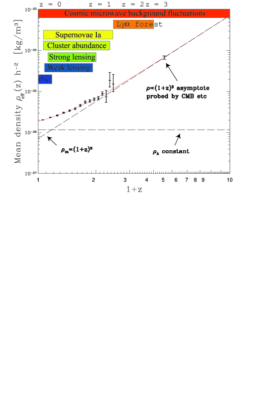
FIG. 1.: Solid curve shows a currently popular model for the evolution of the effective cosmic mean density $\rho_{\rm eff}(z)\propto H(z)^{2}$. This curve uniquely characterizes the spacetime metric to zeroth order. The horizontal bars indicate the rough redshift ranges over which the various cosmological probes discussed are expected to constrain this function. If the Friedmann equation is correct, then $\rho_{\rm eff}(z)=\rho(z)$. Since the redshift scalings of all density contributions except that of dark energy are believed to be straight lines with known slopes in this plot (power laws), combining into a a simple quartic polynomial, an estimate of the dark energy density $\rho_{X}(z)$ can be readily extracted from this curve. Specifically, $\rho\propto(1+z)^{4}$ for the Cosmic Microwave Background (CMB), $\rho\propto(1+z)^{3}$ for nonrelativistic matter (like baryons and CDM), $\rho\propto(1+z)^{2}$ for spatial curvature, $\rho\propto(1+z)^{0}$ for a cosmological constant and $\rho\propto(1+z)^{3(1+w)}$ for quintessence with a constant equation of state $w$. Error bars are for our SNAP SN 1a simulation.

A Parametrizing our ignorance with two functions

There is general consensus that space-time is well described by a metric, at least on non-microscopic scales, so competing theories of gravity differ in their predictions for how the metric evolves with time and responds to the presence of matter. General Relativity (GR) makes specific predictions in the form of the Einstein Field Equations. The parametrized post-Newtonian approximation [50, 51] has been highly successful in describing possible departures from GR in the solar system, and the parametrized post-Keplerian approximation [50, 51] has done the same for for binary orbits, notably binary pulsars. Although GR has so far passed all experimental tests with flying colors, these tests tend to probe only the present epoch. Broad classes of theories have been shown to evolve into GR at late times, so substantial departures from the Einstein field equations are still possible in cosmology.

Assuming merely the cosmological principle (that our position is not special), it follows directly from the observed near-isotropy of the cosmic microwave background (CMB) that the Universe is approximately isotropic and homogeneous. This means that the large-scale metric consists of small perturbations on a Friedman-Robertson-Walker (FRW) background [52]:

$$ds^{2}=dt^{2}-a(t)^{2}\left[{dr\over 1-kr^{2}}-r^{2}d\theta^{2}-\sin^{2}\theta d\phi^{2}\right]$$ (1)

for some function $a(t)$ that describes the expansion history of the Universe. $k=-1$, $0$ or $1$ for an open, flat and closed Universe, respectively. If GR is correct, then $a$ evolves according to the Friedman equation [52]

$$H^{2}\equiv\left({\dot{a}\over a}\right)^{2}={8\pi G\over 3}\rho,$$ (2)

where we define the mean matter density $\rho(z)$ to include a curvature contribution $\rho_{k}\equiv-{3kc^{2}\over 8\pi Ga^{2}}$. Other theories make different predictions. As summarized in Figure 1 and reviewed in the next section, the function $H(z)$ is directly measurable is a variety of ways that make no assumptions about dark matter properties or gravitational field equations, but rely on spacetime geometry alone.

Let us now turn to the evolution of perturbations. The evolution equations are by definition linear to first order, regardless what underlying theory of gravity is being linearized. Assuming that this theory is well approximated by partial differential equations on large scales, these decouple into ordinary differential equations for each Fourier mode, since we are perturbing around a homogeneous metric and derivatives become local in Fourier space. In short, the key observable predicted by theory is the linear growth factor $g(z,k)$, conventionally defined so that a density perturbation $\widehat{\delta}({\bf k})$ with wave vector ${\bf k}$ evolves with redshift as

$$\delta(z,{\bf k})={g(z,k)\over(1+z)}\delta(0;k).$$ (3)

A wide variety of upcoming observations will probe $g(z,k)$, including galaxy and Lyman $\alpha$ forest clustering, the cosmic microwave background, gravitational lensing and type Ia supernovae. When multiple matter components are present, there will of course be one growth factor for each one, whose evolution couple. For photons and neutrinos, the full phase-space distribution is relevant to the dynamics. On large scales, a broad class of models make the simple prediction that $g(z,k)$ is independent of $k$.

B Is matter the matter?

It is obviously premature to guess as to whether upcoming data will favor dark matter or modified gravity. However, it is worth noting that the distinction between these two cases is in fact somewhat blurry. As pointed out by Eddington [53], we can always choose to define matter as that which equals $(8\pi G)^{-1}$ times the Einstein tensor, in which case the Einstein field equations $G_{\mu\nu}=8\pi GT_{\mu\nu}$ become satisfied by definition. This “matter” $T_{\mu\nu}$ would have very strange properties for a generic metric, so the predictive power of GR arises from the fact that observed matter has simple, formalizable properties.

For many modifications of GR, the so defined $T_{\mu\nu}$ is in fact rather regular. Indeed, in the familiar case of adding a cosmological constant, it is largely a matter of taste whether to call it modified gravity or dark energy, corresponding merely to whether we insert it on the left or right hand side of the Einstein equations. In the currently popular class of GR generalizations known as scalar-tensor theories [52, 50, 44], of which Brans-Dicke theory is a special case, we can play the same trick: the Friedman equation (2) remains valid in the conventional (Jordan) frame [44] if we augment the density $\rho$ with the extra “dark energy” term

$$\rho_{x}=\left({1\over\zeta F}-1\right)\rho_{m}+{1\over 8\pi G_{\rm eff}F}\left[U+{Z{\dot{\Phi}}^{2}\over 2}-3H\dot{F}\right],$$ (4)

where the theory is specified by the free functions $F(\Phi)$, $U(\Phi)$ and $Z(\Phi)$ of the dilaton field $\Phi$, $\rho_{m}$ is the density of conventional matter, and

$$\zeta\equiv{G_{\rm eff}\over G_{\rm bare}}={1\over F}\left({2ZF+4(F^{\prime})^{2}\over 2ZF+3(F^{\prime})^{2}}\right)$$ (5)

is the factor by which $G_{\rm eff}$, the effective small-scale Newton’s constant measured in laboratory experiments today, differs from the “bare” one $G_{\rm bare}$ which is truly constant.

As another example, consider a flat toy model where equation (2) is replaced by

$$H^{2}={8\pi G\over 3}{\rho^{2}\over\rho_{*}}$$ (6)

for some constant $\rho_{*}$, i.e., a model where $\rho\propto H$ rather than $\rho\propto H^{2}$. An observer assuming that the Friedman equation equation (2) is valid would then conclude that there is a “dark energy” density $\rho_{x}$ given by

$$\rho_{x}\equiv{3H^{2}\over 8\pi G}-\rho={\rho^{2}\over\rho_{*}}-\rho={\rho_{0}^{2}\over\rho_{*}}(1+z)^{6}-\rho_{0}(1+z)^{3},$$ (7)

a quantity which goes negative for small $\rho$. Here $\rho_{0}$ denotes the current density of baryonic and dark matter.

The modified behavior of linear perturbations in non-GR theories can clearly be attributed to new “matter” as well. Indeed, it has recently been shown [54] that the linearized properties of very general types of dark matter can be conveniently characterized by an effective sound speed and an effective viscosity.

In light of this theory/matter ambiguity, we propose to use the Friedman equation as a definition of an effective mean density

$$\rho_{\rm eff}(z)\equiv{3H(z)^{2}\over 8\pi G_{\rm eff}}.$$ (8)

Thus $\rho_{\rm eff}(z)=\rho(z)$, the true density, if the Friedmann equation is correct. As illustrated in Figure 1, expressing observational results in terms of $\rho_{\rm eff}(z)$ rather than $H(z)$ has the advantage of directly visualizing the dark matter problem. The contribution to $\rho(z)$ from vacuum density is of course constant. Curvature density scales as $(1+z)^{2}$, matter density as $(1+z)^{3}$, radiation density as $(1+z)^{4}$, and a “quintessence”. component with constant equation of state $w$ as $(1+z)^{3(1+w)}$.

A large body of work has been performed during the last few years on constraints and forecasts for more specific models. Cast in our present notation, a particularly useful and popular parametrization of $\rho(z)$ has been [55, 56, 57, 58, 59, 60, 61, 62, 63, 64, 65, 66, 67, 68, 69, 70, 71, 72, 73, 74]

$$\rho(z)=\rho^{0}_{m}(1+z)^{3}+\rho^{0}_{\kappa}(1+z)^{2}+\rho^{0}_{X}(1+z)^{3(1+w)}$$ (9)

for $z\ll 10^{3}$, where $\rho^{0}_{m}$, $\rho^{0}_{\kappa}$ and $\rho_{X}^{0}$ are the present densities of matter, curvature and dark energy, respectively, and the dark energy equation of state $w$ may in turn vary with redshift. In this paper, we treat $\rho_{\rm eff}(z)$ rather than $w(z)$ as the free function for two reasons:

1. It can be estimated from the data without assumptions about gravity (the Einstein field equations) or about the dark energy (which may be out of equilibrium and not have any simple equation of state uniquely determining its pressure from its density).

2. It is more directly related to observed data since, as will be elaborated below, it is given by the first rather than the second derivative of a measured function.

A similar choice was made in [75] as well.

Much progress has also been made on a reconstruction program, aiming to reconstruct the microphysics of specific theories from data. The present work complements this approach, since such reconstructions of, e.g., the quintessence potential [56, 64, 61, 67, 68] or the functions specifying scalar-tensor gravity [43] can be performed with $\rho_{\rm eff}(z)$ and $g(z,k)$ as a starting point.

The rest of this paper is focused on the 0th order function $\rho_{\rm eff}(z)$, with the 1st order function $g(z,k)$ studied in a companion paper [76]. In the next section, we review techniques for measuring $\rho_{\rm eff}(z)$, compute the constraints from current SN 1a data and make forecasts for the proposed SNAP satellite. We discuss our conclusions in Section III.

II Measuring $\rho_{\rm eff}(z)$

The bars at the top of Figure 1 show the redshift ranges over which various types of observations are sensitive to $\rho_{\rm eff}(z)$. We will first review them briefly in turn, then return the SN 1a in greater detail.

A Space-time geometric tests

All cosmological tests based on luminosity, angular size and age (see e.g. [52, 77]) can be described as noisy measurements of some quantities $x_{n}$ at redshifts $z_{n}$, $n=1,...,N$, modeled as

$$x_{n}=a\ln d(z)+b_{n}+\varepsilon_{n},$$ (10)

where $a$ and $b$ are constants independent of $\rho_{\rm eff}(z)$, the function $d$ incorporates the effects of cosmology and $\varepsilon_{n}$ is a random term with zero mean ($\langle\varepsilon_{n}\rangle=0$) including all sources of measurement error. As briefly review below, these observables all probe different weighted averages of the quantity $\rho_{\rm eff}(z)^{-1/2}$.

For luminosity tests like SN Ia, $x_{n}$ is the observed magnitude of the $n^{th}$ object and $d$ is the dimensionless luminosity distance [52]:

$$d_{lum}=(1+z){S(\kappa\eta)\over\kappa},\quad\eta(z)=H_{0}\int_{0}^{z}{dz^{\prime}\over H(z^{\prime})},$$ (11)

where the $\kappa\equiv\sqrt{|1-\Omega_{0}|}$ is the spatial curvature, and $\Omega_{0}\equiv 8\pi G\rho_{\rm eff}(0)/3H^{2}$ is the fraction of critical density contributed by $\rho_{\rm eff}$ today. $S(x)\equiv\sinh x$, $x$ or $\sin x$ when $k=-1$, $0$ or $1$, respectively. From the definition of magnitudes, $a=5/\ln 10$ and $b_{n}=25+5\lg[H_{0}^{-1}c/1{\rm Mpc}]+M_{n}$, where $M_{n}$ is the (hopefully known) absolute magnitude of the $n^{th}$ object. The errors $\varepsilon_{n}$ include errors in extinction correction and intrinsic scatter in the “standard candle” luminosity.

For tests involving the observed angular sizes $\theta_{n}$ of objects at redshifts $z_{1},...,z_{N}$ with (hopefully known) linear sizes $D_{1},...,D_{N}$, we can take $d$ to be the dimensionless angular size distance [52]: $d_{ang}=d_{lum}/(1+z)^{2}$. This gives $x_{n}\equiv\ln\theta_{n}$ (angles measured in radians), $a\equiv=-1$ and $b_{n}\equiv\ln[H_{0}D_{n}/c]$. For such tests (e.g. [78, 79]), $\varepsilon_{n}$ includes scatter in the “standard yardstick” size.

For tests involving estimates $t_{n}$ of the age of the Universe at redshifts $z_{n}$, we define $x_{n}\equiv\ln H_{0}t_{n}$. Setting $a=1$ and $b_{n}=0$, this gives [52]

$$d_{age}=H_{0}\int_{z}^{\infty}{dz^{\prime}\over(1+z^{\prime})H(z^{\prime})}.$$ (12)

Equation (10) implicitly assumes that the the measurement errors $\varepsilon_{n}$ for $x_{n}$ are additive. This is a popular approximation in many cases, notably for luminosity distance where the actual measurement is a magnitude proportional to $\ln d$, and tends to be accurate if the relative error (on flux, angular size, age, etc.) is small ($\ll 1$). In other cases, a more appropriate error model should be employed.

Ideally, we would like to measure the function $\rho_{\rm eff}(z)$ in ways that are sensitive only to the global spacetime geometry and do not depend on $g(z,k)$. The measurements that come closest to this ideal are arguably those involving the brightness, angular size and age of distant objects, in situations where the calibration of the “standard candle”, “standard ruler” or “standard clock” depends mainly on microphysics. However, great care must be taken when constraining competing theories of gravity etc. (as opposed to more mundane dark energy), since slight time variations in microphysical constants could affect the standard calibrators and masquerade as modifications to $\rho_{\rm eff}(z)$. For instance, time-variation in a non-gravitational “constant” (say the fine-structure constant “alpha”) could alter the intrinsic energetics and time-evolution of a supernova explosion, making it a bad standard candle. If such an effect were present but neglected, then we would draw an incorrect conclusion about the luminosity distance to the supernova and consequently also about the cosmic geometry.

Terrestrial constraints are are now so strong that time-variation of the fine structure constant $\alpha$ is unlikely to cause such misinterpretations: variations in $\alpha$ are limited to around a part per million over cosmological timescales [80] (c.f. [81]). A more serious concern in this context is time variations in the effective gravitational constant, expected in many scalar-tensor theories according to equation (5). Here the observational constraints are weaker, permitting variations of a few percent over cosmological time scales [82, 83], which could among other things cause distant supernovae to be systematically brighter or fainter than nearby ones.

As Figure 1 indicates, the function $\rho_{\rm eff}(z)$ is probed by the growth of clustering as well, via the power spectrum growth in the Ly$\alpha$ forest, weak lensing and galaxy surveys as well as via the abundance evolution of galaxy clusters and lensing systems. However, these probes all depend on the function $g(z,k)$ as well, i.e., on the next order of perturbation theory. The Alcock-Paczynski test elegantly eliminates the dependence on $g(z,k)$ caused by number density evolution, but involves certain bias-related issues [84, 85, 61].

Although the CMB power spectrum $C_{\l}$ depends on the growth $g$, the effect is “vertical” rather than “horizontal”. In other words, as long as some detectable acoustic peak structure is visibly preserved, it should be possible to extract the angular scale corresponding to the horizon size at recombination fairly independently of $g$. With additional knowledge of the dark matter density, this provides a clean measurement of $d_{lum}$ at $z\sim 10^{3}$.

If GR is correct so that $g$ and the vertical structure of the acoustic peak heights can be computed from first principles, then the CMB is a sensitive probe of the high-redshift asymptote in of the $\rho_{\rm eff}$ curve in Figure 2, where the Universe becomes matter dominated. Writing $\rho_{m}(z)=\rho_{m}^{0}(1+z)^{3}$, the MAP and Planck satellites are expected to measure $\rho_{m}^{0}$ to accuracies of $10\%$ and $1\%$, respectively. However, in contrast to, e.g., SN 1a, the CMB is mainly sensitive to the physical matter density $\rho_{m}$, not to the plotted quantity $\rho_{m}/h^{2}$, since this is what matters for the acoustic oscillations at $z>10^{3}$. The ultimate accuracy with which we can measure $\rho_{m}^{0}/h^{2}$ (equivalently $\Omega_{m}$) is therefore likely to be limited not by CMB issues but by our ability to measure $h$, either directly or by combining various complementary measurements [86].

B $\rho_{\rm eff}(z)$ from existing SN 1a data

Of the various low-redshift probes of $\rho_{\rm eff}(z)$ that we discussed, type 1a supernovae are arguably the most sensitive at the present time. We will therefore compute constraints on $\rho_{\rm eff}(z)$ from current SN 1a data and make forecasts for the accuracy attainable with future measurements.

Figure 2 shows the measured luminosity distance for 92 SN 1a, combining the high redshift sample of 42 from [87] with the 50 reported in [88] with the MLCS method. Apart from systematic and calibration issues, our desired function $\rho_{\rm eff}(z)$ is simply given by the derivative of the curve around which they scatter: $\rho_{\rm eff}(z)=3H_{0}^{2}/8\pi G_{\rm eff}\eta^{\prime}(z)^{2}\propto h^{2}/\eta^{\prime}(z)^{2}$. Since the slope is seen to fall, the cosmic density clearly increases at high redshift. If standard GR is correct ($\rho_{\rm eff}=\rho$), then this fact that $d\rho_{\rm eff}/dz>0$ corresponds to the weak energy condition [92, 75] that the density measured by any observer is non-negative, and is equivalent to the pressure-to-density ratio constraint $p/\rho\geq-1$. A more detailed reconstruction of $\rho(z)$ is shown in Figure 3, and was computed by fitting a homogeneous quartic polynomial (dashed curve in Figure 2) to $\eta(z)$. Using the notation of equation (10), the fit was done by minimizing

$$\chi^{2}=\sum_{n=1}^{n}\left({x_{n}-a\ln d(z_{n})-b_{n}\over\sigma_{n}}\right)^{2},$$ (13)

where $\sigma_{n}$ are the quoted 1 sigma magnitude errors [87, 88]. This gives the fitting parameters (polynomial coefficients) as linear combinations of the data $x_{n}$. The 1 sigma errors in Figure 3 are obtained by propagating the errors on these fitting parameters. The figure clearly illustrates the familiar fact that dark energy/modified gravity is required: the slope of the $\rho_{\rm eff}(z)$-curve is too shallow at low redshift to be explainable in terms of ordinary matter $(\rho\propto[1+z]^{3}$), spatial curvature $(\rho\propto[1+z]^{2}$) or some combination of the two.

Since $\rho_{\rm eff}(z)\propto h^{2}/\eta^{\prime}(z)^{2}$, the SN 1a give us a direct measurement of $\rho_{\rm eff}(z)/h^{2}$, where $h$ is the Hubble parameter today in units of 100 km/s/Mpc. Changing $h$ thus shifts $\rho_{\rm eff}$ vertically on a logarithmic plot like Figure 2 without affecting its problematic slope.

To assess the sensitivity of our results to method details, we show alternative analyses in figures 4 and 5. Here we replaced the polynominal fitting function by piecewise quadratic and piecewise linear interpolating functions for $\eta(z)$, respectively. For the quadratic case, we enforced that the function have continuous derivative, thereby making $\rho_{\rm eff}$ a continuous function. The results are seen to be quite robust, in all cases agreeing well with the “concordance” model and indicating a shallow slope at low redshifts incompatible with just matter and curvature alone. A very nice non-parametric SN 1a analysis was recently performed by Wang & Garnavich [75], and it is interesting to compare the two studies since they were performed concurrently and independently. The quantitative agreement is good taking into account that [75] treat the dark energy density $\rho(z)-\rho_{m}^{0}(1+z)^{3}$ rather than $\rho_{\rm eff}(z)$ as the free function and marginalize over $\rho_{m}$ imposing the weak energy condition. The SN 1a data thus speak loud and clear: the dark energy puzzle is robust to theoretical assumptions and method details.

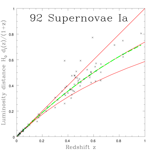
FIG. 2.: Crosses show the luminosity distance for 92 SN 1a. From top to bottom, solid curves correspond to models $(\Omega_{\rm m},\Omega_{\Lambda})=(0,1)$, $(0.38,0.62)$ and $(1,0)$, respectively. The middle curve is almost indistinguishable from the best fit quartic polynomial (dashed). The density history $\rho_{\rm eff}(z)$ is simply the squared inverse slope of this curve. Scatter increases with $z$ since the relative distance errors are roughly constant.

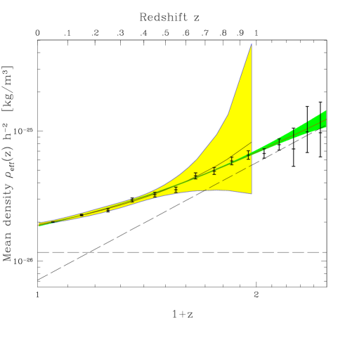
FIG. 3.: Zoom of Figure 1 showing constraints on $\rho_{\rm eff}(z)$ from actual and simulated data, assuming a flat Universe. Solid black curve shows best fit to the 92 SN1a, corresponding to the polynomial fit shown in Figure 2, and yellow/light grey area shows the associated 68% confidence region. Green/dark grey area shows the corresponding 68% confidence region from our SNAP simulation, for a fiducial model with $\Omega_{\rm m}=0.38$, $\Omega_{\Lambda}=0.62$ (red/grey curve) whose two components are shown as dashed lines. Error bars are for the non-parametric reconstruction of Section II C, spaced so that measurements of neighboring bands are uncorrelated, and are identical to those shown in Figure 1.

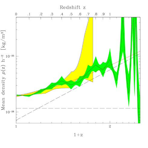
FIG. 4.: Same as previous figure, but using a quadratic spline instead of a polynomial to fit $\eta(z)$. Bin widths were $\Delta z=0.2$ for the actual data and $\Delta z=0.1$ for SNAP.

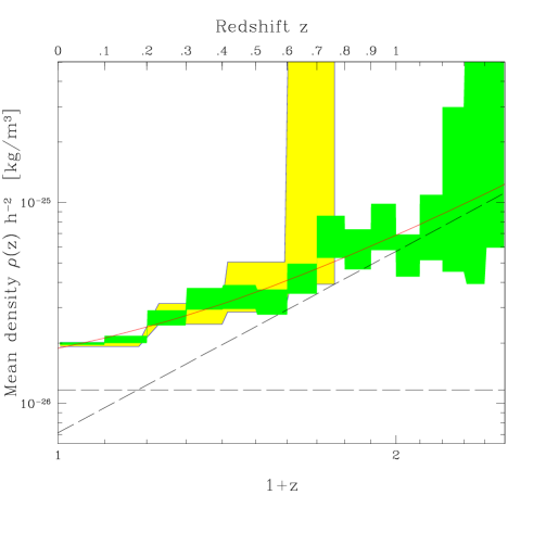
FIG. 5.: Same as previous figure but using linear interpolation to fit $\eta(z)$, giving a piecewise constant density.

C With upcoming SN 1a data

The proposed SNAP satellite would measure of order $N=2000$ SN 1a out to redshifts around 1.2 or higher [61]. There has been substantial debate in the literature about the accuracy with which the equation of state can be reconstructed [60, 61, 64, 66, 67, 68, 69, 70, 71, 72, 73, 74, 75]. We will now compute how accurately SNAP can measure $\rho_{\rm eff}(z)$. It is straightforward to do this numerically in a “black box” fashion, and figures 3-5 show the result of doing this with simulations in the same way as we did it for the currently existing data. However, because of the strong interest and substantial resources focused on designing such future probes, it is also worthwhile to gain intuition on how experimental specifications translate into model constraints. We will therefore derive an analytic result which has the advantage of explicitly showing how the results scale when changing survey specifications, the smoothing scale, etc.

1 An analytic error formula

Defining $f(z)\equiv H(0)/H(z)$, we have $\eta(z)=\int_{0}^{z}f(z^{\prime})dz^{\prime}$ and wish to know how accurately $f$ can be recovered from noisy measurements of $\eta$. In other words, we simply want to compute the derivative of a function measured with sparse sampling and noise. The errors on $\rho_{\rm eff}(z)\propto 1/f(z)^{2}$ then follow trivially from those on $f(z)$.

The accuracy with which $f(z)$ can be measured is readily computed with the Fisher information matrix formalism [93, 94] with infinitely many parameters to be estimated (the value of $f$ at each $z$). The amount of information about these parameters in the SN 1a data is given by [90]

$${\bf F}(z^{\prime},z^{\prime\prime})={a^{2}N\over(\Delta m)^{2}}\int_{0}^{\infty}g(z)w_{z^{\prime}}(z)w_{z^{\prime\prime}}(z)dz,$$ (14)

where $a\equiv 5/\ln 10$, $\Delta m$ is the rms SN 1a magnitude error, $N$ is the number of supernovae, $g(z)$ is their redshift distribution (normalized to integrate to unity), and

$$w_{z^{\prime}}(z)\equiv{\partial\ln\eta(z)\over\partial f(z^{\prime})}={\theta(z-z^{\prime})\over\eta(z)}.$$ (15)

since $\eta^{\prime}(z)=f(z)$. Here $\theta$ denotes the Heaviside step function ($\theta(z)=1$ for $z\geq 0$, vanishing otherwise). Equation (14) thus gives

$${\bf F}(z,z^{\prime}) = \int\theta(z^{\prime\prime}-z)\theta(z^{\prime\prime}-z^{\prime})h(z^{\prime\prime})^{-1}dz^{\prime\prime}$$ (16)

$$= \int_{{\rm max}(z,z^{\prime})}^{\infty}h(z^{\prime\prime})^{-1}dz^{\prime\prime},\quad\hbox{where}$$ (17)

$$h(z) \equiv {(\Delta m)^{2}\over a^{2}N}{\eta(z)^{2}\over g(z)}.$$ (18)

The covariance matrix ${\bf C}$ giving the best attainable error bars on our estimated parameters is the inverse of this infinite-dimensional matrix, ${\bf C}={\bf F}^{-1}$. Fortunately, this inverse can be computed analytically, giving

$${\bf C}(z,z^{\prime})=-h^{\prime}(z)\delta^{\prime}(z-z^{\prime})-h(z)\delta^{\prime\prime}(z-z^{\prime}),$$ (19)

where $\delta$ denotes the Dirac delta function. This follows from the identity

$$\int{\bf C}(z,z^{\prime\prime}){\bf F}(z^{\prime\prime},z^{\prime})dz^{\prime\prime}=\delta(z-z^{\prime}),$$ (20)

which is proven by substituting equations (16) and (19), integrating by parts twice and using that $\theta^{\prime}(x)=\delta(x)$. In practice we obviously want to smooth our estimated $f$-function (${\tilde{f}}(z)$, say) to reduce noise. Using weighted averages ${\tilde{f}}_{i}\equiv\int\psi_{i}(z){\tilde{f}}(z)dz$, the covariance matrix ${\bf C}_{ij}$ for these averages is

$$\int{\bf C}(z,z^{\prime})\psi_{i}(z)\psi_{j}(z^{\prime})dzdz^{\prime}=\int h(z)\psi^{\prime}_{i}(z)\psi^{\prime}_{j}(z)dz,$$ (21)

employing equation (19) and integrating by parts. Once these errors on $f(z)$ have been computed, it is of course trivial to map them into errors on $\rho_{\rm eff}(z)$. When the relative errors are small $(\Delta f\ll f)$, we have simply $\Delta\rho_{\rm eff}/\rho_{\rm eff}\approx\Delta f/f$.

2 Smoothing functions

Using Gaussian smoothing functions

$$\psi_{i}(z)\equiv{1\over(2\pi)^{1/2}\Delta z}e^{-{1\over 2}\left({z-z_{i}\over\Delta z}\right)^{2}},$$ (22)

the error bars $\Delta f_{i}\equiv{\bf C}_{ii}^{1/2}$ are given by

$$\Delta f_{i}\approx{\ln 10\over 10\pi^{1/4}}{\Delta m\,\eta(z_{i})\over(\Delta z)^{3/2}N^{1/2}g(z_{i})^{1/2}}$$ (23)

for the case where the smoothing scale $\Delta z$ is much smaller than the scale on which $\eta$ and $g$ vary substantially. In the same approximation, the dimensionless correlation coefficients between the different averages are

$$r_{ij}\approx(2-n^{2})e^{-n^{2}},\quad\hbox{where}\quad n\equiv\left({z_{i}-z_{j}\over\Delta_{z}}\right)$$ (24)

is the number of smoothing lengths by which the two redshifts are separated, so neighboring measurements are uncorrelated if they are separated by $\sqrt{2}\Delta z$. Another interesting case for our discussion below is that of “triangular” smoothing functions

$$\psi_{i}(z)=\cases{{\Delta z-|z-z_{i}|\over\Delta z}&if $|z-z_{i}|<\Delta z$,\cr\vskip 4.0pt\cr 0&otherwise,}$$ (25)

which gives

$$\Delta f_{i}\approx{\sqrt{2}\ln 10\over 5}{\Delta m\,\eta(z_{i})\over(\Delta z)^{3/2}N^{1/2}g(z_{i})^{1/2}}$$ (26)

in the same approximation. Here there are strong anticorrelations $r=-2^{-1/2}\approx-0.7$ between neighboring bins, and all longer-range correlations vanish. “Boxchar” smoothing where we simply average in bins, $\psi(z)=\theta(\Delta z/2-|z-z_{i}|)/\Delta z$, may seem like a natural choice. This is a disaster, however, since the resulting $\delta$-functions in $\psi^{\prime}_{i}$ blow up when squared. This problem is easy to understand physically. In a toy example where we have many SN 1a equispaced in redshift and estimate $\eta^{\prime}(z)$ by simply differencing neighboring supernovae, averaging a segment of these derivative estimates will reduce to simply differencing the first and the last, placing all the statistical weight on merely two objects.

As we will return to below, our black-box numerical method can also understood in terms of smoothing functions of a particular form.

The exact result of equation (21) and the approximation of equation (23) illustrate a number of issues relevant to measuring $\rho_{\rm eff}(z)$ in practice, as discusses in the following subsections.

3 Redshift resolution

Errors scale as $(\Delta z)^{-3/2}$ rather than $(\Delta z)^{-1/2}$ because of the derivative nature of what we are measuring, which means that very large number of SN 1a are needed to probe the small-scale structure of $\rho_{\rm eff}(z)$. It also means that care must be taken in interpreting error forecasts to avoid coming away with a misleadingly pessimistic impression. The superiority of SNAP over existing data is partly hidden in figures 4 and figures 5 since $\Delta z$ is halved for SNAP, roughly tripling error bars. The error bars from the numerical SNAP simulations in figures 4 and figures 5 agree well with the analytic ones of equation (25) with $\Delta z=0.1$ as well as those of [75], but are substantially larger than those from the polynomial fit shown in Figure 3. This is because the quartic polynomial enforces more smoothness, effectively increasing $\Delta z$. The non-parametric error bars in Figure 3 from equation (23) using Gaussian smoothing are a factor of $2^{3/2}\pi^{1/4}\sim 4$ smaller than those from equation (26) using triangle smoothing, which is related to the fact that the triangle smoothing functions have standard deviations $\sqrt{6}$ times narrower than the Gaussian ones.

Which error bars are most appropriate depends on what the data are to be used for. Constraining models where $\rho_{\rm eff}$ may change abruptly with $z$ requires high redshift resolution and associated large error bars like in fugures 4 and 5. Most published models, however, predict rather smooth functions $\rho_{\rm eff}(z)$, so the small error bars from a low-order polynomial fit like in Figure 3 give the most accurate representation of how well SNAP could distinguish them from one another.

4 High-$z$ sensitivity

Since errors scale as $\eta(z)$, one does worse at large $z$. However, since $\eta(z)$ flattens out around $z\sim 1$ and asymptotes to a constant as $z\to\infty$, this is not a fundamental limitation to probing very large redshifts — the challenge is simply to find suitable high-$z$ standard candles or other reference objects to prevent $g(z)$ from going to zero in the denominator.

5 Optimal estimation

Equation (21) also indicates what the optimal estimator is for non-parametric measurement of $\rho_{\rm eff}(z)$. It is easy to verify that when the smoothing scale $\Delta z$ is much smaller than the scale $h/|h^{\prime}|$ on which $h$ varies substantially, weighting the actual data with the function $\psi_{i}^{\prime}(z)h(z)$ and normalizing appropriately will recover the minimal Fisher matrix error bars. In practice, $g(z)$ is of course not a smooth function but a sum of $\delta$-functions at the observed SN 1a redshifts, so an additional correction for the non-even spacing between adjacent SN 1a is necessary.

The black box of $\chi^{2}$-minimization can also be understood in terms of smoothing functions and equation (21). Since $\chi^{2}$ depends quadratically on the free parameters, the best fit parameters and hence also the recovered function ${\tilde{f}}(z)$ depends linearly on the observed $\eta$-values for each supernova, once the redshifts are given. In other words, we can write

$${\tilde{f}}_{i}=\sum_{j=1}^{N}\psi^{\prime}_{i}(z_{j})\eta_{j}$$ (27)

for some function $\psi_{i}$, where $\eta_{j}$ is the observed $\eta$-value for the $j^{th}$ supernova. In an attempt to demystify the numerical results somewhat, we have plotted these weight functions $\psi^{\prime}_{i}$ in Figure 6 for estimating $f(z)$ with SNAP at $z\sim 0.8$. We see that for both the quadratic spline and the linear interpolation cases, there is substantial ringing. Moreover, the measurement of $\eta^{\prime}(0.8)$ is seen to involve supernovae over a very broad range of redshifts, not merely near $z=0.8$. In contrast, the triangle smoothing function would be more local, giving $\psi^{\prime}(z)=-1$ for $z=0.7-0.8$, $\psi^{\prime}(z)=1$ for $z=0.8-0.9$ and zero elsewhere, simply estimating the derivative $\eta^{\prime}(0.8)$ by subtracting measurements to the left from ones to the right. The Gaussian smoothing function behaves similarly, merely with less abrupt behavior. Just as sophisticated data analysis techniques developed by numerous groups have enhanced the science return of recent CMB missions, there may well be room for methodological improvement here. For instance, what is a good parametrization of $f$ that leads to compact, easy-to-interpret weight functions?

FIG. 6.: Sample weight functions $\psi^{\prime}(z)$ extracted from the $\chi^{2}$-minimization are plotted for the quadratic spline (dashed) and linear interpolation (solid), both probing the derivative $\eta^{\prime}(z)$ at $z\sim 0.8$. Excessive ringing drives up the error bars and the fact that the functions are so wide complicates the interpretation.

III DISCUSSION

We have argued that the effective density evolution $\rho_{\rm eff}(z)$ and the linear growth factor $g(z,k)$ constitute the natural meeting point for theory to confront observation in terms of linear cosmology, since they can be measured with very few assumptions about unseen matter and the underlying theory of gravity. This generalizes studies of the equation of state $w$.

We analyzed current SN 1a data in this framework, and showed that the statistical constraints on $\rho_{\rm eff}(z)$ are already fairly strong for $z\mathrel{\hbox to0.0pt{\lower 3.0pt\hbox{$\mathchar 536\relax$}\hss}\raise 2.0pt\hbox{$\mathchar 316\relax$}}0.5$. This alternative approach confirms the results of previous SN 1a analyses [88, 87, 89, 75], and provides a clean and model-independent case for either dark energy or modified gravity, since $\rho_{\rm eff}(z)$ has the wrong logarithmic slope at low redshift to be explained by either matter (slope $-3$) or spatial curvature (slope $-2$).

We estimated the accuracy with which the proposed SNAP satellite should be able to measure $\rho_{\rm eff}(z)$, both with a numerical simulation involving polynomial fitting and by deriving a non-parametric analytic formula, and found that precision density measurements should be attainable in about a dozen independent redshift bins out to $z\sim 1.2$. Since errors grow as $(\Delta z)^{-3/2}$ as the bin width $\Delta z$ is reduced, the large numbers of SN 1a of SNAP are absolutely necessary to resolve the small-scale structure of $\rho_{\rm eff}(z)$. The reason that $w(z)$ is so much harder to constrain accurately is that it involves a second derivative of the data, causing error bars to blow up as $(\Delta z)^{-5/2}$.

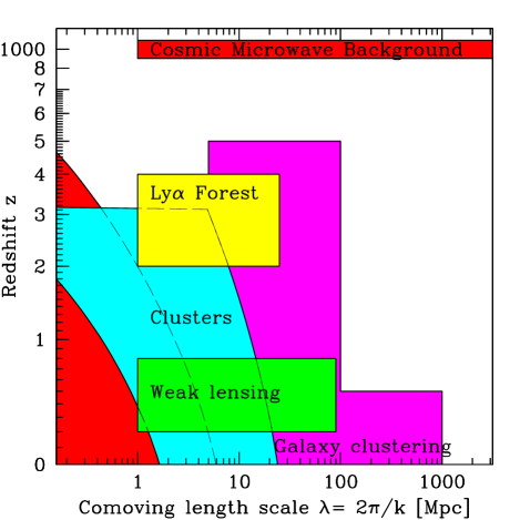
FIG. 7.: Shaded regions show crude estimates of the ranges of scale and redshift over which various observations are likely to probe the growth factor $g(k,z)$ over the next few years. The lower left region, delimited by the dashed line, is the non-linear regime where rms density fluctuations exceed unity for the “concordance” model from [9].

We focused on the 0th order function $\rho_{\rm eff}(z)$, with the 1st order function $g(z,k)$ studied in detail in a companion paper [76]. To place our discussion in its observational context, Figure 7 shows the rough ranges of scale and redshift over which various observations are likely to probe $g(k,z)$ over the next few years. Regardless of what detailed assumptions are made, it is clear from figures 1 and 7 that upcoming measurements of the CMB, the Ly$\alpha$ Forest, weak lensing, cluster abundance and galaxy clustering have the potential to probe both functions back to high redshift over several orders of magnitude in scale, allowing numerous consistency checks between different types of measurements. Measuring $g(z)$ for pressureless matter could provide an independent determination of $H(z)$ [56].

It may be possible to extract further constraints on dark energy/modified gravity from going to higher order in perturbation theory or studying the nonlinear regime. Such nonlinear issues were indeed the motivation for some recent suggestions for dark matter and modified gravity [39, 40, 42]. Although many proposed quintessence fields do not cluster on small scales, early work in this direction [44, 45] has discussed how temporal and perhaps spatial variations in Newton’s constant may be an observable signature.

In conclusion, the evidence for dark energy/modified gravity has emerged as one of the key puzzles of modern cosmology. Fortunately, there are at least half a dozen observational approaches that can directly probe the time-evolution of the effective mean density and clustering, so by going after this problem with the full arsenal, there is real hope that the cosmology community can resolve it over the next decade.

The author wishes to thank Arthur Kosowsky and Jim Peebles for provocative questions triggering this work, and Bernd Brügman, Angélica de Oliveira-Costa, Daniel Eisenstein, Gilles Esposito-Farese, Wayne Hu, Dragan Huterer, Arthur Kosowsky, David Polarski, Alexei Starobinski, Paul Steinhardt, Mike Turner and Robert Wald for helpful comments.

Support for this work was provided by NSF grant AST00-71213, NASA grant NAG5-9194 and the University of Pennsylvania Research Foundation.

REFERENCES

- [1] A. E. Lange et al., Phys. Rev. D 63, 042001 (2001).
- [2] M. Tegmark and M. Zaldarriaga, Phys. Rev. Lett. 85, 2240 (2000).
- [3] A. Balbi et al., ApJL 545, L1 (2000).
- [4] S. L. Bridle et al., MNRAS 321, 333 (2001).
- [5] W. Hu, M. Fukugita, M. Zaldarriaga and, M. Tegmark, ApJ 549, 669 (2001).
- [6] A. Jaffe et al., Phys. Rev. Lett. 86, 3475 (2000).
- [7] W. H. Kinney, A. Melchiorri and, A. Riotto, Phys. Rev. D 63, 23505 (2001).
- [8] R. Durrer and B. Novosyadlyj, MNRAS 324, 560 (2001).
- [9] M. Tegmark, M. Zaldarriaga and, A. J. S. Hamilton, Phys. Rev. D 63, 43007 (2001).
- [10] X. Wang, M. Tegmark and, M. Zaldarriaga, Phys. Rev. D 65, 123001 (2002).
- [11] G. Efstathiou et al., MNRAS 330L, 29 (2002). ,
- [12] K. Scholberg et al., hep-ex/9905016 (1999).
- [13] M. E. Carlson, M. E. Machacek and, L. J. Hall, ApJ 398, 43 (1992).
- [14] A. A. de Laix, R. J. Scherrer and, R. K. Schaefer, ApJ 452, 495 (1995).
- [15] D. N. Spergel and P. J. Steinhardt, Phys. Rev. Lett. 84, 3760 (2000).
- [16] C. J. Hogan and J. J. Dalcanton, Phys. Rev. D 62, 063511 (2000).
- [17] S. Hannestad and R. J. Scherrer, Phys. Rev. D 62, 043522 (2000).
- [18] A. Burkert, ApJL 534, L143 (2000).
- [19] C. Firmani, E. D’Onghia, V. Avila-Reese, G. Chincarini and, X. Hernández, MNRAS 315, L29 (2000).
- [20] H. J. Mo and S. Mao, MNRAS 318, 163 (2000).
- [21] C. S. Kochanek and M. White, ApJ 543, 514 (2000).
- [22] N. Yoshida, V. Springel and, S. D. M. White, ApJL 544, L87 (2000).
- [23] M. Kaplinghat, L. Knox and, M. S. Turner, Phys. Rev. Lett. 85, 3335 (2000).
- [24] S. A. Bonometto and R. Valdarnini, ApJL 299, L71 (1985).
- [25] R. Schaeffer and J. Silk, ApJ 332, 1 (1988).
- [26] S. Colombi, S. Dodelson and, L. M. Widrow, ApJ 458, 1 (1996).
- [27] P. Colín, V. Avila-Reese and, O. Valenzuela, ApJ 542, 622 (2000).
- [28] V. K. Narayanan, D. N. Spergel, R. Davé and, C. P. Ma, ApJL 543, L103 (2000).
- [29] P. Bode, J. P. Ostriker and, N. Turok, ApJ 556, 93 (2001).
- [30] W. Hu, R. Barkana and, Gruzinov A, Phys. Rev. Lett. 85, 1158 (2000).
- [31] P. J. E. Peebles, ApJL 534, 127 (2000).
- [32] I. Zlatev, L. Wang and, P. J. Steinhardt, Phys. Rev. Lett. 82, 896 (1999).
- [33] A. Sahni and A. A. Starobinsky, Int. J. Mod. Phys. D 4, 373 (2000).
- [34] P. J. E. Peebles, astro-ph/9910234 (1999).
- [35] P. J. E. Peebles, astro-ph/0011252 (2000).
- [36] J. A. Sellwood and A. Kosowsky, astro-ph/0009074 (2000).
- [37] M. J. Disney, Gen. Rev. & Grav. 32, 1125 (2000).
- [38] S. S. McGaugh, ApJL 541, L33 (2000).
- [39] M. Milgrom, ApJ 270, 365 (1983).
- [40] M. Milgrom, astro-ph/9810302 (1998).
- [41] T. Damour, gr-qc/9904057 (1999).
- [42] P. Mannheim, Found. Phys. 30, 709 (2000).
- [43] B. Boisseau, G. Esposito-Farèse, D. Polarski and, A. A. Starobinsky, Phys. Rev. Lett. 85, 2236 (2000).
- [44] G. Esposito-Farèse and D. Polarski, Phys. Rev. D 63, 063504 (2001).
- [45] E. Gaztañaga and A. Lobo, ApJ 548, 47 (2001).
- [46] P. Binetruy and J. Silk, Phys. Rev. Lett. 87, 031102 (2001).
- [47] J. Uzan P and F. Bernardeu, Phys.Rev. D 64, 083004 (2001).
- [48] J. Hwang and H. Noh, Phys. Rev. D 65, 023512 (2002).
- [49] D. Behnke, D. Blaschke, V. N. Pervushin and, D. Proskurin, Phys. Lett. B 530, 20 (2002).
- [50] C. M. Will, Theory and Experiment in Gravitational Physics (Cambridge, Cambridge University Press, 1993).
- [51] C. M. Will, gr-qc/9811036 (1998).
- [52] S. Weinberg, Gravitation and Cosmology (New York, Wiley, 1972).
- [53] A. Eddington, Space, Time & Gravitation (Cambridge, Cambridge University Press, 1920).
- [54] W. Hu, ApJ 506, 485 (1998).
- [55] P. M. Garnavich et al., ApJ 509, 74 (1998).
- [56] A. A. Starobinsky, JETP Lett. 68, 757 (1998).
- [57] G. Efstathiou, MNRAS 310, 842 (1999).
- [58] S. Perlmutter, M. S. Turner and, M. White, Phys. Rev. Lett. 83, 670 (1999).
- [59] A. R. Cooray and D. Huterer, ApJL 513, L95 (1999).
- [60] D. Huterer and M. S. Turner, Phys. Rev. D 60, 081301 (1999).
- [61] D. Huterer and M. S. Turner, 64;123527 (2001).
- [62] J. A. Newman, ApJL 534, L11 (2000).
- [63] J. A. S. Lima and J. S. Alcaniz, MNRAS 317, 893 (2000).
- [64] T. D. Saini, S. Raychaudhury, V. Sahni and, A. A. Starobinsky, Phys. Rev. Lett. 85, 1162 (2000).
- [65] R. Bean and A. Melchiorri, PRD 65, 041302 (2001).
- [66] J. Kujat, Linn A M, R. J. Scherrer and, Weinberg D H, ApJ 572, 1-14 (2001).
- [67] I. Maor, R. Brustein and, P. J. Steinhardt, PRL 86, 6 (2002).
- [68] I. Maor, R. Brustein, J. McMahon and, P. J. Steinhardt, PRD 65, 123003 (2002).
- [69] J. Weller and A. Albrecht, PRD 65, 103512 (2002).
- [70] I. Wasserman, astro-ph/0203137 (2002).
- [71] D. N. Spergel and G. D. Starkman, astro-ph/0204089 (2002).
- [72] P. J. E. Peebles and B. Ratra, astro-ph/0207347 (2002).
- [73] J. A. Frieman, D. Huterer, E. V. Linder and, M. S. Turner, astro-ph/0208100 (2002).
- [74] E. V. Linder and D. Huterer, astro-ph/0208138 (2002).
- [75] Y. Wang and P. M. Garnavich, ApJ 552, 445 (2001).
- [76] M. Tegmark and M. Zaldarriaga, astro-ph/0207047 (2002).
- [77] P. J. E. Peebles, Principles of Physical Cosmology (Princeton, Princeton University Press, 1993).
- [78] E. J. Guerra, R. Daly and, L. Wan, ApJ 544, 659 (2000).
- [79] U. Pen, New. Astr. 2, 309 (1997).
- [80] T. Damour and F. Dyson, Nucl. Phys. B 480, 37 (1996).
- [81] J. K. Webb, V. V. Flambaum, C. W. Churchill, M. J. Drinkwater and, J. D. Barrow, Phys. Rev. Lett. 82, 884 (1999).
- [82] J. O. Dickey et al., Science 265, 482 (1994).
- [83] J. G. Williams, X. X. Newhall and, J. O. Dickey, Phys. Rev. D 53, 6730 (1996).
- [84] C. Alcock and B. Paczynski, Nature 281, 358 (1979).
- [85] V. Nair, ApJ 522, 569 (1999).
- [86] D. J. Eisenstein, W. Hu and, Tegmark M, ApJ 518, 2 (1999).
- [87] S. Perlmutter et al., Nature 391, 51 (1998).
- [88] A. G. Riess et al., Astron. J. 116, 1009 (1998).
- [89] M. White, ApJ 506, 495 (1998).
- [90] M. Tegmark, D. J. Eisenstein, W. Hu and, R. Kron, astro-ph/9805117 (1998).
- [91] G. Huey, L. Wang, R. Dave, R. R. Caldwell and, P. J. Steinhardt, Phys. Rev. D 59, 063005 (1999).
- [92] R. M. Wald, General Relativity (Chicago, University of Chicago Press, 1984).
- [93] R. A. Fisher, J. Roy. Stat. Soc. 98, 39 (1935).
- [94] M. Tegmark, A. N. Taylor and, A. F. Heavens, ApJ 480, 22 (1997).