The ultraviolet visibility and quantitative morphology of galactic disks at low and high redshift

Abstract

We have used ultraviolet (200 nm) images of the local spiral galaxies M33, M51, M81, M100, M101 to compute morphological parameters of galactic disks at this wavelength : half-light radius $r_{hl}$, surface brightness distributions, asymmetries ($A$) and concentrations ($C_{A}$). The visibility and the evolution of the morphological parameters are studied as a function of the redshift. The main results are : local spiral galaxies would be hardly observed and classified if projected at high redshifts (z $\geq$ 1) unless a strong luminosity evolution is assumed. Consequently, the non-detection of large galactic disks cannot be used without caution as a constraint on the evolution of galatic disks. Spiral galaxies observed in ultraviolet appear more irregular since the contribution from the young stellar population becomes predominent. When these galaxies are put in a (log $A$ vs. log $C_{A}$) diagram, they move to the irregular sector defined at visible wavelengths. Moreover, the log $A$ parameter is degenerate and cannot be used for an efficient classification of morphological ultraviolet types. The analysis of high redshift galaxies cannot be carried out in a reliable way so far and a multi-wavelength approach is required if one does not want to misinterpret the data.

1 Introduction

At large distances, very concentrated galaxies with large surface brightnesses are more easily observed. It is generally accepted that these galaxies are probably spheroids (Steidel et al. Steidel96 (1996), Giavalisco et al. 1996b ). The detection of spirals and, more generally, galactic disks which exhibit a lower surface brightness is far more difficult. Moreover, at high z we observe the rest frame ultraviolet (UV) emission of galaxies redshifted in the visible. If we wish to compare high redshift objects with local ones, we must account for this effect by choosing templates observed in the appropriate wavelength range. The morphology of moderate and high z galaxies has been intensively studied lately (Abraham et al. 1996a ; Abraham et al. 1996b ; Schade et al. Schade96 (1996); Lilly et al. Lilly98 (1998)) and structural parameters have been proposed which can be measured in a rather automatic way (Abraham et al. 1996a ). These parameters are quantities like the half-light radius ($r_{hl}$) or the mean surface brightness but also more sophisticated quantities such as the concentration (C_A) or the asymmetry ($A$). Before being applied to distant galaxies these parameters must be calibrated on well-known templates which must be, as much as possible, representative of all the galaxies expected at high z. The calibration is generally made with catalogs of nearby galaxies observed in the visible. The sample of Frei et al. (Frei96 (1996)) is used largely for this aim (e.g. in Abraham et al. 1996a ; Conselice et al. Conselice00 (2000); Bershady et al. Bershady00 (2000)).

In trying to find an adequate tool to classify high-redshift galaxies, Abraham et al. (1996b ) present a distribution of HDF galaxies in the log A versus log $C_{A}$ plane. Abraham et al. (1996b ) divide their diagram in three sectors calibrated at z $\approx$ 0 and assimilated to E/SO, spirals and irreguliar/peculiar/merger galaxies in agreement with van den Bergh et al. (vandenBergh96 (1996)). The most important result is that the relative proportion of galaxies in the three sectors seems to evolve : more galaxies lie in the irr/pec/mrg area when moving to I$\geq$24 mag and the contribution from large spiral galaxies is very close to zero at faint magnitudes. Although the redshift of these galaxies is poorly constrained, Abraham et al. (1996b ) suggest that the faint galaxies are mostly in the redshift range 0.5 $<$ z $<$ 2.5. Combining morphological information with distance estimates, Driver et al. (Driver98 (1998)) confirm the higher fraction of irregulars at low redshift compared to the 1 $\leq$ z $\leq$ 3 range. With the assumption that normal galaxies are absent at high redshift, Driver et al. (Driver98 (1998)) conclude that the latter are the progenitors of the former. However, Brinchmann et al. (Brinchmann98 (1998)) performed simulations and observed an apparent migration of galaxies towards later Hubble types which can be interpreted as a misclassification of galaxies by about 24 % at z $\approx$ 1. Simulations were also carried out by Abraham et al. (1996a ) by artificially redshifting the Frei et al. (Frei96 (1996)) sample of normal galaxies. Only a small number of these galaxies fall in the irr/pec/mrg area while most of them lie in the spiral-E/SO (their dotted polygon). Finally, Bunker et al. (Bunker00 (2000)) analyze the redshift evolution of high-redshift galaxies directly from multi-wavelength data. They compare the appearance of galaxies at the same rest-frame wavelengths and find that morphological K-corrections are generally not very important. However, in the specific case of spiral galaxies, the effect is more important and when the rest-frame wavelength moves to the UV, the morphology does become more irregular.

As noted before (e.g. Bohlin et al. Bohlin91 (1991); Kuchinski et al. Kuchinski00 (2000)), it is necessary to take into account the apparent migration of spiral galaxies towards more irregular types in morphology-sensitive works. For instance, works have been using the morphology classification of HDF galaxies to compute morphology-dependent number-counts (Abraham et al. 1996b ; Driver et al. Driver98 (1998)). The misclassification of spiral galaxies due to band-shifting is a strong bias that needs to be quantified before continuing in the comparison of observations with models as underlined by Abraham et al. (1996a ). The effect might be negligible at redshifts below z $\sim$ 1 but as we will see, it becomes crucial when moving at redshifts of the order of z $\geq$ 2. It will play a key role in the interpretation of future observations and in the understanding of the formation and evolution of galaxies.

When redshifting nearby templates, Abraham et al. (1996a ) have applied a K-correction for each pixel according to its color. Here we adopt a more straightforward method by directly redshifting UV images. Pionneering work was carried out by Bohlin et al. (Bohlin91 (1991)). Kuchinsky et al. (Kuchinski00 (2000)) has a similar approach by using UIT Astro-2 images but no quantitative measurements have been performed on these templates so far.

In this paper, we first study the morphology of some well-known local spiral galaxies (M33, M51, M81, M100 and M101) to test their representativity. Then, we redshift these galaxies in the bands of the HST-WFPC2 (UBVRI) matching the redshifts to remove any wavelength K-correction.

2 The galactic disk templates

Table 1: The templates galaxies. $\rm D_{25}$ are from Tully & Richard (Tully88 (1988)), the distances of the galaxies : D_M33 from Huterer et al. (Huterer95 (1995)), D_M51 from Feldmeier et al. (Feldmeier97 (1997)), D_M81 from Shara et al. (Shara99 (1999)), D_M100 from Ferrarese et al. (Ferrarese96 (1996)), D_M101 from Stetson et al. (Stetson98 (1998)). The ellipticity is measured with the software ELLIPSE of IRAF. The UV magnitudes have been measured on our images Note that M51 is a Seyfert II galaxy and M81 an Active Galactic Nuclei galaxy. The morphological types are from Simbad : simbad.u-strasbg.fr/Simbad and the $B_{T}$ mag. from the LEDA database at www-obs.univ-lyon1.fr/leda/home_leda.html.

Galaxy	Dist	$\rm M_{B}$	$\rm M_{UV}$	$\rm D_{25}$	Ellipticity	morph.	pixel size
	Mpc	AB mag	AB mag	arcmin		type	arcsec.pixel-1
M 33 - NGC 598	0.88	-18.6	-15.7	56.5	0.4	Sc	5.16
M 51 - NGC 5194	8.4	-21.0	-18.4	13.6	0.25	Sc	3.44
M 81 - NGC 3031	3.5	-20.1	-16.0	22.1	0.45	Sb	5.16
M 100 - NGC 4321	16	-21.2	-18.5	6.1	0.05	Sc	3.44
M 101 - NGC 5457	7	-21.2	-19.2	23.8	0.10	Sc	3.44

We have chosen to focus on five very well known galaxies. They exhibit different luminosities with -21 $\leq$ $M_{B}$ $\leq$ -18 and different star formation activities. All of them have been observed in UV by the FOCA telescope. The main characteristics of the galaxies are gathered in Tab. 1.

The FOCA telescope is a wide-field camera (Milliard et al. Milliard92 (1992)) with a 150 nm-wide bandpass centered near 200 nm. The camera is a 40cm Cassegrain telescope with an image intensifier coupled to a IIaO emulsion film. It was operated in two modes, the FOCA 1000 (f/2.6) and FOCA 1500 (f/3.8), which provide a 2.3 $\deg$-diameter field of view, 20 $\arcsec$-resolution, and 1.5 $\deg$-diameter field of view, 12 $\arcsec$-resolution, respectively.

The photometry was performed using the ELLIPSE software in IRAF. The ellipticities of the galaxies (Tab. 1) were estimated on the images at z=0 and set fixed for the redshifted images for which only the center was allowed to be adjusted. Given the low number of pixels in the redshifted images and the poor resolution on the disk we have not adjusted each isophote but prefered to adopt uniform values of P.A. and ellipticity. We have checked on the best detected cases that the results are not affected by this choice.

3 Redshifting the galaxies

3.1 The method

The way we processed our restframe-UV images to produce distant-like galaxies is similar to the method described in Giavalisco et al. (1996a ). In brief, we rebinned the initial image by a factor b defined as follows :

$$b={D(1+z)^{2}\over L_{z}}{s_{0}\over s_{z}}$$

where $L_{z}$ is the luminosity distance, D the real distance of the galaxy before placing it to a redshift $z$ and $s_{0}$ and $s_{z}$ are the pixel sizes at $z\approx 0$ from the FOCA telescope (see Tab. 1) and at $z>0$ from the HST WFPC2 camera (0.1 arcsec.pixel^-1) respectively. To compute the distance luminosity $L_{z}$, we used the redshift computed in Tab. 2 ($z={\lambda_{c}/\lambda_{z}}-1$), where $\lambda_{c}$ is the central wavelength of the HST filter and $\lambda_{z}$ the wavelength of the emitted radiation. Here, $\lambda_{z}$=203 nm, which is the FOCA observation wavelength. In the following, U will stand for the HST filter f336W, B for f439W, V for f555W, R for f675W and I for f814W.

Note that we did not try to convolve our images with the HST Point Spread Function (PSF). Indeed, even if the shape of the PSF is well known (from short observations of stars close to the center of the chips or from modelled PSFs), several effects are acting to prevent us from obtaining a good accuracy. Observed PSFs vary with wavelength, time and field positions. If we can deal with the first one, we have no specific reasons to select any values for the remaining ones (Holtzman et al. Holtzman95 (1995)). There is also evidence for sub-pixel Quantum Efficiency variation at the 10 % level. More realistic simulations to compare with specific observations might be obtained by using the appropriate PSF, but our goal is more generic. By not convolving our images, the effect is to produce images which are too “peaky”. To give an order of magnitude, the light detected in the central pixel of a non-resolved object would only be $\sim$ 70 % of our value, the remaining would spread over a 3x3-pixel area. Consequently, objects would be more difficult to detect in reality than in our simulations.

Table 2: The HST filters adopted when projecting local galaxies at high redshifts. Col. (1) is the name of the HST filter, col. (2) is the central wavelength of the filter, col. (3) the width of the band, col. (4) the redshift corresponding to the band, assuming the restframe wavelength of FOCA at 203 nm and col. (5) the calibration constant computed with SYNPHOT in (erg.cm^-2.s^-1.${\rm\AA}^{-1}$)/(e^-.s^-1).

HST	$\lambda_{c}$	$\Delta\lambda$	z	calib. constant
filter	(${\rm\AA}$)	(${\rm\AA}$)
U-f336W	3359.16	480.64	0.65	7.81 10-18
B-f439W	4311.84	476.37	1.12	4.12 10-18
V-f555W	5442.22	1229.96	1.68	4.90 10-19
R-f675W	6718.11	867.50	2.31	4.08 10-19
I-f814W	8001.60	1527.22	2.94	3.49 10-19

The average sky background estimated on the FOCA telescope is subtracted and, depending on the adopted redshifting scenario for evolution (next Sect.), the galaxy is boosted or not. Next, the average pixel value $p_{z}$ at $z>0$ is evaluated from the average pixel value $p_{0}$ at $z\approx 0$ with the following formula :

$$p_{z}=p_{0}{a_{0}\over a_{z}}{s_{z}^{2}\over s_{0}^{2}}{\Delta\lambda_{z}\over\Delta\lambda_{0}}{1\over{(1+z)^{5}}}{\rm t_{HST}}$$

where $a_{0}$ is the FOCA calibration constant and $a_{z}$ the HST calibration constants given in Tab. 2. The dark current, estimated from the value given in the WFPC2 Instrument Hankbook v3.0 (0.005 e^-.s^-1.pixel^-1) and the sky background (23.3 V-mag.arcsec^-2 in agreement with sky values from the WFPC2 Instrument Handbook) are added to the image. The gain used throughout these simulations is 7 e^-/ADU. A poissonian noise and a readout noise of 5 e^-.pixel^-1 are assumed. Note that the noise from the original UV images is negligeable compared to the simulated noise (Figs. 1-5). 36 images of each target were combined. The exposure time of individual images is 1000 s with a total exposure time of $t_{HST}$ = 10 hours. Figs. 1-5 present the results of the projection for our five galaxies. The luminosity evolution scenarios used are described in Sect. 3.2.

We can compare our HST limiting surface brightness with the data available in the literature and in the WFPC2 handbook. This is performed with the simulations using the f555W and f814W filters, since the variable uniform brightening allows us to scan the S/N scale (everything else kept constant : exposure times, etc.) . The 1-$\sigma$ limiting magnitude is $\mu_{AB}$ = 26.5 mag.arcsec^-2 for our galaxies, for the adopted 10h-exposure time and with the chosen instrumental configuration. For such a surface brightness, and with the above filters and 45^o declination (as assumed in our simulations), the WFPC-2 Exposure Time Calculator (ETC) returns a S/N $\approx$ 1.5 per pixel, in reasonable agreement with our computation. We can also compare these values with the 1$\sigma$ limiting isophote of the HDF data of 26.5 mag.arcsec^-2 quoted by Abraham et al. (1996b ). Given a f606W HDF exposure time of $\sim$ 35h and assuming the S/N scales as the square root of the exposure time, we should have a limiting surface brightness of $\sim$ 25.8 mag.arcsec^-2, which is slightly brighter but still consistent with our values. On the other hand, Giavalisco et al. (1996b ) presents a limiting surface brightness of 29.31 mag.arcsec^-2 in the f606W for an exposure time of 15600 sec., which is much dimmer. We have no clear explanation for this discrepancy.

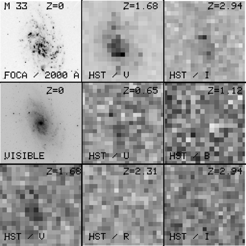
Figure 1: From top to bottom and left to right, this montage presents sequentially the ultraviolet image of M33 at z=0, the redshifted images in V and I uniformely boosted by 4 mag (scenario 3), the visible image of M33 (from the DSS) and the redshifted (scenario 2) images in the UBVRI filters of the WFPC2 (see text and Tab. 2.). Note that these images are not convolved with the HST PSF.

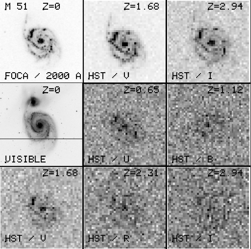
Figure 2: Idem for M51.

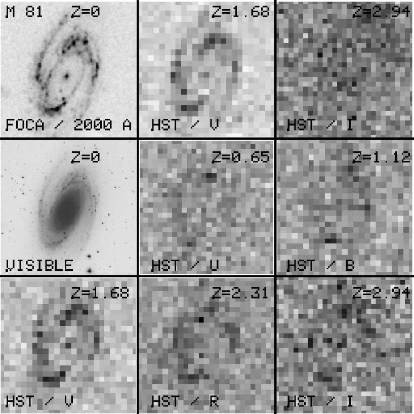
Figure 3: Idem for M81.

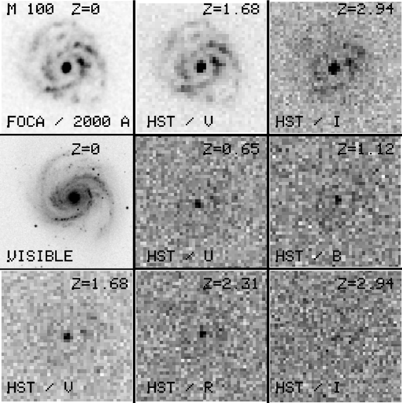
Figure 4: Idem for M100.

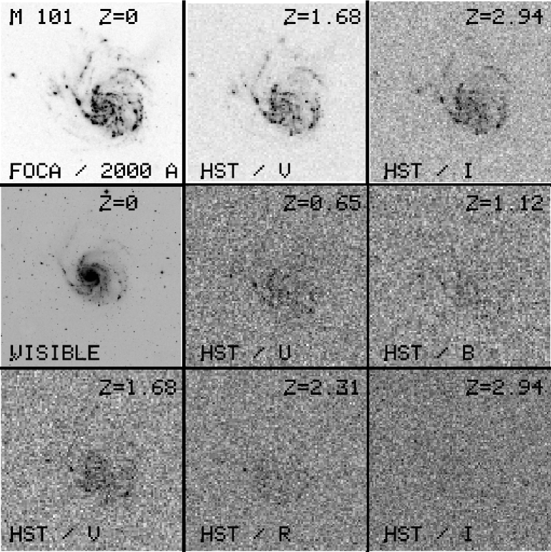
Figure 5: Idem for M101.

3.2 The adopted evolutionary scenarios

Three scenarios have been adopted to move the galaxies away and simulate younger galaxies. First, we simply redshifted them without any modification : no evolution (scenario 1). As we will see below this scenario leads to almost no detections, even at moderate redshifts. Therefore, we assumed some evolution (scenario 2): we adopted an exponential decrease of the star formation rate with an e-folding rate of 8 Gyrs except for M81 which has a e-folding rate of 3 Gyrs. These values are consistent with those expected from the morphological types of the galaxies (e.g. Kennicutt et al. Kennicutt94 (1994)). The adopted evolutionary scenarios translate into a higher UV magnitude when we simulate younger galaxies. The increases in magnitude due to evolution vary with the redshift by 2.5, 3.2, 3.6, 3.9 and 4 mag in U, B, V, R and I respectively for M81 and by 0.9, 1.2, 1.4, 1.5, 1.5 mag in U, B, V, R and I respectively for the other galaxies. However, this evolutionary scenario is not very efficient for the detection of galaxies. For the purpose of actually seeing galaxies and estimating the magnitude needed to observe them, we also applied arbitrary luminosity increases to each pixel of the galaxies from 1 to 4 mag to all the galaxies (see Sect. 5). This last scenario (scenario 3) was only applied to the V-band and I-band or equivalently to the galaxies redshifted to z=1.68 and z=2.94.

4 Detailed properties of the galactic disks

4.1 The surface brightness

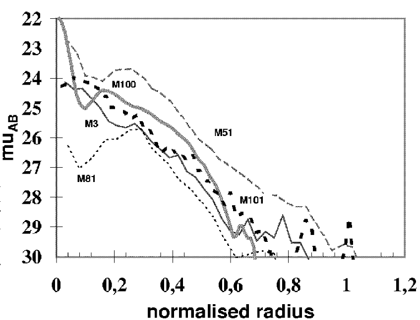
Figure 6: The surface brightness profiles of our galaxy sample observed in UV at z $\approx$ 0. Note that the radii are normalized (see text)

We measured the surface brightness distribution of each galaxy in UV (at z $\approx$ 0) and at different redshifts. The UV rest-frame surface brightnesses are presented in Fig. 6. For comparison, we normalized them to the semi-major axis of the total aperture used for the photometry and defined in section 4.2.1. Whereas M33 and M101 exhibit a rather linear profile, as expected for exponential disks, M51 and M81 have a non-monotonic distribution and M100 may be viewed as an intermediate case. Such a difference in radial profiles will lead to variations in the morphological classification as discussed below. No clear bulge is present in the profiles. Since no recent star formation appears in the bulge, it disappears in UV. These typical morphological changes have been already described in Kuchinski et al. (Kuchinski00 (2000)). M51 is classified as a Seyfert 2 galaxy and M81 as an AGN galaxy but the contribution from the nucleus to the overall UV emission is not important. On the other hand, there is some UV light in the core of M100 which seems to be produced within a nuclear star-formation region (e.g Ryder & Knappen Ryder99 (1999)).

We also calculated the UV surface brightness within the ellipse which encloses half the total light. The measured values are in very good agreement with the predicted values (e.g. Lilly et al.’s Lilly98 (1998)) :

$$\rm\mu_{AB}(z)=\mu_{AB}(RF)+2.5\log(1+z)^{3}-BST$$

$\rm\mu_{AB}(z)$ is the surface brightness observed in the HST filters, $\rm\mu_{AB}(RF)$ the rest frame surface brightness measured in the UV image and BST the boost in magnitude which varies according to the adopted scenario. In this formula we only account for the cosmological dimming term without $\sl K$-corrections since the redshifts were chosen to match the HST filters and to avoid these $\sl K$-corrections.

4.2 Morphological parameters

4.2.1 The half-light radius

The half-light radius ($r_{hl}$) is a basic parameter which measures the size of a galaxy. The critical point is to define the total aperture of the galaxies. We adopt the method detailed in Bershady et al. (Bershady00 (2000)) which defines the total aperture to perform photometry as twice the semi-major axis (called hereafter the major radius) where $\rm\eta(r)=I(r)/<I(r)>=0.2$. Note that $I(r)$ is the local surface brightness and $\rm<I(r)>$ the average surface brightness within the major radius $r$. With such a definition we avoid the need to define isophotal radii which are redshift dependent. In practice, the total flux thus estimated is similar to that deduced from the analysis of the curve of growth. The total UV magnitude of the galaxies at z $\approx$ 0 are reported in Tab. 1.

The half-light major radius was measured in each detected galaxy and the results are reported in Tabs. 3-7. Predicted values were calculated with the measurement at z$\approx$0 and are also reported in these Tables. A remarquable agreement is found between the measured and predicted quantities. In physical units this corresponds to 6 kpc for M81 and M51, 6.8 kpc for M100, 13 kpc for M101 and 3.8 kpc for M33. M101 appears to be very extended: its half-light radius is approximately twice that of M51. As a comparison the ratio of their diameter at B=25 mag ($D_{25}$) is only 1.45. In UV M101 is 0.8 mag brighter than M51 while the difference is of 0.5 mag in B (Tab. 1). M101 is a diffuse object whereas M51 has a very high surface brightness. As expected the detection of M51 at high z is far easier than that of M101 in spite of their absolute luminosity. M81 and M33 are intrinsically fainter with $M_{UV}$ $>$ -18.5 but here again their half-light radii are very different due to their very different UV distribution.

Our conclusion is that the half-light radius appears as a very robust parameter when the galaxy is moved away at high z but only gives a rough estimate of the galaxy size without any morphological information.

4.2.2 The concentration

Kent’s parameter

The concentration parameter is a classical quantity first introduced by Kent (Kent85 (1985)). It is generally defined as the logarithm of the ratio of two radii :

$$\rm C_{K}=5\log(r_{0.8}/r_{0.2})$$

where $r_{0.8}$ is the outer radius enclosing 80$\%$ of the total flux and $r_{0.2}$ is the inner radius enclosing 20$\%$ of the total flux. Such a definition is not based on isophotes and is therefore not dependent on surface brightness dimming as soon as the total aperture to perform photometry is defined independently of isophotal levels. Bershady et al. (Bershady00 (2000)) have found that this parameter is remarkably stable against resolution degradation and conclude that it is very suitable for high redshift measurements.

We calculated the concentration parameter for all the galaxies detected. The aperture to determine the total flux was defined as in the previous section. As expected it appears very stable when the galaxies are redshifted, varying by less than 0.1 as soon as the signal-to-noise ratio (defined within the half-light radius) is larger than 20. However, the absolute values of $C_{K}$ are out of the range usually found for disk galaxies. All the objects exhibit a very low value of $C_{K}$ from 1.5 to 2.6 with $C_{K}(M51)=2$, $C_{K}(M81)=1.5$, $C_{K}(M101)=2.6$, $C_{K}(M100)=2.3$ and $C_{K}(M33)=2.5$ whereas typical values for galactic disks are larger than 3, even for late-type disk galaxies (Kent Kent85 (1985), Bershady et al. Bershady00 (2000)).

This result must be related to the surface brightness profiles presented in Fig. 6. The value of $C_{K}$ for an exponential disk is 2.7, in agreement with the values found for M33 and M101 whose distributions look like exponentials. The very low values found for M51 and M81 are due to their irregular UV distribution with a low central emission and a bright annulus . As already underlined, no bulge is visible. For the five galaxies $C_{K}$ is found too low, due to the absence of a bulge in UV. This result lowers the importance of this parameter for high redshift galaxies observed in a UV rest frame unless a reliable calibration on a large database of templates of all types of galaxies is performed. The calibration made with the Frei sample in B and R are not representative of the UV morphology.

Abraham et al.’s parameter

More recently, Abraham et al. (1996a and references therein) have introduced another definition of the concentration as the ratio of fluxes within two isophotal radii. The outer galaxy isophote is fixed at a given level above the sky (1.5 or 2 $\sigma$) and the inner isophote is defined as having a radius equal to 0.3 times the radius of the outer isophote. The concentration parameter is the ratio of the fluxes between these inner and outer isophotes. Here we adopt the definition:

$$C_{A}={\sum_{E_{\alpha}}I_{ij}\over{\sum_{E_{iso}}I_{ij}}}$$

where $\rm E_{iso}$ refers to the elliptical aperture with a semi major axis ($sma_{iso}$) corresponding to the outer isophote at 1.5 or 2 $\sigma$ and $E_{\alpha}$ to the elliptical aperture with the semi major axis equal to $0.3\cdot sma_{iso}$ (see Fig. 6).

This parameter depends on isophotes and is therefore subject to potential problems since the surface brightness is a steep function of the redshift. This difficulty has lead Bershady et al. to prefer the concentration defined by Kent. Brinchmann et al. (Brinchmann98 (1998)) chose to use Abraham et al.’s concentration (hereafter $C_{A}$) but with a correction of this effect. They assume a de Vaucouleurs law to perform their correction. Such a distribution is certainly not valid for the UV distribution of star forming galaxies. Here we adopt a more empirical approach by directly measuring the concentration on redshifted images of real nearby galaxies.

$C_{A}$ was measured in UV at z $\approx$ 0 for an isophotal level of 1.5 and reported in Tabs. 3-7. The concentration is calculated only when the isophote at the adopted level is closed. All the values found are lower than 0.4 ($\log(C_{A})\leq-0.4$) which is characteristic of spirals and irregulars (e.g. Abraham et al. 1996a ). M81 appears very extreme: this quiescent early-type spiral has a very low concentration. Moreover, the concentration parameter $C_{A}$ of each galaxy is stable when the galaxy is redshifted. The difference $\Delta C_{A}=|C_{A}(z=0)-C_{A}(z\approx 0)|$ $\leq$ 0.16 for all the spiral galaxies studied here except for one value for M33 (scenario 3 and boost by 4 mag) which has a large uncertainty.

Therefore Abraham et al.’s concentration parameter appears as a robust one. It is more adequate than Kent’s one to describe the UV morphologies at low and high redshifts.

Table 3: Detectability and morphology of Messier 51. In the first part of the table, the galaxy is redshifted assuming an exponential evolution with $\tau=$ 8 Gyr, in the second and third parts of the table the galaxy is boosted by a constant factor (1 to 4 mag) and redshifted in the V band (z=1.68) and in the I band (z=2.94). The concentration and asymmetry are defined as by Abraham et al. The concentration is calculated at the 1.5$\sigma$ level. The symbol “:” after a value points out its large uncertainty, $SB$ means surface brightness within the half-light radius $r_{hl}$ in m_AB/arcsec² and $\Delta$ V and $\Delta$ I the brightening in V and I. The symbol “nd” means that the galaxy was not detected in this filter

Filter	UV	U	B	V	R	I
z	0	0.65	1.12	1.68	2.31	2.94
S/N	$5000$	18	13	26	15	9
$\rm m_{AB}$	11.2	23.5	24.0	24.9	25.1	25.3
$\rm r_{hl}(")$	151	0.75	0.75	0.70	0.78	0.84
pred. $\rm r_{hl}$		0.77	0.73	0.72	0.77	0.83
$A$	0.26	0.3:	0.4:	0.31	0.35	0.4:
$C_{A}$	0.29	0.17		0.17
SB	23.7	24.5	25	25.7	26.2	26.5
$\Delta$ V	0 mag	1 mag	2 mag	3 mag	4 mag
S/N	8	20	50	130	300
$\rm m_{AB}$	26	25	24	23	22
$\rm r_{hl}(")$	0.61:	0.79	0.73	0.75	0.73
$A$	0.5:	0.27	0.30	0.28	0.26
$C_{A}$		0.17	0.18	0.23	0.25
SB	26.8	26	25	24	23
$\Delta$ I	0 mag	1 mag	2 mag	3 mag	4 mag
S/N	nd	7	12	28	70
$\rm m_{AB}$		25.6	24.9	24	23
$\rm r_{hl}(")$		0.73:	0.8	0.8	0.8
$A$		0.6:	0.35	0.28	0.25
$C_{A}$				0.17	0.17
SB		26.5	26	25.2	24.2

Table 4: Detectability and morphology of Messier 81. Same as table 3 but with $\tau$ = 3 Gyrs

Filter	UV	U	B	V	R	I
z	0	0.65	1.12	1.68	2.31	2.94
S/N	$3000$	10	10	30	20	10
$\rm m_{AB}$	11.7	24.3	24.3	24.5	24.6	25.2
$\rm r_{hl}(")$	366	0.76	0.72	0.79	0.87	0.8
pred. $\rm r_{hl}$		0.79	0.72	0.74	0.78	0.84
$A$	0.21	0.4:	0.5:	0.32	0.36	0.3:
$C_{A}$	0.09			0.08	0.05
SB	26	25.3	25.2	25.6	25.8	26.3
$\Delta$ V	0 mag	1 mag	2 mag	3 mag	4 mag
S/N	nd	nd	8	20	45
$\rm m_{AB}$			26.5:	25.3	24.4
$\rm r_{hl}(")$			0.7:	0.75	0.73
$A$			0.4:	0.38	0.25
$C_{A}$				0.06	0.09
SB			27	26.2	25.2
$\Delta$ I	0 mag	1 mag	2 mag	3 mag	4 mag
S/N	nd	nd	nd	nd	8
$\rm m_{AB}$					25.3
$\rm r_{hl}(")$					0.8
$A$					0.3:
$C_{A}$
SB					26.4

Table 5: Detectability and morphology of Messier 101. Same as table 3.

Filter	UV	U	B	V	R	I
z	0	0.65	1.12	1.68	2.31	2.94
S/N	$5000$	20	14	26	15	nd
$\rm m_{AB}$	10	22.5:	23.4:	24	24.4:
$\rm r_{hl}(")$	384	1.63:	1.4:	1.56	1.4:
pred. $\rm r_{hl}$		1.66	1.52	1.54	1.65	1.78
$A$	0.40	0.39	0.5:	0.41
$C_{A}$	0.30			0.19
SB	24.5	25.4	25.9	26.5	27
$\Delta$ V	0 mag	1 mag	2 mag	3 mag	4 mag
S/N	10	20	47	115	290
$\rm m_{AB}$	25.7:	24.3	23.3	22.2	21.1
$\rm r_{hl}(")$	1.1:	1.3:	1.5	1.45	1.5
$A$		0.6:	0.33	0.40	0.40
$C_{A}$		0.17	0.14	0.25	0.30
SB	27.8:	26.8	25.9	24.9	23.9
$\Delta$ I	0 mag	1 mag	2 mag	3 mag	4 mag
S/N	nd	nd	10	25	64
$\rm m_{AB}$			24.1	23.1	22
$\rm r_{hl}(")$			1.7:	1.86	1.9
$A$			0.5:	0.42	0.39
$C_{A}$					0.14
SB			27.3	26.3	25.3

Table 6: Detectability and morphology of Messier 33. Same as table 3.

Filter	UV	U	B	V	R	I
z	0	0.65	1.12	1.68	2.31	2.94
S/N	$5500$	3	nd	6	nd	nd
$\rm m_{AB}$	9.0	26.2		26.9
$\rm r_{hl}(")$	889	0.4:		0.4:
pred. $\rm r_{hl}$		0.49	0.44	0.45	0.48	0.52
$A$	0.31			0.6:
$C_{A}$	0.33
SB s	25	26		26.7
$\Delta$ V	0 mag	1 mag	2 mag	3 mag	4 mag
S/N	nd	4	10	26	60
$\rm m_{AB}$		27.4	26.5	25.5	24.5
$\rm r_{hl}(")$		0.3:	0.4:	0.38	0.40
$A$			0.5:	0.5:	0.5:
$C_{A}$				0.23	0.24
SB		26.7	25.9	24.9	23.9
$\Delta$ I	0 mag	1 mag	2 mag	3 mag	4 mag
S/N	nd	nd	nd	5	13
$\rm m_{AB}$				26.6	25.5
$\rm r_{hl}(")$				0.44	0.55
$A$				0.6:	0.4:
$C_{A}$					0.06:
SB				26.3	25.5

4.2.3 The asymmetry

Asymmetry is one of the most natural way of analyzing morphology and classifying galaxies. Conselice et al. (Conselice00 (2000)) present a detailed study of rotational asymmetry in galaxies. Here, we define the asymmetry in the same way as Abraham et al. (1996a ) :

$$A=1/2(min[{\Sigma|I_{0}-I_{\Phi}|\over\Sigma|I_{0}|}]-min[{\Sigma|B_{0}-B_{\Phi}|\over\Sigma|I_{0}|}])$$

where $I$ represents the image pixel values and $B$ the background pixel values. The rotation angle $\Phi$ is set to 180 $\deg$ in this paper, which means that the I_Φ images are rotated by 180 $\deg$ before subtraction with the original image. The first term on the right side of the equation corresponds to the asymmetry of the source. Note, however, that the rotational asymmetry is a measurement based on individual pixels and noise poses an important problem. Consequently, Conselice et al. (Conselice00 (2000)) introduce a noise correction (only valid for uncorrelated noise and therefore not for HDF dithered images) which is computed in the latter term. This correction consists of estimating the asymmetry of blank areas in the neighborhood of the galaxy. In order to optimize this calculus we must check that the computed asymmetry is really at a minimum and an additional step is to compute $A$ at different positions on a grid and keep the minimum value. Another key-point lies in the signal-to-noise ratio. In this paper, we computed $A$ for all detected galaxies. In agreement with Conselice et al. (Conselice00 (2000)), we computed the asymmetry up to the radius where $\eta$ = 0.2 ($\eta(r)$ = ${I(r)\over<I(r)>}$), which permits us to define a maximum radius independent of the distance/redshift and of the photometric calibration. The half-light integrated S/N must exceed $\sim$ 20 in order to have reliable estimates for A. This is less than the limiting S/N values reached by Conselice et al. (Conselice00 (2000)). As expected, the galaxies appear very asymmetric with $A>0.2$. This point will be discussed in Sect. 6.

Table 7: Detectability and morphology of Messier 100. Same as table 3.

Filter	UV	U	B	V	R	I
z	0	0.65	1.12	1.68	2.31	2.94
S/N	1600	14	10	20	11	nd
$\rm m_{AB}$	12.6	23.6	24.2	24.6	25.2
$\rm r_{hl}(")$	88	0.82	0.82	0.88	0.8:
pred. $\rm r_{hl}$		0.90	0.79	0.81	0.86	0.93
$A$	0.20	0.45	0.5:	0.37	0.45
$C_{A}$	0.25
SB	24.4	25.1	25.6	26.3	26.7
$\Delta$ V	0 mag	1 mag	2 mag	3 mag	4 mag
S/N	nd	15	35	83	210
$\rm m_{AB}$		27.4	26.5	25.5	24.5
$\rm r_{hl}(")$		0.9:	0.82	0.82	0.84
$A$		0.4:	0.24	0.22	0.22
$C_{A}$			0.21	0.21	0.22
SB		26.8:	25.7	24.7	23.7
$\Delta$ I	0 mag	1 mag	2 mag	3 mag	4 mag
S/N	nd	nd	7	20	50
$\rm m_{AB}$			25.2:	24.1	23.1
$\rm r_{hl}(")$			0.9	0.98	1.0
$A$				0.30	0.20
$C_{A}$					0.21
SB			26.9	25.9	25

5 Detection of disks at high redshifts

The first question that we will address is the detectability of disks at high redshifts. The evolution of the B mean surface brightness of large disk-dominated galaxies was thought to increase by a value of $\Delta\mu$ ranging from 0.8 to 1.6 mag between now and a redshift of z $\approx$ 1 compared to Freeman’s (Freeman70 (1970)) value at z = 0 (Schade et al. Schade96 (1996); Lilly et al. Lilly98 (1998); Roche et al. Roche98 (1998), Bouwens & Silk Bouwens00 (2000)). However, Simard et al. (Simard99 (1999)) performed a similar analysis but took into account a selection function in the magnitude-size plane as a function of redshift. The main effect produced by the above bias is that galaxies with low surface brightnesses are lost at high redshit. Before correction, the mean disk surface brightness would increase by $\Delta\mu$ = 1.3 mag from z=0.1 to z=0.9 consistently with the values estimated by Schade et al. (Schade96 (1996)), Lilly et al. (Lilly98 (1998)), Roche et al. (Roche98 (1998)). After accounting for the selection effect, no discernible evolution is observed in the disk surface brightness of disk-dominated galaxies brighter than $M_{B}$ = -19. However, using the same dataset Bouwens & Silk (Bouwens00 (2000)) reach a different conclusion ($\Delta\mu$ $\sim$1.5 mag of evolution). This difference stems from the fact that Bouwens & Silk (Bouwens00 (2000)) find, in the observation, a number of high surface brightness galaxies exceeding model predictions. These authors therefore argue that there is a strong evolution in the total number of high surface brightness galaxies from z = 0 to z $\approx$ 1 not accounted for by Simard et al. (Simard99 (1999)).

We can analyze the detectability of our simulated high-redshift observations in HST bands. The first point to note is that M33, M81 and M100 become undetectable if they are redshifted in the HST V-band (z=1.68) without any other modifications. The situation is only more favourable for M51 and M101 which are detected in the V-band with an integrated S/N $\approx$ 10. Note that the S/N are measured within ellipses which enclose half the total light of the galaxy. Even when detected, these low S/N prevent any safe estimations of morphological parameters as discussed below. None of the galaxies are detected in the HST I-band (z=2.94). The results for the V-band and I-band without evolution are reported in Tabs. 3-7 (referred to as a brightening of 0 mag). The V-band appears as the best configuration to maximize S/N as it combines a rather moderate redshift (z=1.68) with an efficient filter (f555W).

In the following we will use scenario 2 of luminosity evolution presented in Sect. 3.2 for the galaxies and analyze their effect on the detectability of the spiral galaxies. For all the galaxies other than M81, this scenario implies an evolution of the surface brightness consistent with the values found in the literature and presented at the beginning of the section. The S/N barely reaches 30, i.e. below the value of 50 which is considered by Conselice et al. (Conselice00 (2000)) as necessary to begin to estimate reliable morphological parameters. It seems, however that some reasonably safe work can be carried out down to S/N $\approx$ 20-30, depending on the galaxies (see Sect. 5.2). The adopted evolutionary scenario is not enough for M33 and S/N $<$ 10. For the other spiral galaxies, 10 $\leq$ S/N $\leq$ 30. Nevertheless, in only a limited number of cases, $A$ and $C_{A}$ can be safely estimated. If such galaxies are observed at high redshift, it would be often impossible to perform a reliable morphological analysis.

In order to constraint the evolution needed to detect our local spiral galaxies and estimate their morphological parameters, we applied scenario 3, i.e. a uniform magnification (same one to each pixel of the image) ranging from 1 to 4 magnitudes to our galaxies observed at z=1.68 and z=2.94 i.e. observations through the WFPC2 V-f555W and I-f814W filters. In the V-band, S/N $\geq$ 20 is the minimum needed to perform any morphological analysis. M51 reaches such a value with a boost of 1 mag. This boost is slightly less that the V-boost adopted in scenario 2 and explains the positive results for this filter. Assuming H₀=50 km.s^-1.Mpc^-1 and q₀=0.5, this translates into an e-folding rate slightly larger than in scenario 2 : $\tau_{V}=10.9$ Gyrs.

The high surface brightness of M51 is the major characteristic that helps detection of this spiral galaxy. A boost by 2 mag (i.e. $\tau_{V}=5.5$ Gyrs) is needed for M100 and M101 to get reliable morphological parameters. Up to 3 mag (i.e. $\tau_{V}=3.6$ Gyrs) and more than 4 mag (i.e. $\tau_{V}=2.7$ Gyrs) are necessary to measure $A$ and $C_{A}$ in V. The situation is slightly worse in the I-band where a reliable estimate of the morphology corresponds to a boost by 3 mag ($\tau_{I}=4.1$ Gyrs) for M51, by 4 mag ($\tau_{I}=3.1$ Gyrs) for M100 and M101 with the same assumptions on the cosmology. M33 and M81 are never detected in I, which implies boost $>$ 4 mag (i.e. $\tau_{I}\leavevmode\nobreak\ >\leavevmode\nobreak\ 3$ Gyrs) for a detection. Such evolutions are very high and imply e-folding rates more typical of very early type galaxies dominated or largely influenced by the bulge component. Roche et al. (Roche98 (1998)) found $\sim$ 2.8 mag of surface brightness evolution for galaxies at 2 $<$ z $<$ 3.5 relative to galaxies at z $<$ 0.35.

In conclusion, except perhaps for spiral galaxies with the high surface brightnesses (evolution $>$ 3 mag) which may be detected at high redshift with a good S/N, it would not be possible to get reliable estimates of their morphological parameters $A$ and $C_{A}$ and therefore to classify them at z$>$2. In Fig. 7 we compare the detection limit (with an exposure time of 2.5 ksec) reached by Roche et al. (Roche96 (1996)) in the ($Log(r_{hl})$ vs. $I_{AB}$) diagram for I-band exposures to our measured values (in the I-band as well). It was necessary to change Roche et al.’s (Roche96 (1996)) Johnson I magnitudes to the AB systems by applying the relation $I_{AB}=I+0.52$. Our spiral galaxies could have been detected by Roche et al. (Roche96 (1996)) assuming boosts $\geq$ 1-2 mag for M51, M100 and M101 but boosts $\geq$ 3-4 mag for M33 and M81. The size of M101 is in the upper bin in the $r_{hl}$ distribution presented by Roche et al. (Roche98 (1998)). The other galaxies have $r_{hl}$ in the observed range.

Note that our simulations are more optimistic that actual HST observations (see Sect. 3), and it would be even more difficult to detect them. However, the detection is not the whole story and an additional caveat appears. We have only been able to quantitatively estimate the asymmetries and concentration for M51, M100 and M101 with large boosts. This means that we would not be able to classify those galaxies unless very large boosts were applied to the brightest galaxies. Moreover, as we will see in the next section, these galaxies would not appear as spirals anyway.

Models of galaxy formation in hierarchical cold dark matter (CDM) cosmogonies predict that Milky Way-like disks cannot form at $z>1$ in a universe with $\Omega_{0}\sim 1$ while lower constraints come from a low-$\Omega_{0}$ universe (Mo et al. Mo98 (1998)). Note, however, that these scenarios predict that early disks may be present at high redshifts but with a size significantly smaller than the disks observed today. From an analysis of the NTT Deep Field, Poli et al. (Poli99 (1999)) found that the size distribution of a sample of disk-dominated galaxies peaks at very small sizes, $r_{hl}\approx 2.5$ kpc, corresponding in their sample to $r_{hl}\approx$ 0.3 $arcsec$. This is also consistent with the HST Medium Deep Survey (MDS) results (Roche et al. Roche98 (1998)). Comparing their results to the CDM predictions, Poli et al. (Poli99 (1999)) show a general agreement but noticed a possible excess of faint, small-sized galaxies. Our simulations show that we could not draw any definite conclusions on the existence of large spiral disks at redshifts $z>1$ as stated by Mao, Mo and White (Mao98 (1998)). Actually, the observational constraints from the fact that we could not detect them with the HST and NTT are too small.

What are the disk-dominated galaxies seen by Roche et al. (Roche98 (1998)) at z $\approx$ 3-4 and Poli et al. (Poli99 (1999)) at I $\leq$ 25 ? Our simulations show that we do not expect any variations of the size with the redshift due to dimming of surface brightness. Roche et al. (Roche98 (1998)) conclude that the $r_{hl}$ distributions are in agreement with a size-luminosity evolution model where spiral galaxies undergo a small size evolution below z $\leq$ 1.5 but are smaller by a factor of the order of 2 at z $\approx$ 3. In addition, Mo et al. (Mo98 (1998)) models for the formation of galactic disks would tend in the same direction. It is therefore a subject that deserves further work and we will analyze, in a follow-up paper, scenarios where we vary the size of the disk assuming, for instance, a radial variation of the star formation history as in Roche et al. (Roche96 (1996)).

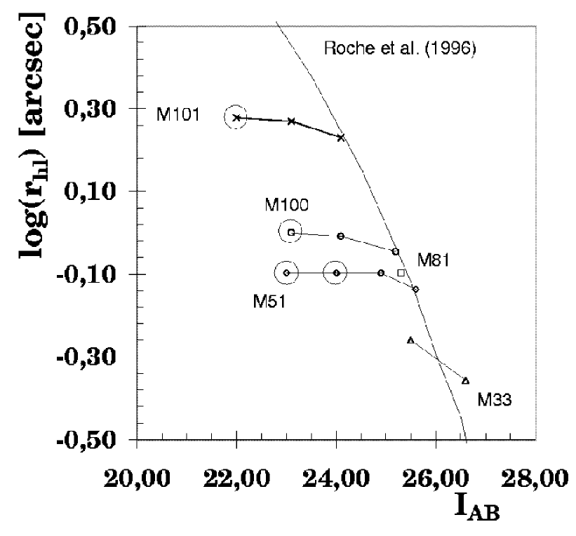
Figure 7: The location of the galaxies when detected in the I-band in the log of the half-light radius log($r_{hl}$) in arcsecs vs. the $I_{AB}$ magnitude within $r_{hl}$. The line corresponds to the detection limit modelled by Roche et al. (Roche96 (1996)) and scaled to $I_{AB}$. It can be seen than M33 and M81 are only marginally detectable within our modelled evolution. M51, M100 and M101 can be detected with lower boosts but their morphology cannot be measured except for the major boosts which are shown with large circles around the symbols.

6 Morphology of disks at high redshifts

Using our own sample of local spiral galaxies observed in UV with FOCA, we simulate high-redshift observations and we also estimate asymetries and concentration for our simulated galaxies. Tabs. 3-7 and Fig. 8 present our results. Fig. 8 is the (Log $A$ vs. log $C_{A}$) diagram where the dotted lines represent the separations of Hubble types reported by Abraham et al. (1996b ). As noted above, we have assumed several scenarios for the luminosity evolution. The first point to note is that all the galaxies fall in the top-left area corresponding to the irr/pec/mrg galaxies. We do confirm the previous qualitative results that spiral galaxies observed in a UV rest-frame appear more irregular. Indeed, this effect is clearly present even at z $\approx$ 0 but it must be pointed out the the morphology is very stable and does not change with the redshift. From z=0 to the highest explored redshifts, we observed similar concentrations and asymmetries for a given galaxy. The migration of spiral galaxies towards more asymetrical areas is mainly caused by the clumpiness of the star formation regions observed in UV. The symbols corresponding to the redshifted galaxies in the HST filters fall very close to their z $\approx$ 0 parent galaxy. Galaxies where the evolution is assumed to be proportional to e^-t/τ fall in the diagram at -1.4 $\leq$log $C_{A}$ $\leq$ -0.5. This quite large range is in fact due to M81 (log $C_{A}\leq$ -1.0) whereas the other galaxies show similar concentrations (-0.9 $\leq$log $C_{A}$ $\leq$ -0.5). Moreover, note that the concentration is not consistent with the usual values measured in the visible. Indeed, M81 is the most early-type galaxy but appears as the least concentrated galaxy in Fig. 8. Clearly, more UV templates must be studied to test concentration as a morphological discriminator between early and late type galaxies. All spiral galaxies lie in a very narrow log A range (-0.7 $\leq$ log A $\leq$ -0.2). They are very asymmetric compared to their optical morphology and are located in the irregular domain. Furthermore, the degeneracy of the log $A$ parameter in UV is very limiting for morphology studies. Other ways of measuring the asymmetry have been studied. For instance, Rudnick & Rix (Rudnick98 (1998)) use the Fourier amplitudes of the image. Kornreich et al. (Kornreich98 (1998)) compare the relative fluxes of trapezoidal areas distributed around the center of the galaxy. Even for scenarios where the galaxy is uniformely boosted by a magnitude ranging from 0 $\leq$ $\Delta m$ $\leq$ 4, the increase of S/N does not change our conclusion and the galaxies remain in the same area whatever the scenario. This large asymmetry - low concentration morphology is intrinsic to the UV.

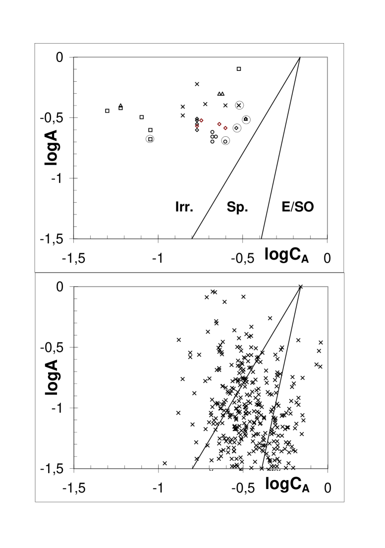
Figure 8: Upper panel : the distribution of our sample of rest-frame and artificially redshifted galaxies in the log $A$ versus log $C_{A}$ asymmetry-concentration diagram. The redshifted galaxies are all lying in the irregular area as defined at visible wavelengths by Abraham et al. (1996b ). An important result, however, is that rest-frame ultraviolet spiral galaxies are found in this area as well. This confirms the important role of the observation wavelength range. On this basis, we should therefore expect no or little morphology evolution of the spiral galaxies with the redshift. The lower panel shows as a comparison the classification of galaxies in the HHDF (Abraham et al. 1996b ). The symbols are defined as follows : triangle for M33, diamond for M51, box for M81, circle for M100 and cross for M101. Symbols within a larger circle represent galaxies at z $\approx$ 0.

7 Conclusion

The main results of this paper are summarized as follows :

• As expected, galaxies observed in UV are very different from their visible counterpart as the young populations are predominent. These galaxies appear more clumpy.

• Local galaxies with large disk projected at high redshift (0.65 $\leq$ z $\leq$ 2.94) would be hardly detected with the HST in 10-hr exposure times. Consequently, no strong observational constraints can be set on the presence or absence of large galaxy disks at high z.

• A quantitative analysis of the UV morphology of disk galaxies shows that there is a clear trend for spirals to move towards more irregular morphology types (morphological K-correction). If the concentration parameter appears to be a good discriminator between early and late type galaxies, the asymmetry is degenerate and all the galaxies have very similar asymmetry values. New ways of measuring the asymmetry need to be explored.

• The location of a given galaxy in the (log $A$ vs. log $C_{A}$) diagram is very stable and does not depend on the redshift or the S/N as soon as the rest-frame wavelength is in UV. Therefore, rest-frame visible imaging is not helpful and it would be useful to define a multi-wavelength morphology system.

This paper stresses the need to keep on working on the UV morphology of galaxies if we wish to be able to understand the objects observed at high redshift. It is therefore necessary to define new tools for classifying galaxies. A number of objects have been observed by FOCA, UIT-Astro-2 and other UV imagers. However, the database is still too small for a significative study. Hopefully, GALEX, the GALaxy Evolution eXplorer will complete a UV survey of the sky within the next years and the accumulated data will be crucial to progress in the understanding of the formation and evolution of galaxies.

- (1) Abraham R.G., van den Bergh S., Glazebrook K., Ellis R.S., Santiago B.X., Surma P., Griffiths R.E. 1996b, ApJS 107, 1
- (2) Abraham R.G., Tanvir N.R., Santiago B.X., Ellis R.S., Glazebrook K., van den Bergh S. 1996a, MNRAS 279, L47
- (3) Bershady M.A., Jangren A., Conselice C.J. 2000, AJ (June 2000, in press)
- (4) Bohlin R.C., Cornett R.H., Hill J.K., Robert S., Landsman W.B., O’Connell R.W., Neff S.G., Smith A.M., Stecher T.P. 1991, ApJ 368,12
- (5) Bouwens R.J., Silk J. 2000, astro-ph/0002133
- (6) Brinchamnn J., Abraham R., Schade D., Tresse L., Ellis R.E., Lilly S., Le Fèvre O., Glazebrook K., Hammer F., Colless M., Crampton D., Broadhurst T. 1998, ApJ 499, 112
- (7) Bunker A., Spinrad H., Stern D., Thompson R., Moustakas L., Davis M., Dey A. 2000, astro-ph/0004348
- (8) Conselice C.J., Bershady M.A., Jangren A. 2000, ApJ 529, 886
- (9) Driver S.P., Fernandez-Soto A., Couch W.J., Odewahn S.C., Windhorst R.A., Phillips S., Lanzetta K., Yahil A. 1998, ApJ 496, 93
- (10) Feldmeier J.J., Ciardullo R., Jacoby G.H. 1997, ApJ 479, 231
- (11) Ferrarese L., Freedman W.L., Hill R.J. et al. 1996, ApJ 464, 568
- (12) Freeman K. 1970, ApJ 160, 811
- (13) Frei Z., Guhathakurta P., Gunn J.E., Tyson J.A. 1996, AJ 111, 174
- (14) Giavalisco M., Livio M., Bohlin R.C., Macchetto F.D., Stecher T.P. 1996a, AJ 112, 369
- (15) Giavalisco M., Steidel C.C., Macchetto F.D. 1996b, ApJ 470,189
- (16) Holtzman J., Hester J.J., Casertano S. et al. 1995, PASP 107, 156
- (17) Kornreich D.A., Haynes M.P., Lovelace R.V.E. 1998, AJ 116, 2154
- (18) Huterer D., Sasselov D.D.. Schechter P.L. 1995, AJ 110, 2705
- (19) Kennicutt R.C., Tamblyn P., Congdon C.E. 1994, ApJ 435, 22
- (20) Kent S.M. 1985, ApJS 59, 115
- (21) Kuchinski L.E., Freedman W.L., Madore B.F., Trewhella M., Bohlin R.C., Cornett R.H., Fanelli M.N., Marcum P.M., Neff S.G., O’Connell R.W., Roberts M.S., Smith A.M., Stecher T.P., Waller W.H., 2000, astro-ph/0002111 (ApJS in press)
- (22) Lilly S., Schade D., Ellis R. et al. 1998, ApJ 500, 75
- (23) Lowenthal J.D., Koo D.C., Guzman R., Gallego J., Phillips A.C., Faber S.M., Vogt N.P., Illingworth G.D., Gronwall G. 1997, ApJ 481, 673
- (24) Mao S., Mo H.J. and White S.D.M. 1998, MNRAS 297, L71
- (25) Milliard B., Donas J., Laget M., Armand C., Vuillemin A. 1992, A&A 257,24
- (26) Mo H.J., Mao S., White S.D.M. 1998, MNRAS 295, 319
- (27) Poli F., Giallongo E., Menci N., D’Odorico S., Fontana A. 1999, ApJ 527, 662
- (28) Roche N., Ratnatunga K., Griffiths R.E., Im M., Naim A. 1998, MNRAS 293, 157
- (29) Roche N., Ratnatunga K., Griffiths R.E., Im M., Neuschaefer L. 1996, MNRAS 282, 1247
- (30) Rudnick G., Rix H.W. 1998, AJ 116, 1163
- (31) Ryder S.D., Knapen J.H. 1999, MNRAS 302, 7
- (32) Schade D., Lilly S.J., Le Fèvre O., Hammer F., Crampton D. 1996, ApJ 464, 79
- (33) Shara M.,M., Sandage A., Zurek D.R. 1999, PASP 111, 1367
- (34) Simard L., Koo D.C., Faber S.M., Sarajedini V.L., Vogt N.P., Phillips A.C., Gebhardt K., Illingworth G.D., Wu K.L. 1999, ApJ 519, 563
- (35) Steidel C.C., Giavalisco M., Dickinson M., Adelberger K.L. 1996, AJ 112, 352
- (36) Stetson P.B., Saha A., Ferrarese L. et al. 1998, ApJ 508, 491
- (37) Tully R.B., Richard F.J. 1988 in Catalog of Nearby Galaxies, ISBN 0521352991, Cambridge University Press
- (38) van den Bergh S., Abraham R.G., Ellis R.S. Tanvir N.R., Santiago B.X., Glazebrook K.G. 1996, AJ 112, 359