Chapter 1 Evolution of galaxies due to self-excitation

Martin D. Weinberg
Department of Physics & Astronomy, University of Massachusetts, Amherst, MA 01003-4525, USA

1 Introduction

These lectures will cover methods for studying the evolution of galaxies since their formation. Because the properties of a galaxy depend on its history, an understanding of galaxy evolution requires that we understand the dynamical interplay between all components over 10 gigayears. For example, lopsided ($m=1$) asymmetries are transient with gigayear time scales, bars may grow slowly or suddenly and, under circumstances may decay as well. Recent work shows that stellar populations depend on asymmetry.

The first part will emphasize n-body simulation methods which minimize sampling noise. These techniques are based on harmonic expansions and scale linearly with the number of bodies, similar to Fourier transform solutions used in cosmological simulations. Although fast, until recently they were only efficiently used for small number of geometries and background profiles. I will describe how this so-called expansion or self-consistent field method can be generalized to treat a wide range of galactic systems with one or more components. We will work through a simple but interesting two-dimensional example relevant for studying bending modes.

These same techniques may be used to study the modes and response of a galaxy to an arbitrary perturbation. In particular, I will describe the modal spectra of stellar systems and role of damped modes which are generic to stellar systems in interactions and appear to play a significant role in determining the common structures that we see. The general development leads indirectly to guidelines for the number of particles necessary to adequately represent the gravitational field such that the modal spectrum is resolvable. I will then apply these same excitation to understanding the importance of noise to galaxy evolution.

2 N-body simulation using the expansion method

2.1 Potential solver overview

A number of n-body potential solvers have already been mentioned in other lectures. To better understand the motivation for the development here, I will begin by briefly reviewing and contrasting their properties. Many of these have already been reviewed by Hugh Couchman but I would like to make a general point to start: the n-body problem of the galactic dynamicist or cosmologist differs considerably from the n-body problem of the celestial mechanician or the student of star clusters. For galactic or CDM simulations, one really wants a solution to the collisionless Boltzmann equation (CBE), not the an n-body system with finite $N$. A direct solution of the CBE is not feasible, so simulate a galaxy by an intrinsically collisional problem of n-bodies but with parameters that best yield a solution to the CBE. In other words, you should consider an n-body simulation in this application as algorithm for Monte Carlo solution of the CBE. The $N$ bodies should be considered tracers of the density field that we simultaneously use to solve for the gravitational potential and sample the phase-space density.

2.1.1 Direct summation: the textbook approach

This truly is the standard n-body problem. The force law is the exact pairwise combination of central force interactions; there are $\left({N\atop 2}\right)={N!\over(N-2)!2!}={N(N-1)\over 2}$ couplings. One might use Sverre Aarseth’s advanced techniques for studying star clusters or various special purpose methods to study the solar system as Tom Quinn and others have reviewed in this volume.

Considered as a solution to the CBE, the density is a distribution of points and the force from pairwise attraction of all points. For any currently practical value of $N$, this system is a poor approximation to the limit $N\rightarrow\infty$. Furthermore, the direct problem is is this very expensive. Of course, this direct approach is easy to understand, implement, and with appropriate choice of softening parameter is useful in some cases. However in most cases, it makes sense to take a different approach: interpret the distribution of $N$ points as a sampling of the true distribution. This motivates tree and mesh codes among others.

2.1.2 Tree code

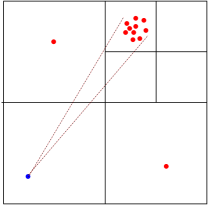
(a) Tree algorithm

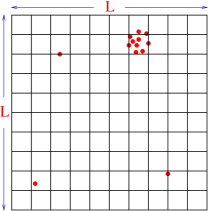
(b) Mesh algorithm

Figure 1: Construction of the data structure for the tree algorithm in two dimensions (a) illustrating the opening angle and (b) the mesh algorithm.

The tree algorithm makes use of differences in scales to only do the computational work that will make a difference to the end result. The algorithm treats distant groups of particles as single particles at their centers of mass. The criterion for replacing a group by a single particle is whether or not the angular subtent of that group is smaller than some critical opening angle $\theta_{c}$. Figure 1 shows the recursive construction that gives the tree code it’s name. This particular tree is a quad tree although k-d trees and others have been used. The force computation only “opens” the nodes of the tree if they are larger than $\theta_{c}$. Thinking in terms of multipole expansions, one is keeping multipoles up to order $l\sim 2\pi/\theta_{c}$; typical opening angles have $l\mathrel{\hbox to0.0pt{\lower 3.0pt\hbox{$\mathchar 536\relax$}\hss}\raise 2.0pt\hbox{$\mathchar 318\relax$}}20$.

2.1.3 Mesh code

A mesh code is simple in concept. The steps in the algorithm are as follows. First, assign the particle distribution to bins. Be aware there are good and bad ways of doing this. For example, one may wish distribute the mass of a particle according to a smoothing kernel rather than using the position and bin boundaries naively. Then, represent density as a Fourier series by performing a discrete Fourier transform by FFT. Again, one must be very careful about boundary conditions; see Couchman’s paper in this volume and references therein. Finally, the gravitational potential follows directly from Fourier analysis: $\rho=\sum_{\bf k}c_{\bf k}e^{i{\bf k}\cdot{\bf x}}$ and by a simple application of the Poisson equation, this yields $\Phi=-\sum_{\bf k}c_{\bf k}\exp({i{\bf k}\cdot{\bf x})}/4\pi Gk^{2}$.

In short, we are using a mesh to represent the density and exploiting harmonic properties of the Poisson equation to write down the gravitational potential. Note that the particle distribution traces the mass but an individual particle does not interact with others as a point mass.

2.1.4 SPH

This notion of density representation is explicit in smoothed-particle hydrodynamics (SPH), a topic which has also appeared several times in these lectures. In SPH, the gas particles must be considered as tracers of the gaseous density, temperature, and velocity fields. The hydrodynamic equations are solved, crudely speaking, by a finite difference solution on an appropriately smoothed fields determined from the tracers. One can show that these algorithms reduce to Euler’s equations in the limit of large $N$. The choice of algorithm and smoothing kernel must be done with great care but most clearly, the gas particles are not stars or gas clumps in any physical sense but tracers of field quantities.

2.1.5 Summary

All of these but direct summation are examples of density estimation: a statistical method for determining the density distribution function based on a sample of points. The algorithms follow the same pattern: (1) Estimate the density profile of the galaxy based on the $n$ bodies; (2) Exploit some property of the estimation to efficiently compute the gravitational potential, and in the case of SPH, other necessary field quantities; (3) Use the gravitational field to derive the accelerations, and in the case of SPH, the hydrodynamical equations of motion.

2.2 Expansion method

The expansion method is density estimation using an orthogonal function expansion. This is a standard technique in functional approximation and familiar to most readers. Its application to solving the Poisson equation is directly analogous to the grid method. In the standard grid method, one represents the density as a Fourier series

$$\rho({\bf r})={1\over L^{3}}\sum_{l,m,n=-M}^{M}c_{lmn}e^{i\Delta k(lx+my+nz)}$$ (1)

where $\Delta k=2\pi/L$ and the infinite sum of integer is truncated at $\pm M$. Then, by separation of variables, the gravitational potential is:

$$\Phi({\bf r})=-{1\over 4\pi G(\Delta k)^{2}}{\sum^{M}_{l,m,n=-M}}^{\prime}c_{lmn}{e^{i\Delta k(lx+my+nz)}\over l^{2}+m^{2}+n^{2}}.$$ (2)

There is a way to skip the binning and FFT steps altogether. We can write the density profile of the $n$ point particles as

$$\rho(x,y,z)=\sum_{i=1}^{N}\delta(x-x_{i})\delta(y-y_{i})\delta(z-z_{i})$$ (3)

The coefficient $c_{lmn}$ is integral

$${1\over L^{3}}\int^{L/2}_{-L/2}dx\int^{L/2}_{-L/2}dy\int^{L/2}_{-L/2}dze^{-i\Delta k(lx+my+nz)}\rho(x,y,z)$$ (4)

which immediately yields

$$c_{lmn}={1\over L^{3}}\sum_{i=1}^{N}e^{-i2\pi lx_{i}/L}e^{-i2\pi my_{i}/L}e^{-i2\pi nz_{i}/L}$$ (5)

and we are done! From these coefficients, we have the potential and force fields. This may be less efficient than an FFT scheme in some cases and suboptimal density estimation because the lack of smoothing may increase the variance, but it is applicable to non-Cartesian geometries for which no FFT exists as we will see below.

2.3 General theory for gridless expansion

We tend to take for granted special properties of sines and cosines in solving the Poisson equation. However, most of the special properties are due to the equation not the rectangular coordinate system. In particular, the Poisson equation is separable in all conic coordinate systems (e.g. [Morse and Feshbach 1953]). Each of separated equation takes the Sturm-Liouville (SL) form:

$${d\over dx}\left[p(x){d\Phi(x)\over dx}\right]-q(x)\Phi(x)=\lambda w(x)\Phi(x)$$ (6)

where $p(x),q(x),w(x)$ are real and $w(x)$ is non-negative. The eigenfunctions of this equation are orthogonal and complete! The implications of this is the existence of pairs of functions, one representing the density and one the potential, that are mutually orthogonal and together can be arranged to satisfy the Poisson equation. Such a set of pairs is called biorthogonal. Just as in the case of rectangular coordinates, the particle distribution can be used to determine the coefficients for a biorthogonal basis set and the coefficients yield a potential and force field.

2.3.1 Pedagogical example: semi-infinite slab

Here, we will develop a simple but non-trivial example of a biorthogonal basis. Our system is a slab of stars, infinite in $x$ and $y$ directions but finite in $z$; that is, $\rho=0$ for $|z|>L$. Since the coordinates are Cartesian, the eigenfunctions of the the Laplacian (the SL equation) are sines and cosines again and we do not have to construct a explicit solution. The subtlety in the solution is the proper implementation of the boundary conditions.

Proceeding, we know that we should find a biorthogonal basis of density potential-density pairs, $p_{\mu},d_{\mu}$, with a scalar product

$$(p_{\mu},d_{\nu})=-\int dxdydzp_{\mu}^{\ast}d_{\nu}=\delta_{\mu\nu}$$ (7)

such that $\nabla^{2}p_{\mu}=d_{\mu}$. Inside the slab, solutions are sines and cosines in all directions. However, outside slab, the vertical wave function must satisfy the Laplace equation

$${d^{2}\Psi\over dz^{2}}-k_{x}^{2}\Psi=0$$ (8)

which has the solution

$${d\Psi\over dz}\propto\cases{e^{-k_{x}z}&$z\geq L$\cr e^{k_{x}z}&$z\leq-L$\cr}$$ (9)

where $k_{x}$ is the wave vector in the horizontal direction. The Laplacian is self-adjoint with these boundary conditions. Therefore, the resulting eigenvalue problem is of Sturm-Liouville type whose eigenfunctions are a complete set.

Taking the form $\Psi=A\cos(kz+\alpha)$ results in the following requirements on $k$: $\alpha=m\pi/2$ and

$$\cases{\tan(kL)=k_{x}/k&$m$ even,\cr\cot(kL)=-k_{x}/k&$m$ odd.\cr}$$ (10)

Let $k^{e}_{\ast n}$ and $k^{o}_{\ast n}$ be the solutions of these two relations where $k^{e}_{\ast n}\in[n\pi,n\pi+\pi/2]$ and $k^{o}_{\ast n}\in[n\pi+\pi/2,(n+1)\pi]$ . The normalized eigenfunctions are $\Psi^{e}_{n}=A^{e}_{n}\cos(k^{e}_{\ast n}z)$ and $\Psi^{o}_{n}=A^{o}_{n}\sin(k^{o}_{\ast n}z)$ with normalization constants $A^{e}_{n}$ and $A^{o}_{n}$. Finally, putting all of this together, the biorthogonal pairs can be defined as

$$p_{\mu\,{\bf k}}={[k_{\ast}^{2}+k^{2}]^{-1/2}\over 2\pi}\ \Psi_{\mu}(z)e^{i{\bf k}\cdot{\bf R}},\qquad d_{\mu\,{\bf k}}={[k_{\ast}^{2}+k^{2}]^{1/2}\over 2\pi}\ \Psi_{\mu}(z)e^{i{\bf k}\cdot{\bf R}}$$ (11)

where ${\bf k}$ and ${\bf R}$ are vectors in the $x$-$y$ plane and $\Psi_{n}$ and $k_{\ast}$ denote both the even and odd varieties. The orthogonality relationship is

$$-\int d^{3}x\,p_{\mu\,{\bf k}}^{\ast}d_{\nu\,{\bf k}^{\prime}}=\delta_{\mu\nu}\delta({\bf k}-{\bf k}^{\prime}).$$ (12)

The application to an n-body simulation requires two ${\cal O}(N)$ steps:

1. We obtain the coefficients by summing the basis functions over the $N$ particles: $c_{\mu\,{\bf k}}=\sum_{i=0}^{N}m_{i}p_{\mu\,{\bf k}}({\bf R}_{i},z_{i})$ where ${\bf k}=(k_{x},k_{y})$ is the in-plane wave vector now generalized to remove in identification of ${\hat{k}}={\hat{x}}$ and ${\bf R}=(x,y)$.

2. We compute the force force by gradient of potential: $F({\bf r})=-{\partial\over\partial{\bf r}}\sum_{\bf k}d{\bf k}\sum_{\mu}p_{\mu\,{\bf k}}({\bf R},z).$ Because the slab is unbounded in the horizontal direction the values of ${\bf k}$ are continuous and therefore, construction of the potential requires an integral over ${\bf k}$. This is indicated as a discrete sum over the volume in ${\bf k}$ space in the expression for $F({\bf r})$.

A few short words about error analysis for this scheme. Nearly all results follow from the identification of this algorithm as a specific case of linear least squares [Dahlquist and Bjork 1974]. For our purposes, it is interesting to note the coefficient determination in the expansion method is, therefore, unbiased: $\hbox{E}\{c_{\mu}\}={\bar{c}}_{\mu}$. This means that if one performs a large number of Monte Carlo realizations, the expectation value of the coefficients from this ensemble will be the true values. One can derive formal error estimates for method, following the approach outlined in many standard probability and statistics texts. In this case we find that

$$\hbox{Var}\propto{\mu_{max}\over N}$$ (13)

where $\mu_{max}$ is the maximum order in the expansion series and $N$ is the number of sample points. This is broadly consistent with expectations: the variance in a Monte Carlo estimate scales as $1/N$ and each independent parameter contributes to this variance. More informative analyses are possible. In particular, it is straightforward to compute the variance of the coefficients (or the entire covariance matrix) and estimate the the signal to noise ratio for each coefficient. Then, one may truncate series when information content becomes small, or at the very least, use this information to inform future choices of $\mu_{max}$ (see Hall, 1981 for general discussion in the density estimation context).

2.3.2 Example: spherical system

The recurring slab example in this presentation is intended to give you a complete example which illustrates most aspects of the method, rather than be of use for a realistic astronomical scenario. Nonetheless, it is easy to implement and coupled with the analytic treatment in §3.2 is useful for exploring the effects of particle number (more on this below).

Astronomically useful geometries include the spherical, polar and cylindrical bases, although as mentioned above, this approach can be applied to any conic coordinate system. For example, the Poisson equation separates in spherical coordinates and each equation yields an independently orthogonal basis: (1) trigonometric functions in the azimuthal direction, $e^{im\phi}$; (2) associated Legendre polynomials in latitudinal direction, $P_{l}^{m}(\cos\theta)$; and (3) Bessel functions in the radial direction, $q_{nl}J_{l+1/2}(\alpha_{n}r/R)$. The first two bases combine to form the spherical harmonics, $Y_{lm}(\theta,\phi)$. The $\alpha_{n}$ follow from defining physical boundary conditions that the distribution vanishes outside of some radius $R$ and $q_{nl}$ is a normalization factor. This bit of potential theory should be familiar to readers who have studied mathematical methods of physics or engineering.

For $N$ sampled particles at position ${\bf r}_{i}$, the gravitational potential is then

$$V(r,\theta,\phi)=\sum_{l=0}^{l_{max}}\sum_{m=-l}^{l}\sum_{\mu=1}^{\mu_{max}}Y_{lm}(\theta_{i},\phi_{i})q_{\mu l}J_{l+1/2}(\alpha_{\mu}r/R),$$ (14)

where the expansion coefficients are

$$c_{\mu lm}=-4\pi G\sum_{i=1}^{N}Y_{lm}(\theta_{i},\phi_{i})q_{\mu l}J_{l+1/2}(\alpha_{\mu}r_{i}/R).$$ (15)

This set is is easy to describe but the basis functions look nothing like a galaxy. Therefore, one requires many terms to represent the underlying profile and any deviations. Because the variance increases with $\mu_{max}$ (cf. eq. 13), such a basis is inefficient.

2.4 Basis Sets

There is an obvious way around this problem. Nothing requires us to use the Bessel function basis directly and we can construct new bases by taking weighted sums to make lowest order member have any desired shape.

This method is nicely described in [Clutton-Brock 1972, Clutton-Brock 1973] by Clutton-Brock who shows that a suitably chosen coordinate transformation followed by an orthogonality requirement, leads to a recursion relation for a set of functions whose lowest order members do look like a galaxy. He describes two sets in each of these papers, a spherical set whose first member is proportional to a Plummer model and two-dimensional polar set whose first member is similar to a Toomre disk. At nearly the same time, Kalnajs described two-dimensional set appropriate for studying spiral modes [Kalnajs 1976, Kalnajs 1977]. More recently, Hernquist & Ostriker [Hernquist and Ostriker 1992] used Clutton-Brock’s construction to derive a basis whose lowest-order member is the Hernquist profile [Hernquist 1990].

The lack of choice in basis functions in all but a few cases, however, seems to have limited the utility of the expansion approach. But, there is really no need for analytic bases (or those constructed from an analytic recursion relation) are not necessary. Saha [Saha 1993] advocates constructing bases by direct Gram-Schmidt orthogonalization beginning with any set of convenient functions. Recall from §2.3 that the original motivation for using eigenfunctions of the Laplacian is that these are solutions to the Sturm-Liouville equation and therefore orthogonal and complete. The SL equation has many useful properties and recently these have lead to very efficient methods of numerical solution [Pruess and Fulton 1993]. By numerical solution, we can construct spherical basis sets with any desired underlying profile and three-dimensional disk basis sets close to a desired underlying profile [Weinberg 1999]. The next section describes the method.

2.5 Empirical bases

The spherical case is straightforward and illustrates the general procedure. We still expand in spherical harmonics and only need to treat the radial part of the Poisson equation:

$${1\over r^{2}}{d\over dr}r^{2}{d\Phi(r)\over dr}+{l(l+1)\over r^{2}}\Phi(r)=4\pi G\lambda\rho(r).$$ (16)

The most important point is to search for solutions of the form $\Phi(r)=\Psi_{o}(r)u(r),\rho(r)=\rho_{o}(r)u(r)$n where $\Psi_{o}(r)$ and $\rho_{o}(r)$ are conditioning functions.

Note that if we were to choose our conditioning functions so that $\nabla^{2}\Psi_{o}(r)=4\pi G\rho_{o}(r)$, the lowest order basis function will be a constant, $u(r)=\hbox{constant}$, with unit eigenvalue $\lambda=1$. In words, by choosing $\Psi_{o}$ appropriately, we have achieved the goal of a basis whose lowest order member can be chosen to match the underlying profile and, furthermore, the entire basis will be orthogonal and complete.

Figure 2 shows an example conditioned to the singular isothermal sphere, a case that would be challenging for other the standard bases (and other potential solvers). Note that the lowest order members have potential and density proportional to $\ln r$ and $r^{-2}$. Each successive member has an additional radial node.

Figure 2: Left: Basis derived assuming the singular isothermal sphere profile as conditioning functions. The upper (lower) panel shows the potential (density) members for harmonic $l=0$. The density members are premultiplied by $r^{2}$ to suppress the dynamical range. Convergence of the coefficients for a Monte Carlo realization of the underlying profile for $l=0$ (center) and $l=2$ (right). The solid line (dashed line) shows the cumulative explained variance (values of the coefficients).

Figure 2 illustrates the advantage of the basis by illustrating the convergence of the coefficients for a Monte Carlo simulation of $N=10^{5}$ particles. The $l=0$ plot shows that all of the variance in the distribution is described by the lowest order basis function as expected by design. The $l=2$ case is noise; the plot shows that nearly all of the variance is described by with $j\mathrel{\hbox to0.0pt{\lower 3.0pt\hbox{$\mathchar 536\relax$}\hss}\raise 2.0pt\hbox{$\mathchar 316\relax$}}8$.

A main deficiency of the expansion method has been the lack of suitable bases for simulating a galactic disk with non-zero scale height. This can also be accomplished by direct solution of the Sturm-Liouville equation but with an additional complication: we can only use the conditioning trick in one dimension. For the cylindrical disk, the separable equations give us trigonometric functions in both the azimuthal and vertical dimensions. A related approach has been described by Robijn & Earn [Robijn and Earn 1996] but users must take care to apply appropriate boundary conditions. We now have a choice, we can condition in $z$ or $R$. The other dimension can be orthogonalized ex post facto to provide a good match to the underlying distribution using an empirical orthogonal function analysis (also known as principal component analysis).

Explicitly, the Laplace equation separates in cylindrical coordinates using $\Psi({\bf r})=R(r)Z(z)\Theta(\theta)$ as follows:

$${1\over r}{d\over dr}r{d\over dr}R(r)-\left(k^{2}+{m^{2}\over r^{2}}\right)R(r) = 0$$

$${d^{2}\over dz^{2}}Z(z)+k^{2}Z(z) = 0$$

$${d^{2}\over d\theta^{2}}\Theta(\theta)+m^{2}\Theta(\theta) = 0$$ (17)

As in the spherical case, let us assume solutions of the form $\Psi(r,z,\theta)=\Psi_{o}(r)u(r)Z(z)\Theta(\theta)$ and $\rho(r,z,\theta)=\rho_{o}(r)u(r)Z(z)\Theta(\theta)$ with radial conditioning functions. The Poisson equation becomes

$${1\over r}{d\over dr}r{d\over dr}\Psi_{o}(r)u(r)-\left(k^{2}+{m^{2}\over r^{2}}\right)R(r)=4\pi G\lambda\rho_{o}(r)u(r)$$ (18)

together with second two of equation (17) above, where $\lambda$ is an unknown constant. In SL form, this is:

$${d\over dr}\left[r\Psi_{o}^{2}(r){du(r)\over dr}\right]-\left[k^{2}\Psi_{o}(r)+{m^{2}\over r^{2}}\Psi_{o}(r)-\nabla_{r}^{2}\Psi_{o}(r)\right]r\Psi_{o}(r)u(r)=$$

$$\qquad 4\pi G\lambda r\Psi_{o}(r)\rho_{o}(r)u(r)$$ (19)

Now, use standard SLE solver to table the eigenfunctions. These coefficient functions now provide the input to the standard packaged SLE solvers either in tabular or subroutine form. The orthogonality condition for this case is

$$-4\pi G\int^{\infty}_{0}dr\,r\,\Psi_{o}(r)\rho_{o}(r)u(r)^{2}=-4\pi G\int^{\infty}_{0}dr\,r\,\Psi\rho=1.$$ (20)

The functions $\Psi(r,z,\theta)$ and $\rho(r,z,\theta)$ are potential-density pairs. Just as for the spherical case, the lowest eigenvalue is unity and the corresponding eigenfunction $u(r)$ is a constant function if $\Psi_{o}$ and $\rho_{o}$ solve Poisson equation. Again $\Psi_{o}$ and $\rho_{o}$ need not solve the Poisson equation, but the conditioning functions must obey appropriate boundary conditions at the center and at the edge. This is especially appropriate for this cylindrical case where equilibria solutions for three-dimensional disks are not convenient.

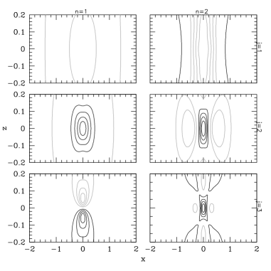
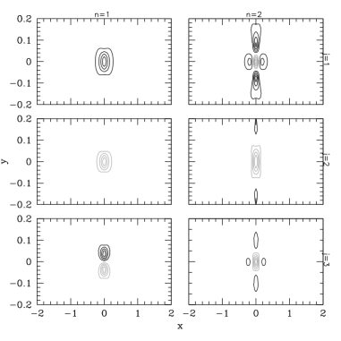
Figure 3: Cylindrical basis set conditioned by an exponential radial density profile and sech-squared vertical profile for $m=0$. The potential (density) members are shown on the left (right) labeled by radial and vertical orders. Positive (negative) isovalues are shown as black (gray).

Figure 3 shows the basis set for the SL method conditioned by an exponential radial density profile and $\mathop{\rm sech}\nolimits^{2}$ vertical profile. The steps in the construction were as follows:

1. The radial SL equation is solved numerically with conditioning functions $\Psi_{o}(R)\propto(1+(R/a)^{2})^{-1}$ and $\rho_{o}\propto\exp{-R/a}$. The vertical functions are sines and cosines with vacuum boundary conditions.

2. Linear combinations of the resulting eigenfunctions are found using an empirical orthogonal function analysis to find the best description of the $\Psi_{o}(R)\mathop{\rm sech}\nolimits^{2}(z/h)$ in the least squares sense.

3. The resulting basis functions are tabulated and interpolated as needed. Note that the basis can be chosen to have definite parity which optimizes table storage.

2.6 What good is all of this?

So far, we have explored a general approach for representing the gravitational potential for an ensemble of particles using particular harmonic bases. These bases can be derived in any coordinate system in which the Poisson equation is separable; at the very least, this includes all conic coordinate systems. Other advantages include:

• This potential solver is fast: it is ${\cal O}(N)$ with small coefficient. Recall that the most popular approaches: tree and grid codes are ${\cal O}(N\ln N)$. Direct summation is ${\cal O}(N^{2})$. For large $N$, this method has optimal scaling.

• Each term in the expansion resolves successively smaller structure. By truncating the series at the minimum resolution of interest or when the coefficients have low S/N, the high-frequency fluctuations are filtered out. This approach results in a relatively low-noise simulation; the high-frequency part of the noise spectrum dominates the particle noise in the standard potential solvers.

• Note that all of the dynamical information in a simulation is represented by the expansion coefficients. In other words, the expansion coefficients significantly compress the structural information in the simulation. If the dynamical content of the density and potential fields is the goal, one does not need to keep entire phase space, only the coefficients. Similarly, velocity fields may be represented by a similar expansion (e.g. [Saha 1993]).

• One is not restricted to individual components or single bases and can assign parts of phase space to separate bases depending upon its geometry or history. This is precisely what one needs to study a disk embedded in a spheroid and halo.

There is no one method for solving the Poisson equation in a simulation. The major disadvantages of the expansion approach is its lack of spatial adaptivity. It efficiently resolves non-axisymmetric features and disturbances as long as the galaxy does not change its structure rapidly. The approach is not highly adaptive and would not be good for equal mass merger, for example. Similarly, these schemes (like most efficient algorithms) do not strictly conserve momentum. In the limit of a large number of bodies, the expansion center is arbitrary because the distribution can be represented in an origin independent way regardless of the expansion center. For a smaller number of bodies, the number of available high-signal-to-noise ratio coefficients is too small to permit resolving the expansion about an arbitrary origin. The offset of the origin allowed for a given error bound decreases for with particle number. This demands that an efficient implementation of the expansion-based Poisson solver recenter the particle distribution.

These advantages, properties and limitations motivate a set of ideal applications:

1. Simulating a multicomponent galaxy. A feature of n-body simulation of galaxies is the disparate length scales of the disk, bulge and halo. This is not a problem for the expansion. We can pick a separate basis tailored to each component and determine the total gravitational field from their sum.

2. Long-term evolution. For a fixed number of particles, Poisson fluctuations and the simulation’s self-gravitating response to those fluctuations limit the length of time ${\cal T}$ that the evolution remains a good approximation to collisionless Boltzmann equation. For too few particles, the fluctuations can be so large that the angular momentum and energy of a particle orbit can drift or diffuse significantly over a single orbital time. Because the expansion method filters the high-frequency noise by construction, this is likely to give the largest value of ${\cal T}$ in most cases.

3. Weak, cumulative and tidal interactions. Similarly, this method is ideal for studying the response of a simulated galaxy to external global distortions. The scale sensitivity can be manipulated to efficiently represent the scales of interest and no others. Of course, limiting the resolution a priori is not always the best policy and this strategy must be motivated by a prior study with weaker constraints.

4. Stability. This Poisson solver is ideally suited to studying global stability. A time-series analysis of the coefficients can empirically yield both the growth rate and shape of the unstable mode.

3 A numerical method for perturbation theory

N-body simulation is not the only use for this special Poisson-solving biorthogonal expansion. We can exploit the completeness property to transform a linearized solution of the collisionless Boltzmann equation to a system of linear equations. This has been given the moniker matrix method by dynamicists but is a standard approach to solving partial differential equations [Courant and Hilbert 1953]. By using the same expansion for both an analytic linear solution and an n-body simulation, we explore a particular problem both ways and even apply the two together in various hybrid ways to further increase the dynamic range or time scale ${\cal T}$. I will sketch the development in the next section and follow this with a simple but complete example based on the slab model.

3.1 Introduction

The response of our stellar galaxy to any distortion is mathematically described by the simultaneously solution of the collisionless Boltzmann and Poisson equations:

$${\partial f\over\partial t}+{\partial H\over\partial{\bf p}}\cdot{\partial f\over\partial{\bf x}}-{\partial H\over\partial{\bf x}}\cdot{\partial f\over\partial{\bf p}} = 0,$$ (21)

$$\nabla\Phi({\bf x})=4\pi G\rho({\bf x}).$$ (22)

The steps in the solution are as follows. First we linearize equation (21) and note that equation (22) is already linear. We then separate the partial equations in their natural bases. In general, the two equations separate different bases and this presents a technical problem but not an insurmountable one. The Cartesian coordinate system is the exception: the bases are the same.

For a spherical stellar distribution, the biorthogonal potential-density pairs take the following form: $\Phi({\bf r})=\sum_{lm}\sum_{i}a^{lm}_{i}Y_{lm}(\theta,\phi)\Phi^{lm}_{i}(r)$ with an analogous expression for $\rho({\bf r})$. The two partial differential equations are then transformed to Fourier space using these bases to yield a set of algebraic equations. To do this, we note that orbits are quasi-periodic in regular potential. If all conserved quantities exist then by the averaging principle [Arnold 1978], we can represent any phase-space quantity by the following expansion in action and angles:

$$f({\bf p},{\bf x})=\sum_{\bf l}f_{\bf l}({\bf I})\exp(i{\bf l}\cdot{\bf w}).$$ (23)

If the gravitational potential admits chaotic orbits, this approach does not apply strictly. If the Lyapunov exponents are small, quasi-periodicity should still be a good approximation. With these tools and conditions, we begin by linearizing the collisionless Boltzmann equation (eq. 21). After expressing all phase-space variables in actions and angles, a Fourier transform in angles followed by a Laplace transform in times yields the solution

$${\hat{f}}_{1\,{\bf l}}({\bf I})={i{\bf l}\cdot{\partial f_{o}/\partial{\bf I}}\over s+i{\bf l}\cdot{\bf\Omega}}{\hat{H}}_{1\,{\bf l}}$$ (24)

where the hat denotes a Laplace transformed quantity and the subscript ${\bf l}$ denotes an action-angle transform. Finally, we can integrate equation (24) over ${\bf v}$ to get ${\hat{\rho}}_{1}({\bf I},{\bf w})$. We have not included the simultaneous solution of the Poisson equation but at this point, we tie the two together by expanding both ${\hat{\rho}}_{1}({\bf I},{\bf w})$ and the perturbing potential in the biorthogonal series. Explicitly, we can determine the scalar product of the potential component of the pair with the velocity integral of equation (24):

$$\int drr^{2}\Phi^{lm}_{i}(r){\hat{\rho}}_{1}({\bf I},{\bf w})=\int drr^{2}\Phi^{lm}_{i}(r)\int d^{3}v{i{\bf l}\cdot{\partial f_{o}/\partial{\bf I}}\over s+i{\bf l}\cdot{\bf\Omega}}{\hat{H}}_{1\,{\bf l}}.$$ (25)

The left-hand side is density expansion coefficients ${\bf a}$. The right-hand side may be written as the action of matrix on the vector of coefficients describing the perturbing potential ${\bf b}$. The matrix ${\cal R}$ depends on the underlying unperturbed distribution function and the Laplace expansion frequency $s$. In other words, the resulting solution for the response ${\bf a}$ given the perturbation ${\bf b}$ takes the form ${\bf a}={\cal R}(s){\bf b}$ for We may straightforwardly include the self-gravity in the response by noting the a self-gravitating response is the simultaneous solution of the system to both the perturbation and the response of the system to its own response. Mathematically, this is ${\bf a}={\cal R}(s)\left({\bf a}+{\bf b}\right)$ which upon solving for ${\bf a}$ yields ${\bf a}=\left[{\bf 1}-{\cal R}(s)\right]^{-1}{\cal R}(s){\bf b}$

Note our accomplishment: we began with a coupled set of partial-integrodifferential equations and end up with a matrix inversion. The computational work is all in determining the matrix elements of ${\cal R}$. Finally, after solving these sets of linear equations, we perform an inverse transform to obtain the resulting response to the perturbation in physical space.

I feel that the name matrix method is a bit of a misnomer, or at least not fully descriptive. The procedure described above has simple intuitive interpretation and this be even more apparent as we proceed through the next example. In transforming to Fourier space, we are in essence solving for the spectrum of normal modes of the system. The perturbation picks out the discrete modes and excites “packets” of continuous modes. After transforming back to physical space, we see the result of the decaying (or growing) discrete modes and phase-mixing packets of continuous modes in configuration space. In this sense, this approach might be more aptly called stellar spectral dynamics.

3.2 Example: slab dispersion relation

In this section, we apply this spectral dynamics approach to stellar slab described in §2.3.1. The natural coordinates here are Cartesian. The canonical variables describing the phase space are linear position and momentum in the slab and action-angle variables in the vertical direction. This simple case differs from a disk or halo in that trajectories are not bound in the two in-plane dimensions. Similarly, there is symmetry in the two in-plane dimensions so with no loss of generality we are free to consider only one of these, say the $x$ degree of freedom. So, the canonical variables are linear momentum and position ($p_{x},x$) and vertical action and orbital angle ($I_{z},\theta$). Orbital angle is defined as:

$$\theta=\Omega_{z}\int^{t}_{0}dt=\Omega_{z}\int^{z}_{0}{dz\over\sqrt{2(E_{z}-\Phi(z))}}$$

where $E_{z}$ is the energy in the vertical degree of freedom and $\Omega_{z}(E_{z})={\partial H/\partial I_{z}}$. The density and potential of the unperturbed equilibrium model does not vary in the infinite horizontal plane so the unperturbed quantities—density, potential and phase-space distribution function—do not vary in this dimension. This presents a formal difficultly popularized by Binney & Tremaine as the “Jeans’ swindle”. We will side step the subtleties here but please see Binney & Tremaine (1987) for discussion. We can now write our linearized equations of motion, the CBE and Poisson equation in these variables:

$${\partial f_{1}\over\partial t}+{\partial f_{1}\over\partial\theta}\Omega_{z}(E_{z})+{\partial f_{o}\over\partial x}p_{x}-{\partial f_{o}\over\partial E}\,{\partial V_{1}\over\partial\theta}\Omega_{z}(E_{z})-{\partial f_{o}\over\partial p_{x}}{\partial V_{1}\over\partial x}=0,\quad\nabla^{2}V_{1}({\bf r})=4\pi G\rho_{1}({\bf r}).$$ (26)

We now perform the two transforms: Fourier in actions and angles and Laplace in time. Again, the infinite horizontal extent causes a slight complication: a continuous set of plane waves rather than a discrete set that would obtain from a bound system. Let us denote the Fourier wave vector in the $x$ direction as ${\bf k}$, the index of the discrete vertical set as $n$ and the Laplace variable as $s$. A tilde indicates a Laplace transformed quantity. The transformed CBE becomes

$$s{\tilde{f}}_{1\,n{\bf k}}+in\Omega_{z}{\tilde{f}}_{1\,n{\bf k}}+i{\bf k}\cdot{\bf p}{\tilde{f}}_{1\,n{\bf k}}-{\partial f_{o}\over\partial E_{z}}\,in{\tilde{V}}_{1\,n{\bf k}}\Omega_{z}-{\partial f_{o}\over\partial E_{x}}\,i{\bf k}\cdot{\bf p}{\tilde{V}}_{1\,n{\bf k}}=0.$$ (27)

Solving for ${\tilde{f}}$, we now integrate over velocities to derive the Laplace-transformed density for each wave vector and vertical index. Integrating over wave vectors and summing over vertical indices gives us the expression for the response density for each Laplace frequency $s$:

$${\tilde{\rho}}({\bf r},s)=\sum_{n^{\prime}}\int d^{3}k^{\prime}\int d^{3}v\,{\tilde{f}}_{n^{\prime}\,{\bf k}^{\prime}}e^{in^{\prime}\theta(z)}e^{i{\bf k}^{\prime}\cdot{\bf R}}.$$ (28)

Next, we incorporate the Poisson equation by expanding the density and potential distortions in the biorthogonal functions in canonical variables::

$$p_{\mu\,{\bf k}}={1\over 2\pi}\ e^{i{\bf k}\cdot{\bf R}}\sum_{n}w_{\mu\,n}e^{in\theta}\hbox{\rm\ \ where\ \ }w_{\mu\,n}\equiv{1\over 2\pi}\int_{0}^{2\pi}d\theta\,\Psi_{\mu}(z)e^{-in\theta}.$$ (29)

Using the biorthgonality condition we perform the scalar product with equation (28) to get an linear set of equations that determine the expansion coefficients

$$a_{\,\mu{\bf k}}=-4\pi G\int d^{3}x\,d^{3}v\,p_{\mu\,{\bf k}}^{\ast}{\tilde{f}}_{n\,{\bf k}}e^{in^{\prime}z}e^{i{\bf k}^{\prime}\cdot{\bf R}}.$$ (30)

Substituting the solution for ${\tilde{f}}$, we have explicitly

$$a_{\mu\,{\bf k}}=-4\pi G(2\pi)\sum_{n,\nu}\int dv_{x}\,dv_{y}\int dI_{z}\,{\,{\partial f_{o}/\partial E_{z}}\,n\Omega_{z}+{\bf k}\cdot{\bf p}\,{\partial f_{o}/\partial E_{x}}\over n^{\prime}\Omega_{z}+{\bf k}\cdot{\bf p}-is}w_{\mu\,n}w_{\nu\,n}\,b_{\nu\,{\bf k}}$$ (31)

which can be written as the following matrix equation

$$a_{\mu\,{\bf k}}\equiv\sum_{n}\sum_{\nu}M^{n}_{\mu\nu}(s)\,b_{\nu\,{\bf k}}$$ (32)

To get the full self-gravitating response, we note that the imposed perturbation is then the sum of the internal response and external perturbation as follows:

$$a_{\mu\,{\bf k}}=\sum_{n}\sum_{\nu}M^{n}_{\mu\nu}(s,{\bf k})\,\left(a_{\mu\,{\bf k}}+b_{\nu\,{\bf k}}\right).$$ (33)

The solution for the response is then

$$a_{\mu\,{\bf k}}=\left[1-M^{n}_{\mu\alpha}\right]^{-1}{\cal M}_{\alpha\nu}b_{\nu\,{\bf k}}={\cal D}_{\mu\alpha}^{-1}{\cal M}_{\alpha\nu}b_{\nu\,{\bf k}}.$$ (34)

Alternatively, we can look for the perturbation that has the same shape as its own response, an eigenmode. The equation for this solution takes the form: $a_{\mu\,{\bf k}}={\cal M}_{\mu\nu}a_{\nu\,{\bf k}}$. A non-trivial solution demands that ${\cal D}(s)\equiv\det\{{\bf 1}-{\cal M}_{\mu\nu}(s)\}=0$ and this is often called the dispersion relation by analogy with the same relation that defines the possible wave modes in a plasma. We can classify the resulting modes by the real part of $s$. If $\mbox{Re}\,(s)>0$, $\mbox{Re}\,(s)=0$ and $\mbox{Re}\,(s)<0$, the mode is growing, oscillatory and damped, respectively. If we are interested in the evolution of a stable system, growing modes should be absent from the spectrum by design. Oscillatory modes are rare, requiring pattern frequencies which avoid commensurabilities with an integer combination of orbital frequencies. For reason, pure oscillating modes are practically non-existent, although one can construct special cases theoretically. The damped part of the spectrum has analogy with Landau damping in a plasma. Physically, the damping results from resonant transfer between the pattern and commensurabilities with orbital frequencies.

Note that all of these solutions are in Laplace space. To recover the time evolution, we must perform the inverse Laplace transform. This requires a bit of care but is straightforward (see the standard plasma literature, e.g. Krall & Trivelpiece, 1973 or Ikeuchi & Nakamura 1974 for details).

Finally, let us evaluate the response explicitly for a specific case. Recall that we are assuming that Let ${\bf{\hat{e}}}_{k}$ is ${\bf{\hat{e}}}_{x}$. Let us further assume that we can factor the phase-space distribution function as: $f_{o}(z,{\bf v})=f_{\parallel}(v_{x},v_{y})f_{\perp}(z,v_{z})$ Let the in-plane part of the distribution function be Maxwellian and the vertical part be be that for the $\mathop{\rm sech}\nolimits^{2}(z/h)$ density profile. The matrix elements $M^{n}_{\mu\nu}(s,{\bf k})$ now take the form

$$M^{n}_{\mu\nu}(s,{\bf k})=-4\pi G(2\pi)\int dI_{z}\,\int dv_{x}{\,{\partial f_{\perp}/\partial E_{z}}\,n\Omega_{z}-kv_{x}/\sigma^{2}f_{\perp}\over n^{\prime}\Omega_{z}+{\bf k}\cdot{\bf p}-is}{e^{-v_{x}^{2}/2\sigma^{2}}\over\sqrt{2\pi\sigma^{2}}}w_{\mu\,n}w_{\nu\,n}$$ (35)

Conveniently, the integrals over $v_{x}$ can be written as error functions of complex argument using the relation

$$\int^{\infty}_{-\infty}dv{e^{-v^{2}/2\sigma^{2}}\over kv+q}={1\over k}\int^{\infty}_{-\infty}dy{e^{-y^{2}}\over y+z}=-\pi i\mathop{\rm erf}\nolimits(-iz)e^{-z^{2}}$$ (36)

where $z=(n\Omega_{z}-is)/k\sqrt{2\sigma^{2}}$. Routines for evaluating the complex error function are readily available (e.g. www.netlib.org). Now let’s look at a few applications.

3.3 Modes in the slab

Modes are at the zeros of ${\cal D}$ which is shown in Figure 4. The figure only shows the dispersion relation as a function of $\omega\equiv-is$ rather than $s$. For reference, $\mbox{Im}\,(\omega)>0$ corresponds to instability. The dispersion relation is even in $\mbox{Re}\,(\omega)$ an exploration of the half-plane $\mbox{Re}\,(\omega)>0$ is sufficient. We see two zeros. The first has $\mbox{Im}\,(\omega)<0$ and very small $|\mbox{Im}\,(\omega)|\ll 1$. This is a damped mode but very weakly damped. The second, with larger $\mbox{Re}\,(\omega)$ is also weakly damped more strongly that the first.

Figure 4: Left: Plot of the dispersion relation $|D(\omega)|$ for the slab with a Maxwellian and sech-squared distribution. Center: odd mode (bending) and right: Even mode (Jeans).

To get physical intuition for these modes, one can can determine the shape of the mode by finding the null vector of $M^{n}_{\mu\nu}(s,{\bf k})$ for each zero in Figure 4. The two modes are shown also in Figure 4. The most weakly damped of the two is odd about the mid plane and is a traveling bending mode. The second mode mode is even about the mid plane and is a breathing mode. The dispersion relation ${\cal D}$ is also a function of $k$. The zeros ${\cal D}$ determine a branch for each mode. In this case, the damping increases as $|k|$ increases.

3.4 Excitation of a damped mode by a disturbance

We can use the information about the various modes in the dispersion to compute the excitation of the system due to a time-dependent disturbance. For example, let us consider the response of the slab due to a body passing through the slab at constant velocity. This is an idealization of a dwarf satellite moving through the disk (e.g. Sgr dwarf and the Milky Way).

We assume that we known time dependent of disturbance to start. After expanding this in our chosen biorthogonal basis, we can write this as vector of time-dependent of coefficients. The Laplace transform of the perturbation vector is then

$${\bf b}(s)=\int^{\infty}_{0}dt^{\prime}\exp(-st^{\prime}){\bf b}(t^{\prime})$$ (37)

The inverse Laplace transform of equation (31) gives

$${\bf a}(t) = {1\over 2\pi i}\int^{c+i\infty}_{c-i\infty}ds\,e^{st}{\cal D}_{\mu\alpha}^{-1}(s,{\bf k}){\cal M}_{\alpha\nu}(s,{\bf k})\int^{\infty}_{0}dt^{\prime}\exp(-st^{\prime}){\bf b}(t)$$ (38)

$$= \int^{\infty}_{0}dt^{\prime}{\bf b}(t^{\prime}){1\over 2\pi i}\int^{c+i\infty}_{c-i\infty}ds\,e^{s(t-t^{\prime})}{\cal D}_{\mu\alpha}^{-1}(s,{\bf k}){\cal M}_{\alpha\nu}(s,{\bf k})$$

The Laplace transform was performed assuming a value of $s$ that insured convergence. We are free to deform the integral path as long as we use care to analytically continue the integrand and identify singularities. In particular, if the slab is dynamically stable, then ${\cal D}$ is non-singular in the half plane with $\mbox{Re}\,(s)>0$. There will be poles for $\mbox{Re}\,(s)<0$ corresponding to damped modes. In addition, the matrix elements ${\cal M}$ have denominators of the form $s+ix$ for $x$ on the real line. The contour deformation rules are then: (1) for $t<t^{\prime}$, deform to $\mbox{Re}\,(s)\rightarrow\infty$, no poles; and (2) for $t>t^{\prime}$, deform to $\mbox{Re}\,(s)\rightarrow-\infty$, poles at $s=-ix$ and at any possible poles of ${\cal D}$ in the lower-half $s$-plane (damped modes). Performing the inverse Laplace transform and putting everything together gives the explicit expression for the self-gravitating time-dependent response to the perturbation:

$${\bf a}(t) = -4\pi G(2\pi)\int dI_{z}\,\int dv_{x}\,i\left({\partial f_{o}\over\partial E_{z}}\,n\Omega_{z}+kv_{x}{\partial f_{o}\over\partial E_{x}}\right)\times$$ (39)

$${\cal D}_{\mu\alpha}^{-1}(-ix,{\bf k})w_{\mu\,n}w_{\nu\,n}\int^{\infty}_{0}dt^{\prime}{\bf b}(t^{\prime})e^{-ix(t-t^{\prime})}+$$

$$\sum_{s_{r}}\mathop{\rm Res}\nolimits{\cal D}_{\mu\alpha}^{-1}(s_{r},{\bf k}){\cal M}_{\alpha\nu}(s_{r},{\bf k})\int^{\infty}_{0}dt^{\prime}{\bf b}(t^{\prime})e^{s_{r}(t-t^{\prime})}$$

The inverse of the dispersion matrix will have poles at any modes (recall Cramer’s formula). The notation $\mathop{\rm Res}\nolimits{\cal D}_{\mu\alpha}^{-1}$ denotes the residue of the this matrix and may be determined numerical using singular value decomposition with the following procedure: (1) locate the damped modes $s_{r}$ and compute ${\cal D}_{\mu\nu}(s_{r})$; (2) analyze by singular value decomposition and compute the determinant without the singular value, $D\prime(s_{r})$ say; (3) compute the derivative of the determinant at $s_{r}$, $dD/ds|_{s_{r}}$. We expect $D(s)=a(s-s_{r})D^{\prime}(s_{r})$ for some unknown constant of proportionality whose solution is: $a=dD/ds|_{s_{r}}/D^{\prime}(s_{r})$; and (4) replace the singular value in the decomposition by the value of $a$. I have given explicit details for readers interested in exploring this procedure numerically. The numerical computations here are straightforward for this case of the slab. One should be able to investigate the full response of the slab to an arbitrary perturbation.

4 Galaxy interactions

Let us finish with examples of these methods applied to two classes astronomical scenarios. First, we will mention the excitation of structure by a passing galaxy such as a weak encounter in group, a fly-by. These interactions can cause off-centered disks and centers and trigger bars. Similarly, an orbiting satellite will have a very similar effect on its primary. Second, we will describe noise-driven evolution, both the shape and magnitude of fluctuation-driven structure and the possibility of significant evolution of halo profiles due to these fluctuations.

4.1 Fly-bys and satellites

Another way of getting the same sort of excitation, perhaps more important for group galaxies than the Milky Way, is a passing fly-by. A perturber on a parabolic or hyperbolic trajectory can excite similar sorts of halo asymmetries and persist until long after the perturber’s existence is unremarkable. Presumably, our Galaxy has suffered such events in the past but because the satellite excitation is closely related to the fly-by excitation, the study of one will provide insight into the other. Vesperini & Weinberg [Vesperini and Weinberg 2000] describes the application of the response approach to this problem. From these analytic calculations, we can compute the standard asymmetry parameters [Abraham et al. 1996b, Abraham et al. 1996a, Conselice et al. 2000] obtained by summing over the mean square difference of the galaxy and its $180^{\circ}$ rotated image:

$$A={1\over 2}{\sum\left|I(x,y)-I_{rot}(x,y)\right|\over\sum I(x,y)}.$$ (40)

For example, a perturber with 10% of the halo mass, with pericenter at the halo half-mass radius, and encounter velocity of 200 km/s will produce $A\approx 0.2$. Damped modes play a major role in both the morphology and longevity of these modes. Figures 6 and 7 in Vesperini & Weinberg (2000) illustrates their importance by comparing the response with and without damped modes. The $m=1$ mode is significantly altered by the discrete weakly damped mode. Please see [Vesperini and Weinberg 2000] for more details.

Because the halo response is dominated by the modes of the halo rather than properties of the perturber, we expect that the asymmetry should be dominated by contributions at well-defined radii, independent of the perturber parameters. We proposed a simple generalization of equation (40) to test this prediction: define $A(r)$ to be the sums over pixels restricted to those within projected radius $r$. More recently, we have shown that n-body simulations agree in magnitude and morphology with the perturbation theory.

4.2 Noise

The possibility of long-lived damped modes leads to the possibility that global modes are continuously excited by a wide variety of events such as disrupting dwarfs on decaying orbits, infall of massive high velocity clouds, disk instability and swing amplification and the continuing equilibration of the outer galaxy. The dominant halo modes are low frequency and low harmonic order and therefore can be driven by a wide variety of transient noise sources. Some recent work [Weinberg 2000b, Weinberg 2000a] provides a theory excitation by noise and applies this to the evolution of halos. In this section, I will first describe an application of our response theory to fluctuation noise. I will describe some preliminary results suggest that noise may drive a halos toward approximately self-similar profiles. Additional work will be required to make precise predictions for these trends and explore the consequences for long-term evolution of disks in spiral systems.

4.3 Halo noise

The simplest approach is a calculation of the power in a stellar system due to Poisson fluctuations. Consider the response of the entire system to a single orbiting star. Physically, each star excites a wake in the halo. This wake includes all the modes from the weakly damped modes to very small scale modes. We now sum up the wakes from all of the stars. The self-gravity of the lowest-order mode leads to significant excess power at large scales. The detailed theoretical computation is compared with n-body simulations in Figure 5. Note that the amplification of the noise by self-gravity is significant for the $l=1$ component for both halos with and without cores.

Figure 5: Power (in energy units) of the response of a halo to noise for two different models as a function of radial basis index. Left: $W_{0}=5$ King model. Right: Hernquist model. The top row left (right) shows the $l=1$ ($l=2$) response for each model. The bottom row shows the cumulative power. The radial basis set is similar to that shown in Fig. 2; the index on the abscissa indicates the number of nodes for each basis function. The larger the index, the finer the spatial scale.

The analytic calculation is valid in the limit $N\rightarrow\infty$. However, if this is not obtained in the n-body simulation, the power in fluctuations can be so large that individual orbits do not have well-defined conserved quantities (energies and angular momenta) over a dynamical time. In this noise-dominated regime, the diffusion of orbits is so fast that coherent large-scale dynamics is suppressed. In other words, with too few particles, one is simulating a star cluster not dark-matter dominated halo. We can see the effects of particle number by determining the number $N$ required to obtain the noise-spectrum predicted by analytic solution of the underlying power spectrum. This is illustrated in Figure 6. The figure compares same empirically determined power spectra shown in Figure 5 (left panel) but for various values of $N$. In short, one needs $N\geq 10^{6}$ before the dynamics of the collisionless limit obtains. This result is largely independent of the n-body simulation technique.

Figure 6: Left: Fluctuation power as a function of particle number for each basis coefficient scaled by the number of particles $N$. Right: Fluctuation power for $n=5$ as a function of particle number. The upper (lower) horizontal lines show the expected results with self gravity (Poisson).

4.4 Evolution of galaxy by noise

Given that fluctuations are a generic part of stellar dynamics, let us know ask what sort of evolution we can expect. To do this, I will sketch the development of a constitutive equation for the long-term evolution under noise. We could proceed as for globular clusters: expand the Boltzmann collision term using Master formalism [Binney and Tremaine 1987]. After a number of false starts, I found the more general transition probability approach to be more natural (although the Master approach is formally equivalent). One begins with the probability that an orbit with phase-space state ${\bf x}$ at time $t$ makes a transition to ${\bf x}^{\prime}$ at time $t+\tau$: $P({\bf x}^{\prime},t+\tau|{\bf x},t)$. For the entire ensemble described by the distribution function $f({\bf x},t)$, we can describe the evolution using the transition probability as

$$f({\bf x},t+\tau)=\int d{\bf x}^{\prime}P({\bf x},t+\tau|{\bf x}^{\prime},t)f({\bf x}^{\prime},t).$$ (41)

Now, expand the transition probability in its moments of ${\bf x}-{\bf x}^{\prime}$ for small $\tau$. This gives

$${\partial f({\bf x},t)\over\partial t}=\sum_{n=1}^{\infty}\left(-{\partial\over\partial{\bf x}}\right)^{n}D^{(n)}({\bf x},t)f({\bf x},t)$$ (42)

This is known as the Kramers-Moyal expansion[Risken, 1989].

We will derive the transition probability for our case by considering the change in conserved quantities of orbits (actions) over the correlation time of the fluctuation. This implies that the transition probability is only defined for time scales $\tau$ larger than the dynamical orbital time scales. Therefore, we can further simplify the computation by using action-angle variables and averaging over the rapidly varying angles. For the phase-space distribution function, the Kramers-Moyal expansion becomes

$$f({\bf I},t+\tau)=\int d{\bf I}^{\prime}\,P({\bf I},t+\tau|{\bf I}^{\prime},t)f({\bf I}^{\prime},t)$$ (43)

Now to evaluate this equation, expand integrand in a Taylor series about ${\bf I}$ and define $\Delta\equiv{\bf I}^{\prime}-{\bf I}$. In the limit $\tau\rightarrow 0$, we

$${\partial f({\bf I},t+\tau)\over\partial t}=\sum_{n=1}^{\infty}\left(-{\partial\over\partial{\bf I}}\right)^{n}D^{(n)}({\bf I},t)f({\bf I},t).$$ (44)

where $D^{n}$ is proportional to the time-derivative of the moments of $\Delta$ over the distribution $P$. However, despite the appearance of continuous functions in these formulae, note that $P$ describes stochastic events. To write this explicitly in stochastic variables, let ${\bf\xi}$ be the stochastic value of ${\bf I}$. The expression $D^{(n)}$ may be written

$$D^{(n)}(x,t)=\left.{1\over n!}\lim_{\tau\rightarrow 0}{1\over\tau}\langle[{\bf\xi}(t+\tau)-{\bf I}]^{n}\rangle\right|_{{\bf\xi}(t)={\bf I}}.$$ (45)

If stochastic excitation is a Markov process, this guarantees that the expansion terminates after two terms [Pawula 1967]. Our evolution equation is then a Fokker-Planck equation:

$${\partial f({\bf I},t)\over\partial t}=\left\{-{\partial\over\partial{\bf I}_{i}}D^{(1)}_{i}({\bf I},t)+{\partial^{2}\over\partial{\bf I}_{i}\partial{\bf I}_{j}}D^{(2)}_{ij}({\bf I},t)\right\}f({\bf I},t).$$ (46)

4.5 Noise-dominated halo evolution

To end this section, we will describe the application of this formalism to the long-term evolution of a halo under a several representative noise processes.

First, some general observations. Noise from periodically orbiting bodies do not give rise to long-term evolution, even though they do give rise to significant orbital diffusion (as described above). This is easily argued. Changes over long time periods, so-called secular changes, will only occur if the disturbance presents a torque. Consider the mean density of an orbiting body over many dynamical times, for example. It will only present a torque if it is a closed, resonant orbit. At order $l=1$, this requires that the radial and azimuthal frequencies be equal, as in a Keplerian orbit. For most halo profiles, these orbits populate the outer edge and therefore have little effect. Similarly, at order $l=2$, we add the possibility of closed, stationary bar-like orbits that have radial frequencies that are twice the azimuthal frequencies. This can occur in homogeneous cores, but these conditions are thought to be rare or non-existent in realistic halos. Order $l=3$ is the lowest order that admits resonant orbits over a wide-range of energies. This is not inconsistent with the the results of §4.2. Noise at orders $l=1,2$ caused by orbiting bodies can cause significant orbital diffusion without changing the equilibrium profile. This turns out to be a corollary of a more general proof of the stability of stellar equilibria against phase-mixing [Hjorth 1994]. Parenthetically, N-body folks have used the maintenance of an equilibrium as an indicator of the collisionless regime. However, the argument above shows that the equilibrium will persist even if the rate of orbital diffusion is high.

Conversely, any transience in the noise source—orbital decay, fly-bys, disrupting or shearing stellar streams—can excite the weakly damped modes at low order. Since a galactic halo will suffer all of these disturbances over its lifetime, direct numerical estimates suggest that excitation of transient noise will dominate orbital noise in driving evolution for realistic astronomical scenarios and I will give examples of these below [Weinberg 2000b, Weinberg 2000a].

The overall procedure is as follows. We begin with an equilibrium halo and phase-space distribution function. To simplify solution of the Fokker-Planck equation, the distribution is isotropized. The evolution equation (46) is now solved in two steps. First, we solve the Fokker-Planck equation holding the underlying gravitational potential fixed for some $\tau$ greater than $1/\Omega$ but small compared to overall evolution time scale. Second, we “turn off” the collision term and find new self-consistent equilibrium. The two-step process is repeated to obtain the evolution.

Figure 7 shows the evolution under three different noise sources: (1) a satellite with a decaying orbit; (2) a halo of black holes; and (3) satellite fly-bys. In the the first two cases, we begin with a $W_{0}=5$ King model and the third begins with a broken power-law profile (with a small core for numerical convenience). For Cases (1) and (3), the results can be characterized as follows. There are two distinct evolutionary phases: a transient readjustment to a double power law profile followed slow, approximately self-similarly evolution. The outer profile is characterized by power law with exponent close to $-3$. The profile continues to approach the $-3$ power-law form at increasing radius as the evolution continues. [Weinberg 2000a] shows that this obtains for a wide variety of initial conditions and is caused by the reaction of the halo to the external $l=1$ multipole, which explains the ubiquity of the profile. The inner profile has a shallower roll before reaching the core. A power law of -1.5 is shown for comparison. The more concentrated models, which have deeper potential wells and therefore shorter dynamical times, evolve most quickly. This is clear in the comparison of Cases (1) and (3) but [Weinberg 2000a] shows that this obtains for a variety of initial conditions. Case (2), evolution by orbiting black holes, does not result in the same asymptotic form and exhibits much weaker evolution overall.

Because these models have cores, and both the radial and azimuthal orbital frequencies are nearly the same in the core, it is difficult to couple to these orbits in order to transfer angular momentum in and out of the core. The core, then, expands with the overall expansion of the halo due to the deposition of energy from the noise sources. These dynamics suggest that we restrict our consideration to evolution beyond the core. Further investigation of the importance of an initial cusp are in progress.

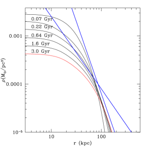
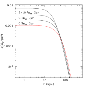
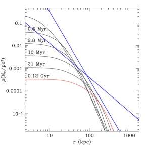
Figure 7: Left: Orbital decay in a $W_{0}=3$ King model halo for a satellite to halo mass ratio of 0.05. The straight lines are power laws with exponents $-1.5$ and $-3$, for comparison. Center: Evolution of a King $W_{0}=3$ profile under ‘black hole’ noise. The times for each curve are shown with the scaling for number of black holes per halo assuming that the black hole fraction is 10%. This gives roughly $n_{bh}=10^{6}$ and the evolution time scale is uninterestingly large. Right: Evolution for a double power law model $\rho\propto(r+\epsilon)^{-\gamma}(r+1)^{\gamma-\beta}$ with $\gamma=1$, $\beta=4$ and $\epsilon=0.1$.

5 Summary and topics for future work

These lectures have described the use of biorthogonal expansions in n-body simulations and perturbation theory to understand the long-term evolution of galaxies. For a concrete example, I presented an explicit example of an infinite slab which as a rich modal structure but can be treated analytically and by n-body simulation with a small amount of numerical computation.

One can use these same procedures with carefully chosen bases to represent gravitational field of galaxies to perform smooth, low-diffusion, n-body simulations. Multiple disk, bulge and halo components can be treated simultaneously by using separate bases for each component since solutions of Poisson equation are additive. The same expansion bases can be used to construct perturbation theories for understanding the stable and unstable modes and deriving the response to time-dependent disturbances. The advantage of using the perturbation theory is its insensitive to particle noise and resulting orbital diffusion which can wipe out correlations that critical to dynamics. Because both the n-body simulations and the perturbation can be represented by the same field expansion, the two approaches can be used together to understand the details of a complex interaction.

Using these methods, we have seen that many if not all astronomical equilibria have weakly damped modes. These modes easy to excite and slow to decay and therefore will tend to dominate the non-axisymmetric structure of galaxies. For example, the ubiquity of very weakly-damped “sloshing modes” ($l=m=1$) may cause lopsided disks, off-centered nuclei including nuclear bars and black holes. The basic dynamics here was throughly explored decades ago by the pioneers in spiral structure [Lin and Shu 1964, Julian and Toomre 1966, Toomre 1969, Shu 1970a, Shu 1970b]. In particular, global spiral structure was shown to be damped [Toomre 1969] for the same physical reasons.

We described several applications, satellite and fly-by induced lopsidedness and bars and excitation of structure by noise, emphasizing the latter. In particular, the Poisson noise from a simulation of a halo with $10^{5}$ particles drives enough power, when damped modes are included to cause observable disturbances in the disk. Physically, this noise is comparable to a halo of black holes of 2 to $6\times 10^{6}{\rm\,M_{\odot}}$. Conversely, one needs at least $10^{7}$ bodies to suppress the particle noise to the point that the collisionless limit is obtained with some confidence. We then considered the long-term consequences of this noise to the evolution of a galaxy halo. We argued that dwarf mergers, weak encounters with neighbors, and noise from the still equilibrating outer halo can drive significant halo evolution through noise excitation over a galaxy lifetime.

There is much more that needs to be done in this area, including careful analysis of more realistic galaxy models under a wide variety of possible perturbations and noise spectra. Calculations to date have only considered stellar dynamics, but the gas component response to the large-scale structure discussed here may prove important to our understanding of galaxy evolution as well as providing an important observational diagnostic. This all leads to the speculative possibility that galactic evolution may be driven by stochastic evolution, at least in part. It will be interesting to see if a stochastic view rather than static view is borne out.

References

References

- [Abraham et al. 1996a] Abraham, R. G., Tanvir, N. R., Santiago, B. X., Ellis, R. S., Glazebrook, K., and van den Bergh, S. 1996a, MNRAS, 279, L47.
- [Abraham et al. 1996b] Abraham, R. G., van den Bergh, S., Glazebrook, K., Ellis, R. S., Santiago, B. X., Surma, P., and Griffiths, R. E. 1996b, ApJS, 107, 1.
- [Arnold 1978] Arnold, V. I. 1978, Mathematical Methods of Classical Mechanics, Springer-Verlag, New York.
- [Binney and Tremaine 1987] Binney, J. and Tremaine, S. 1987, Galactic Dynamics, Princeton University Press, Princeton, New Jersey.
- [Clutton-Brock 1972] Clutton-Brock, M. 1972, Astrophys. Space. Sci., 16, 101.
- [Clutton-Brock 1973] Clutton-Brock, M. 1973, Astrophys. Space. Sci., 23, 55.
- [Conselice et al. 2000] Conselice, C. J., Bershady, M. A., and Jangren, A. 2000, ApJ, 529, 886.
- [Courant and Hilbert 1953] Courant, R. and Hilbert, D. 1953, Methods of Mathematical Physics, Vol. 1, Interscience, New York.
- [Dahlquist and Bjork 1974] Dahlquist, G. and Bjork, A. 1974, Numerical Methods, Prentice-Hall, Englewood Cliffs.
- [Hall 1981] Hall, P. 1981, Ann. Stat., 9, 683.
- [Hernquist 1990] Hernquist, L. 1990, ApJ, 356, 359.
- [Hernquist and Ostriker 1992] Hernquist, L. and Ostriker, J. P. 1992, ApJ, 386(2), 375.
- [Hjorth 1994] Hjorth, J. 1994, ApJ, 424, 106.
- [Ikeuchi et al. 1974] Ikeuchi, S., Nakamura, T., and Takahara, F. 1974, Prog. Theor. Phys., 52.
- [Julian and Toomre 1966] Julian, W. H. and Toomre, A. 1966, ApJ, 146, 810.
- [Kalnajs 1976] Kalnajs, A. J. 1976, ApJ, 205, 751.
- [Kalnajs 1977] Kalnajs, A. J. 1977, ApJ, 212(3), 637.
- [Krall and Trivelpiece 1973] Krall, N. A. and Trivelpiece, A. W. 1973, Principles of Plasma Physics, McGraw-Hill, New York.
- [Lin and Shu 1964] Lin, C. C. and Shu, F. 1964, ApJ, 140, 646.
- [Morse and Feshbach 1953] Morse, P. M. and Feshbach, H. 1953, Methods of Theoretical Physics, McGraw Hill, New York.
- [Pawula 1967] Pawula, R. F. 1967, Phys. Rev., 162, 186.
- [Pruess and Fulton 1993] Pruess, S. and Fulton, C. T. 1993, ACM Trans. Math. Software, 63, 42.
- [Risken, 1989] Risken, H. 1989, The Fokker-Planck Equation, Springer-Verlag.
- [Robijn and Earn 1996] Robijn, F. H. A. and Earn, D. J. D. 1996, MNRAS, 282, 1129.
- [Saha 1993] Saha, P. 1993, MNRAS, 262, 1062.
- [Shu 1970a] Shu, F. H. 1970a, ApJ, 160, 89.
- [Shu 1970b] Shu, F. H. 1970b, ApJ, 160, 99.
- [Toomre 1969] Toomre, A. 1969, ApJ, 158, 899.
- [Vesperini and Weinberg 2000] Vesperini, E. and Weinberg, M. D. 2000, ApJ, 534, 598.
- [Weinberg 1999] Weinberg, M. D. 1999, AJ, 117, 629.
- [Weinberg 2000a] Weinberg, M. D. 2000a, Noise-driven evolution in stellar systems: Theory, submitted to MNRAS, astro-ph/0007275.
- [Weinberg 2000b] Weinberg, M. D. 2000b, Noise-driven evolution in stellar systems: A universal halo profile, submited to MNRAS, astro-ph/0007276.