Jet stability and the generation of superluminal and stationary components

Abstract

We present a numerical simulation of the response of an expanding relativistic jet to the ejection of a superluminal component. The simulation has been performed with a relativistic time-dependent hydrodynamical code from which simulated radio maps are computed by integrating the transfer equations for synchrotron radiation. The interaction of the superluminal component with the underlying jet results in the formation of multiple conical shocks behind the main perturbation. These trailing components can be easily distinguished because they appear to be released from the primary superluminal component, instead of being ejected from the core. Their oblique nature should also result in distinct polarization properties. Those appearing closer to the core show small apparent motions and a very slow secular decrease in brightness, and could be identified as stationary components. Those appearing farther downstream are weaker and can reach superluminal apparent motions. The existence of these trailing components indicates that not all observed components necessarily represent major perturbations at the jet inlet; rather, multiple emission components can be generated by a single disturbance in the jet. While the superluminal component associated with the primary perturbation exhibits a rather stable pattern speed, trailing components have velocities that increase with distance from the core but move at less than the jet speed. The trailing components exhibit motion and structure consistent with the triggering of pinch modes by the superluminal component. The increase in velocity of the trailing components is an indirect consequence of the acceleration of the expanding fluid, which is assumed to be relativistically hot; if observed, such accelerations would therefore favor an electron-positron (as opposed to proton rest-mass) dominated jet.

1 Introduction

The computation of the synchrotron radio emission (Gómez et al. 1995, 1997; Hughes, Duncan & Mioduszewski 1996; Komissarov & Falle 1996) from time-dependent relativistic hydrodynamical codes (Martí, Müller, & Ibáñez 1994; Duncan & Hughes 1994; Koide, Nishikawa, & Mutel 1996) has proven to be a powerful method to understand the physics of jets in AGNs and microquasars improving upon previous idealized analytical calculations (Marscher & Gear 1985, Hughes et al. 1985). Superluminal components have been studied using such formulations by introducing perturbations in the jet inlet and analyzing the resulting shock waves and their subsequent evolution along the jet (Gómez et al. 1997; Mioduszewski et al. 1997). Fluctuations in the internal structure of the shocked material may be amplified by time delay effects, resulting in a knotty brightness distribution of the superluminal component associated with the shocked plasma (Gómez et al. 1997).

In this Letter we explore the instabilities produced in the jet resulting from the evolution of strong perturbations generated at the jet inlet. In particular, we describe a mechanism, which should be common in jets, that generates multiple superluminal as well as quasi-stationary components.

2 Generation of Traveling Perturbations in Relativistic Jets

Our study relies on a relativistic, axially-symmetric jet model obtained by means of a high-resolution shock capturing scheme to solve the equations of relativistic hydrodynamics in cylindrical coordinates. The code is the same as that used by Gómez et al. (1997). Details of the code and its performance (equations, finite–difference approximation, and testing) can be found in Martí et al. (1997, and references therein).

The steady jet model is the same as model PM in Gómez et al. (1997), computed with a spatial resolution in both radial and axial directions of 8 cells/$R_{b}$ (where $R_{b}$ is the beam radius at the injection position), but twice as long (covering 400x10 $R_{b}$). It corresponds to a pressure-matched, diffuse ($\rho_{b}/\rho_{a}=10^{-3}$), relativistic ($\Gamma_{b}=4$) beam with Mach number $M_{b}=1.69$. Here $\rho$ is the proper rest-mass density and $\Gamma$ is the bulk Lorentz factor; subscripts $a$ and $b$ refer, respectively, to atmosphere and beam; values correspond to the injection position. By allowing the jet to propagate through an isothermal atmosphere with a decreasing pressure gradient, we have induced a small opening angle in the jet ($\sim$ 0.3^∘).

2.1 Dynamics of the main perturbation

We concentrate our attention on the evolution of the flow after the introduction of a square-wave perturbation at the jet inlet. This perturbation consists of an increase in the bulk Lorentz factor from the quiescent value of $\Gamma_{b}=4$ to $\Gamma_{p}=10$, and an increase in pressure by a factor of two. The perturbation lasts for a time $\tau_{p}=0.75R_{b}/c$ (where $c$ is the speed of light), after which the jet inlet was set to the quiescent values both in Lorentz factor and pressure. The fluid piles up in front of the velocity perturbation, creating a fast shocked state. Given the large initial shock velocity of $\sim$0.995 ($\Gamma=10$), in order to determine relative variations in this velocity of the order of 10% (for example, to discern between a shock Lorentz factor of 10 and, say, 11), the relative error in the calculation of the distance traveled by the shock must be smaller than 1/1000. This precision can only be obtained by studying the evolution of the shock over more than 1000 computational cells. Given the fact that the shock front is spread over 3-4 cells and the computational domain covers 3200 cells, only mean shock speeds (of 0.995 $c$) can be obtained. In general, the Lorentz factor of the leading shock should be larger than that of the pre-shock flow ($\sim 4$ at $z=0$; $\sim 12$ at $z=400R_{b}$). This shocked state is followed by a more slowly moving (mean speed of 0.973 $c$) rarefaction where the fast flow separates from the slower upstream flow. This difference in speeds stretches the perturbation along the axis. Any similar strong supersonic perturbation should lead to a similar shock/rarefaction structure.

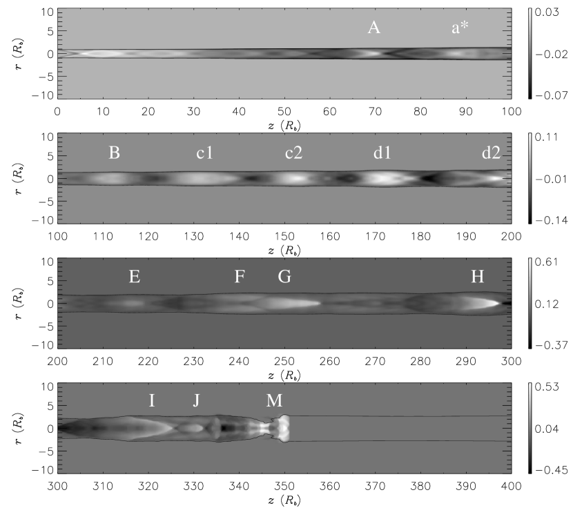
Figure 1: Relative variation with respect to the undisturbed steady jet of the Lorentz factor (logarithmic scale) at t=350 $R_{b}/c$. Note the different scale ranges in each frame to enhance the representation of the trailing conical shocks (labeled A to J) following the main perturbation (M). Typical shock angles to the jet axis are $\sim 10-15^{\circ}$.

The passage of the main perturbation triggers a local pinch instability that propagates behind the main perturbation, leading to the formation of a series of conical “trailing shocks” following the main perturbation (Fig. 1). Shocked and rarefied parts of the main perturbation and variation in the beam radius can be seen in the figure. The trailing structures are spaced by $\sim 8~{}R_{b}$ for $15<z/R_{b}<55$ and $\sim 20~{}R_{b}$ for $105<z/R_{b}<180$.

Although the type of perturbation introduced at the jet inlet is somewhat arbitrary, the qualitative results we obtain are not a function of the particular perturbation chosen; formation of trailing shocks is a general consequence of the propagation of strong perturbations through jets (see also Gómez et al. 1997, where trailing shocks appear in the hydrodynamical simulations for a different jet inlet perturbation). Further research would be of interest to quantify the physics of the trailing shocks depending on the type of perturbation introduced, as well as the jet/external medium hydrodynamical properties.

A local solution of the dispersion relation for the pinch modes of this relativistic jet and a computation of the pinch mode structure (see Hardee et al. 1998; Hardee 2000) indicate that observed features are primarily related to triggering of the first pinch body mode. Features in Figure 1 in the range $15<z/R_{b}<180$ have spacings between the longest unstable wavelength $\lambda^{\it l}$ and the shorter maximally unstable wavelength $\lambda^{*}$ of the first pinch body mode. The wavelengths $\lambda^{\it l}$ and $\lambda^{*}$ increase from 13 $R_{b}$ to 125 $R_{b}$ and from 4 $R_{b}$ to 19 $R_{b}$, respectively, as $z$ increases from 0 to 250 $R_{b}$.

2.2 Evolution of the Trailing Shocks

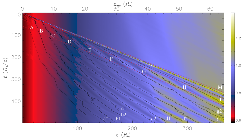
Figure 2: Space-time diagram for the logarithm of the jet Lorentz factor distribution. The diagonal black line from top left to bottom right marks the trajectory of the main perturbation (M), whereas the remaining black lines correspond to the tracks of the trailing shocks (identified as local maxima at positions where the Lorentz factor is 1% or more higher than the steady jet model). Red lines correspond to constant observer’s times $t_{obs}$=0, 30, and 60 $R_{b}/c$ for a viewing angle of $10^{\circ}$.

The observed time evolution of the trailing shocks can be followed in Figure 2, which displays a space-time diagram of the Lorentz factor distribution in the jet. Trailing shocks emerge from the rarefactions that follow the main perturbation, and are generated over a range of velocities and separations. The velocities are significantly smaller than the velocity of the main perturbation (and the bulk flow speed) and increase with distance from the inlet, as do the separations. Table 1 summarizes the positions, separations, and speeds of the trailing components for different observer’s times. In particular, consider time $t_{obs}=60$ when the shock spacing from A to H ranges from $\sim 17~{}R_{b}$ to $\sim 76~{}R_{b}$ and the shock velocity ranges from $\sim 0.13c$ to $\sim 0.69c$ for locations from $z/R_{b}=12.7$ to $z/R_{b}=290.9$. The separation and speed are explained by rapid passage of the main perturbation, which triggers the first pinch body mode at a wavelength whose group velocity is comparable to the rarefaction speed, $v_{gp}\sim 0.973~{}c$. This wavelength ranges from $\lambda\sim 23~{}R_{b}$ at $z/R_{b}\sim 50$ to $\lambda\sim 60~{}R_{b}$ at $z/R_{b}\sim 250$. Subsequently, the perturbation slows to the wave speed, $v_{ph}$, of this wavelength. The wave speed ranges from $\sim 0.2~{}c$ at $z/R_{b}\sim 50$ to $\sim 0.6~{}c$ at $z/R_{b}\sim 250$. The wave speed is low for perturbations created with wavelength near $\lambda^{\it l}$ (occurs at small $z$) and higher for perturbations created with wavelength above $\lambda^{\it l}$ (occurs at larger $z$). Another result is that perturbations created at small $z$ (relatively short wavelength) accelerate as they move to larger $z$ (see Fig. 2) where their wave speed is higher.

3 Emission results

We have computed the synchrotron radiation from the hydrodynamical model discussed in the preceding section following the procedure described in Gómez et al. (1997) and references therein. Fig. 3 shows the computed total intensity image obtained for an optically thin observing frequency. Several components are seen, corresponding to the trailing conical shocks of Figs. 1 and 2, and labeled accordingly. Typical high-frequency VLBI observations provide dynamic ranges of the order of 200:1 (defined as the intensity ratio of the peak to the lowest believable feature) or larger, depending on the frequency of observation and array used. All components seen in Fig. 3 are above this limit, and therefore are expected to be detected by actual VLBI observations.

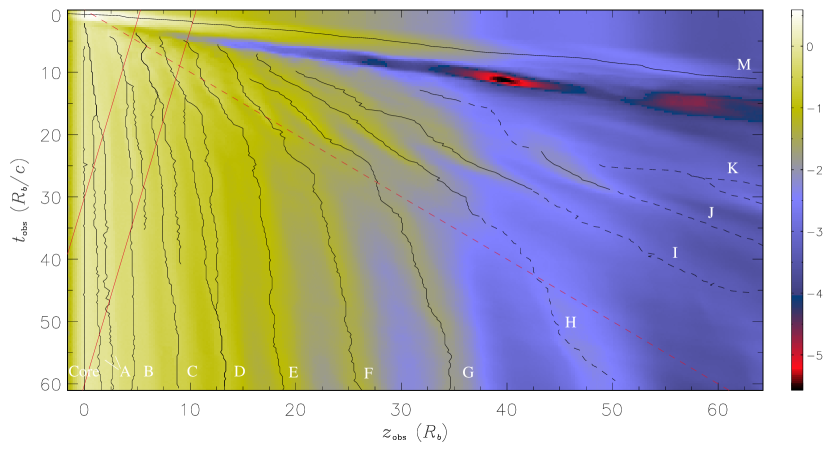
Figure 4: Space-time diagram for the logarithm of the mean (unconvolved) intensity (across slices normal to the jet axis and normalized to the mean core intensity) in the observer’s frame. Black tracks correspond to trajectories of emission components associated with the main perturbation (M) and the trailing components. Black dashed lines correspond to components with intensities below 0.5% of the normalized value. Red continous lines are lines of constant time in the source frame (from left to right, $t=30,60R_{b}/c$). The red dashed line represents a speed equal to $c$.

Figure 4 displays the mean intensity along the observed jet in a space-time diagram. Trailing components have been identified across epochs, and their mean intensity peak is traced as a function of observer’s time. Almost all the trailing shocks in Fig. 2 can be identified with radio components in Fig. 4 and have been labeled accordingly. In Fig. 4 we can distinguish a strong component associated with the main shock, followed by a jet region with low emission corresponding to the rarefaction that follows the main shock. Trailing components are observed to emerge upstream from this dip in emission. Therefore, trailing components can be easily distinguished from those generated at the jet inlet: they emanate not from the core, but rather seem to appear spontaneously downstream, created in the wake of strong perturbations. The main component is observed to move with a superluminal apparent speed that slowly decreases from $\sim 7$ to $\sim 6c$. Note that from these velocities we can infer a Lorentz factor for the hydrodynamical component between 7.3 and 6.1 (for a viewing angle of $\theta=10^{\circ}$), smaller than the value of $\sim 10$ estimated from the hydrodynamics. This apparent discrepancy may be explained by considering the time delays that severely affect the leading component, stretching its size in the observer’s frame by a factor of $\beta\sin\theta/(1-\beta\cos\theta)$. Small changes in the brightness distribution from the front to the back of the component would then lead to a lag of the centroid behind the shock front and therefore to a slower value of its proper motion as derived from VLBI images than that expected from the velocity of the leading shock.

As observed in Fig. 4, the flux densities and apparent motions of the trailing components depend strongly on the distance from the core at which they are generated, reflecting the hydrodynamics of the secondary features. Those components appearing close to the core show subluminal motions as well as flux densities that decrease very slowly with time. Components appearing farther downstream show progressively larger apparent motions (episodically superluminal) as well as weaker flux densities, rendering their detection more difficult. Table 2 compiles positions and speeds, in the observer’s frame, of the trailing components at selected observer’s times. The values of $z_{obs}$ for each component in Table 2 can be readily compared with those of $z$ in Table 1 once projection effects have been removed ($z_{obs}=z\sin 10^{\circ}$). All the distances of emission components match positions of peaks in Lorentz factor within an error smaller than 16%, except for components I and J. A similar comparison can be made between the mean apparent speeds in the intervals $t_{obs}$=15–30, 30–60 and the true speeds in Table 2, although in this case the agreement is within a 30%. The higher velocities of components I and J result in longer time delays, which stretches their emitting volume in the observer’s frame, thus rendering the determination of their positions more difficult.

4 Discussion and Conclusions

Our relativistic hydrodynamic simulations show that the passage of a strong perturbation along a jet triggers instabilities caused by pressure mismatches between the jet and external medium, leading to the formation of conical trailing recollimation shocks. The existence of these features has been ignored in previous analyses in which analytical square-wave shock approximations have been used. Computation of the synchrotron emission reveals that these trailing components should be detectable with present VLBI arrays.

Our simulations show that trailing components should appear to emerge in the wake of strong components instead of ejected from the core. They are generated with a wide range of apparent speeds, from almost stationary (near the core) to superluminal – although slower than the main leading feature – farther down the jet. They are conical (more generally oblique in three-dimensional models) shocks, and hence should exhibit polarization properties that depend on the viewing angle (Cawthorne & Cobb 1990) and are different from those of the main components. Evidence for the existence of trailing components have been found in the radio galaxy 3C 120, whose jet contains a standing component whose flux density is observed to be enhanced after the passage of a very strong superluminal component (Gómez et al. 2000). Recent high resolution 7 mm VLBA observations (Jorstad et al. 2001) have revealed the existence of steady components close to the core in a large number of $\gamma$-ray bright blazars; these may be associated with trailing components.

The superluminal component corresponding to the main perturbation in our simulation exhibits a rather constant pattern speed, even though the underlying fluid velocity is observed to accelerate significantly. Therefore, the observation of the proper motions of superluminal components may not detect any actual acceleration of the jet fluid. However, our simulations show that trailing components should appear to accelerate, reflecting acceleration of the fluid. If such accelerations are not observed, this would indicate that the fluid is not relativistically hot, as expected for an electron-positron plasma. In this case, the internal energy of the jet could be inferred to have an energy density dominated by the rest mass of nonrelativistic protons.

From our analysis we conclude that jets and, by implication, the accretion process onto the central black hole can be steadier than previously thought, while still producing highly variable emission and prolific production of superluminally moving knots. Multiple components in radio maps can be produced by a single ejection event.

The mechanism of production of these trailing components is a general characteristic of nonsteady supersonic jet flows, i.e., not specific to relativistic dynamics. It could be applied to other astrophysical scenarios such as outflows from young stellar objects where very knotty jets are found with series of components moving at very different speeds from those inferred for the fluid flow (Xu, Hardee & Stone 2000).

The spacing and acceleration of the trailing components can be understood as resulting from the triggering of pinch modes by the main perturbation. Pinch wavelengths with group velocity comparable to the speed of the rarefaction associated with the main perturbation are excited but then decelerate to the phase speed of the dominant wavelength. The excited wavelength is longer and the wave speed is higher at larger distance as an indirect consequence of the acceleration of the expanding jet.

Table 1: Positions, separations, and speeds of the trailing shocks in the source frame at selected observer’s times.

	$z(R_{b})$					$\Delta z(R_{b})$			$v(c)$	$\bar{v}(c)$
Comp.	$15^{a}$	$30^{a}$	$50^{a}$	$60^{a}$		$15^{a}$	$30^{a}$	$60^{a}$	$15^{a}$	$15-30^{a}$	$30-60^{a}$
A	6.6	8.0	11.1	12.7					0.25	0.08	0.13
B	23.2	25.4	28.4	30.1		16.6	17.4	17.4	0.30	0.13	0.13
C	38.5	42.1	50.8	49.7		15.3	16.7	19.6	0.25	0.20	0.20
D	57.7	63.8	78.3	80.0		19.2	21.7	31.3	0.50	0.29	0.29
E	75.6	89.4	106.9	116.7		17.9	25.6	36.7	0.85	0.48	0.48
F	103.4	116.7	144.3	158.7		27.8	27.3	42.0	0.82	0.46	0.59
G	141.4	170.5	194.9	214.8		38.0	53.8	56.1	-	0.74	0.60
H	-	225.5	268.1	290.9		-	76.1	76.1	-	-	0.69
I	-	299.1	357.3	393.3		-	73.6	102.5	-	-	0.77
J	-	375.4	-	-		-	76.3	-	-	-	-

Note. — $t_{obs}$=15 $R_{b}/c$ is representative of the trailing shocks soon after their production; $t_{obs}$=30 and 60 $R_{b}/c$ are the times chosen to identify secondary shocks and emission components. $z$ represents the distance along the jet axis; $\Delta z$ is the distance from the previous trailing shock; $v$ and $\bar{v}$ are, respectively, the speed and mean speed of the perturbation in the times and periods considered.

^a Observer’s time $t_{obs}$ (in $R_{b}/c$ units) at which the variables are measured.

Table 2: Observer’s frame positions and speeds of the trailing components at selected observer’s times

	$z_{obs}(R_{b})$				$v_{obs}(c)$	$\bar{v}_{obs}(c)$
Comp.	$15^{a}$	$30^{a}$	$50^{a}$	$60^{a}$	$15^{a}$	$15-30^{a}$	$30-60^{a}$
A	1.0	1.5	1.9	2.2	0.16	0.03	0.05
B	4.4	5.1	4.7	4.5	0.20	0.05	0.00
C	7.1	8.0	8.7	8.8	0.41	0.06	0.03
D	9.8	11.4	12.8	13.3	0.53	0.11	0.08
E	12.9	16.6	18.0	18.8	0.41	0.25	0.07
F	16.0	22.1	24.7	25.9	0.57	0.41	0.12
G	19.6	28.0	33.7	34.7	0.41	0.56	0.22
H	22.9	36.1	44.5	50.7	0.57	0.88	0.49

Note. — ^a Observer’s time $t_{obs}$ (in $R_{b}/c$ units) at which the variables are measured.

Figure 3: Simulated total intensity radio map (convolved with a beam of 2.2 $R_{b}$ FWHM) for epoch 50 $R_{b}/c$ in the observer’s frame and a viewing angle of $10^{\circ}$. Contours are plotted for 0.5, 1, 2, 4, 8, 16, 32, 64, and 90% of the normalized peak intensity of the core. Components have been labeled except for I, J and M (associated with the main perturbation) that have already propagated off the plot to the right.

References

- (1) Cawthorne, T. V. & Cobb, W. K. 1990, ApJ, 350, 536
- (2) Duncan, G. C. & Hughes, P. A. 1994, ApJ, 436, L119
- (3) Gómez, J. L., Martí, J. M., Marscher, A. P., Ibáñez, J. M., & Marcaide, J. M. 1995, ApJ, 449, L19
- (4) Gómez, J. L., Martí, J. M., Marscher, A. P., Ibáñez, J. M., & Alberdi, A. 1997, ApJ, 482, L33
- (5) Gómez, J. L., Marscher, A. P, Alberdi, A., Jorstad, S. G., & García-Miró, C. 2000, Science, 289, 2317
- (6) Hardee, P. E. 2000, ApJ, 533, 176
- (7) Hardee, P.E., Rosen, A., Hughes, P.A., & Duncan, G.C., 1998 ApJ, 500, 599
- (8) Hughes, P. A., Aller, H. D., Aller, M. F. 1985, ApJ, 298, 301
- (9) Hughes, P. A., Duncan, G. C. & Mioduszewski, A. J., 1996 ASP Conf. 100, Energy Transport in Radio Galaxies and Quasars, ed. Hardee, P. E., Bridle, A. H., Zensus, J. A.(San Francisco:ASP), p. 137
- (10) Jorstad, S. G., et al. 2001, ApJS submitted
- (11) Koide, S., Nishikawa, K. & Mutel, R. L. 1996, ApJ, 463, L71
- (12) Komissarov, S. S., & Falle, S. A. E. G. 1996, in ASP Conf. 100, Energy Transport in Radio Galaxies and Quasars, ed. Hardee, P. E., Bridle, A. H. & Zensus, J. A. (San Francisco: ASP), 165
- (13) Marscher, A. P. & Gear, W. K. 1985, ApJ, 298, 114
- (14) Martí, J. M., Müller, E. & Ibáñez, J. M., 1994, A&A, 281, L9
- (15) Martí, J. M., Müller, E., Font, J. A., Ibáñez, J. M., Marquina, A. 1997, ApJ, 479, 151
- (16) Mioduszewski, A. J., Hughes, P. A., & Duncan, G. C. 1997, ApJ, 476, 649
- (17) Xu, J., Hardee, P. E., & Stone, J. M., 2000, ApJ, 543, Nov. 10