A Monte Carlo Code to Investigate Stellar Collisions in Dense Galactic Nuclei.

Abstract

Stellar collisions have long been envisioned to be of great importance in the center of galaxies where densities of $10^{6}\,\mbox{stars}/\mbox{pc}^{3}$ or larger are attained. Not only can they play a unique dynamical role by modifying stellar masses and orbits, but high velocity disruptive encounters occurring in the vicinity of a massive black hole can also be an occasional source of fuel for the starved central engine.

In the past few years, we have been building a comprehensive table of SPH (Smoothed Particle Hydrodynamics) collision simulations for main sequence stars. This database is now integrated as a module into our Hénon-like Monte Carlo code. The combination of SPH collision simulations with a Monte Carlo cluster evolution code seems ideally suited to study the frequency, characteristics and effects of stellar collisions during the long term evolution of galactic nuclei.

Observatoire de Genève, CH-1290 Sauverny, Switzerland

Physikalisches Institut, Universität Bern, Sidlerstrasse 5, CH-3012 Bern, Switzerland

1. Introduction

Compact massive dark objects, with masses $10^{6}-10^{9}\,M_{\odot}$, have been found in the center of nearly every bright galaxy where they have been searched through measurements and modeling of the gas or stellar kinematics (see reviews by Kormendy & Richstone 1995; Richstone et al. 1998; Ho 1999; Moran, Greenhill, & Herrnstein 1999; Kormendy 2000). In the two cases with the highest resolution, i.e. the Milky Way and NGC 4258, the size of the central object is observationally constrained to be so small that models resorting to compact cluster of small dark objects (Neutron stars, stellar black holes, brown dwarfs,…) seem very unlikely as such concentrations would not survive evaporation or run-away merging for many $10^{9}$ years (Maoz 1998). It it thus widely believed that these objects are “super-massive” black holes (SBHs).

Our work is devoted to an exploration of some intriguing consequences a SBH should have on a surrounding stellar cluster and of the long-term evolution of such a system. Of particular interest to us are two kinds of disruptive events which could release stellar gas in the vicinity of the SBH and thus lead to bright accretion phases, even in otherwise non-active nuclei. These processes are tidal disruptions and stellar collisions. Other mechanisms through which a stellar cluster can contribute to the feeding of a SBH include stellar winds (Shull 1983; David, Durisen, & Cohn 1987b; Norman & Scoville 1988; Coker & Melia 1997), envelope-stripping when stars cross a pre-existing accretion disk (mainly relevant to red giants, see Armitage, Zurek, & Davies 1996) and inspiraling induced by strong emission of gravitational waves (mainly relevant to compact remnants, see Hils & Bender 1995; Sigurdsson & Rees 1997; Miralda-Escudé & Gould 2000; Freitag 2000). However, in this conference paper, we naturally focus on collisions between main sequence (MS) stars.

To treat collisions with as much realism as possible, we decided to determine their outcome through a comprehensive set of SPH simulations. This important part of our work, described in Sec. 3. (Freitag & Benz 2000a), resulted in a database incorporated, as a module, in a new Monte Carlo (MC) cluster evolution code, presented in Sec. 2. (Freitag & Benz 2000b). This provides us with a numerical tool which seems ideally suited to investigate collisions in dense stellar clusters. Although our simulations can potentially produce detailed lists of collisionally formed objects (such as blue-stragglers) and not only overall rates, so far we have mainly addressed the question of the global influence of collisions on the SBH $+$ cluster system.

Previous works relied on highly simplified prescriptions to account for collisional effects in the stellar dynamics of galactic nuclei. This situation stemmed not only from the limited knowledge of the collision itself, to be acquired from 3D hydrodynamical simulations, but also from intrinsic limitations of the stellar dynamics codes. Direct Fokker-Planck integrations, while very fast, treat the stellar system as a set of continuous distribution functions, one for each stellar mass. Thus, the mass spectrum is discretized into a few mass classes and collision products have to be re-distributed into these bins in a rather unphysical way. This shortcoming is required for mergers (Lee 1987; Quinlan & Shapiro 1990) or for collisions leading to partial mass loss (David, Durisen, & Cohn 1987a; David et al. 1987b; Murphy, Cohn, & Durisen 1991); only if complete disruption is assumed (McMillan, Lightman, & Cohn 1981; Duncan & Shapiro 1983), can it be avoided. But this latter assumption is, by itself, a gross over-simplification. On the other hand, $N$-body simulations can in principle incorporate realistic collisions, but as their results can not safely be scaled to larger $N$, they are still presently restricted to systems containing a few $10^{4}$ stars at most (see the work on open clusters by Portegies Zwart et al. 1999). Even though the computer hardware and software dedicated to $N$-body integration progress at high pace, this kind of simulation will still be limited to about $10^{6}$ stars in a near future (Makino 2000).

In these proceedings, D. De Young presents an historical review of the researches on stellar collisions in galactic nuclei so we need only mention here a few issues appearing in the literature onto which we can cast new light with our simulations. As further reading about the role of collisions in stellar systems, we refer to Davies (1996), for instance.

• Can stellar collisions amount to a significant gas source to fuel the central SBH?

• Can repeated stellar mergers lead to run-away build-up of a very massive star, a possible precursor for a $10^{2}-10^{3}\,M_{\odot}$ seed BH? Or would this process be caught up by stellar evolution or come to saturation as small, relatively compact stars run across the low density massive star without being stopped (Colgate 1967)?

• Is there any distinctive imprint of the collisions on the cluster’s central density profile? Previous works predict $\rho\propto R^{-\alpha}$, with $\alpha\simeq 0.5$, a noticeably lower value than the $\alpha\simeq 1.75$ cusp expected in a non-collisional relaxed cluster around a SBH (Bahcall & Wolf 1976, 1977).

• Do stellar collisions produce particular stellar population in the center-most parts of the cluster? Can blue stragglers form through mergers in spite of the high relative velocities? Can collisions be efficient in stripping the envelopes of red giants (see Davies, these proceedings and Davies et al. 1998; Bailey & Davies 1999)?

Our simulations still lack important features (mainly stellar evolution and binaries) to address some of these questions but we hope to demonstrate in Sec. 4. that they already produce interesting results when applied to simple models and, most importantly, that the potential of the MC code in this field is high.

2. A Monte Carlo code for cluster dynamics

In the past few years, we wrote a new code in order to study the long-term ($10^{9}-10^{10}$ years) evolution of galactic nuclei consisting of $10^{6}-10^{9}$ stars. We developed a Monte Carlo scheme based on the pioneering work of Hénon (1973). This method, although adopted with deep modifications by Stodołkiewicz (1982, 1986) and now revived by Giersz (1998, 2000) and by Joshi and collaborators (Joshi, Rasio, & Portegies Zwart 2000; Watters, Joshi, & Rasio 2000; Joshi, Nave, & Rasio 1999), is not widely used. In particular, as far as we know, ours is the first MC code designed to treat galactic nuclei rather than globular clusters. The MC numerical scheme is nonetheless very attractive as a good compromise between computational efficiency and physical realism (not to mention ease of adaptation to new physical processes).

By “efficiency”, we mean that integrating the evolution of a typical dense central cluster with $0.5-2\times 10^{6}$ particles over a Hubble time requires a few hours to a few days on a standard 400 MHz CPU. This allows to carry out many simulations while varying initial conditions and simulated physics to investigate the interplay of various processes in such complex systems as galactic nuclei. The CPU needed time increases with the number $N$ of particles like $T_{\mathrm{CPU}}\propto N\log(N)$, a relation to be contrasted with the $N^{2-3}$ scaling of “exact” $N$-body calculations. According to simple extrapolations, a galactic nucleus simulation with $10^{7}$ particles would take only $\sim$10 CPU-days but we are presently limited to lower $N$ by the available computer memory (160 bytes/particle).

By “realism”, we mean that we can incorporate many important physical processes into the simulation. Beyond 2-body relaxation which is the core of the MC code, the “micro-physics” include stellar collisions and tidal disruptions. Recently we added accretion of whole stars induced by emission of gravitational radiation and a preliminary treatment of stellar evolution (not covered here, see Freitag 2000). Furthermore, the MC code copes with the cluster’s self-gravitation, the growth of a central BH, an arbitrary stellar mass spectrum and velocity distribution. As demonstrated by Stodołkiewicz (1986), Giersz (1998) and Rasio (2000), the dynamical effects of binaries can also be included in MC codes. However, in the center of a SBH-hosting cluster, the velocity dispersion is so large that most binaries, being “soft” are likely to be disrupted in gravitational encounters with other stars, instead of acting as a heat source like they would do in globular clusters (see, e.g., Binney & Tremaine 1987; Spitzer 1987).

Unfortunately, the MC scheme also suffers from a few shortcomings. The main limitations stem from the very simplifying assumptions that make MC codes so efficient: namely those of spherical symmetry and constant dynamical equilibrium. Consequently, it seems very difficult if not impossible to include such effects like BH wandering, cluster rotation, triaxiality, interaction between stars and an accretion disk, resonant or violent relaxation…

Our code is described in detail in Freitag & Benz (2000b). Here we just outline its basics. The stellar cluster is represented as a set of “particles”; each of them can be seen as a spherical shell of stars that share the same properties, namely the stellar mass $M_{\ast}$, orbital energy $E$, modulus of angular momentum $J$ and instantaneous distance to the center $R$ (the radius of the shell). Together, these particles define a smooth spherical potential $\Phi(R)$ which is stored in a binary tree structure, for the sake of efficiency. Note that the number of stars per particle can be set to any value but has to be the same in each particle to ensure perfect energy conservation in 2-body processes.

In $\Phi$, no relaxation occurs (except for a very small spurious numerical relaxation for $N<1000$) and the cluster is in dynamical equilibrium. To simulate the slow relaxation-induced evolution of the system, “super-encounters” (SE) are computed between particles of adjacent ranks. A SE is a 2-body gravitational encounter between stars from the two particles. Its deflection angle is imposed to be the RMS value resulting, during time-step $\delta t$, from all the small angle scatterings between stars with the properties (masses $M_{1}$, $M_{2}$ and relative velocity $V_{\mathrm{rel}}$) of the interacting particles, i.e.,

$$\theta_{\mathrm{SE}}=\frac{\pi}{2}\sqrt{\frac{\delta t}{T_{\mathrm{rel}}^{(1,2)}}}\mbox{\ \ with\ \ }T_{\mathrm{rel}}^{(1,2)}\propto\frac{V_{\mathrm{rel}}^{3}}{\ln\Lambda G^{2}n_{\ast}\left(M_{1}+M_{2}\right)^{2}}$$ (1)

where $\ln\Lambda$ is the Coulomb logarithm. A Lagrangian radial mesh is used to evaluate the local stellar density $n_{\ast}$.

To detect stellar collisions between two neighboring particles, we compare a random number of uniform $[0,1[$-variate with the probability for such an event,

$$P_{\mathrm{coll}}^{(1,2)}=\frac{\delta t}{T_{\mathrm{coll}}^{(1,2)}}\mbox{\ \ with\ \ }T_{\mathrm{coll}}^{(1,2)}=\frac{1}{n_{\ast}V_{\mathrm{rel}}S_{\mathrm{coll}}^{(1,2)}}.$$ (2)

The collisional cross section reads

$$S_{\mathrm{coll}}^{(1,2)}=\pi(R_{1}+R_{2})^{2}\left[1+\left(\frac{V^{(1,2)}_{\ast}}{V_{\mathrm{rel}}}\right)^{2}\right]\mbox{\ \ with\ \ }V^{(1,2)}_{\ast}=\left(\frac{2G(M_{1}+M_{2})}{R_{1}+R_{2}}\right)^{1/2}$$ (3)

where $R_{1,2}$ are the stellar radii.

To increase code speed, we use $R$-variable time-steps, that are a small fraction $\eta$ of the local relaxation and/or collision time, $\delta t(R)\leq\eta\left(T_{\mathrm{rel}}^{-1}+T_{\mathrm{coll}}^{-1}\right)^{-1}$.

To check whether a particle is tidally disrupted by the central SBH or plunges directly through the horizon, we simulate the random walk of the tip of particle’s velocity vector due to small angle scatterings during $\delta t$. This is necessary because, as the “loss cone” aperture $\theta_{\mathrm{LC}}$ is tiny (Lightman & Shapiro 1977), the time scale for entering or leaving it, of order $\theta_{\mathrm{LC}}^{2}T_{\mathrm{rel}}$, is generally much smaller than $\delta t$. Without a procedure to “over-sample” the time step, we would miss a lot of loss cone events as the velocity vector would just jump over $\theta_{\mathrm{LC}}$.

Finally, if the particle avoided disruption, we randomly select a position $R$ on its new orbit with a probability density that matches the fraction of time spent at each radius, ${\mathrm{d}}P/{\mathrm{d}}R\propto V_{\mathrm{rad}}(R)^{-1}$. This concludes a simulation step. The next one starts with the random selection of another pair of particles according to probability $\propto\delta t(R)^{-1}$.

3. A comprehensive set of collision simulations between MS-stars

3.1. Approach

In the MC scheme, the orbital and stellar properties of any given particle are independent of those of any other particle. This means that these quantities can be modified in any physically reasonable way. In particular, any prescription can be used for the outcome of stellar collisions so that we decided to describe them as realistically as possible through results of an important set of hydrodynamical computations of collisions between MS stars.

The numerical algorithm we use is the so-called “Smoothed Particle Hydrodynamics” method (SPH, for a description see Benz 1990). As a genuinely 3D Lagrangian scheme that allows large density contrasts and imposes no spatial symmetries or limits, it is the method of choice to tackle this problem. This explains why the vast majority of previous investigations in this domain were done with SPH (Benz & Hills 1987, 1992; Lai, Rasio, & Shapiro 1993; Lombardi, Rasio, & Shapiro 1996, amongst others), with the noticeable exception of the early work of Seidl & Cameron (1972) who used a 2D finite difference algorithm.

Our goal was to sample a region in the space of collisions’ initial conditions large enough so that most collisions happening in the course of the simulation of a galactic nuclei would be comprised in that domain. A reasonably good description of a collisions between MS stars imposes a four dimensional parameter space.

The first two quantities to be specified are the stellar masses $M_{1}$ and $M_{2}$, with $M_{1}\leq M_{2}$. If MS stars with different masses had homologous internal structures (which would require a power-law mass-radius relation, in particular), we could scale out the absolute mass and use $q=M_{1}/M_{2}$ as the only mass parameter. But we use realistic stellar structure models from Schaller et al. (1992) and Charbonnel et al. (1999) for $M_{\ast}=0.4-85\,M_{\odot}$ and $n=1.5$ polytropes for 0.1–0.3 $M_{\odot}$ so that we have to specify both absolute masses independently.

In globular clusters, the velocity dispersion is of order a few 10 km s^-1 which is much lower than the escape velocity from the surface of MS stars ($\sim$ 600–1200 km s^-1) so that the relative velocity at infinity plays virtually no role in collisions. This is not true in galactic nuclei, where $V_{\mathrm{rel}}$ can be nearly arbitrarily high near a SBH. For instance, velocities of 1000–1500 km s^-1 have been measured (Genzel et al. 1997; Ghez, Morris, & Becklin 1999) at the Galactic center. So, $V_{\mathrm{rel}}$ is the next initial parameter of importance.

Finally, we have to specify the impact parameter $b$, i.e. the distance between the trajectories of the two stars if they were straight lines. It is often more convenient to use $d_{\mathrm{min}}$, the periastron separation for the corresponding 2 point-mass hyperbolic encounter. If we can neglect tidal deformation until contact, $d_{\mathrm{min}}/(R_{1}+R_{2})\in[0;1]$ is necessary for physical collision. We restrict ourselves to this domain as our resolution is probably too low to treat tidal interactions properly.

The 4D initial parameter space is thus $(M_{1},M_{2},V_{\mathrm{rel}},d_{\mathrm{min}})$. Other quantities that could affect the collisions’ outcomes, like stellar rotation, metallicity, age on MS and so on are neglected as they are probably of second order importance. A related question of interest in highly collisional systems where run-away merging could occur is how collisions themselves affect the structure of stars and how these modifications could affect further collisions. We leave any study of this somewhat far-fetched issue, considering that it is more useful to first assess the physical conditions required for such collisional run-away to set in. In our cluster simulations, we assume that, after a collision, a star immediately returns to a “standard” MS structure. In fact, it takes a Kelvin-Helmholtz time scale ($T_{\mathrm{KH}}\simeq 1.6\times 10^{7}$ yrs for the sun) for thermal equilibrium to be recovered, but, in most environments $T_{\mathrm{coll}}\gg T_{\mathrm{KH}}$, so the short post-collision swollen phase can be neglected.

Although we chose to consider only collisions between MS stars, they may not dominate the total collision rate in many astrophysical environments. Indeed, as can be seen from Eq. 3, when $V_{\mathrm{rel}}>V_{\ast}$, as it would occur close to a SBH, the cross section scales like $R_{\ast}^{2}$ so that red giants (RG) could participate in most collisions in spite of their low relative number (Davies 1996). An extension of the present work, taking into account MS-RG collisions, is thus desirable to complement the simulations by Bailey & Davies (1999). Of course, compact remnants can also collide with MS stars or even with other compact stars. In dense nuclei, such collisions should occur at low but non-vanishing rates, as Fig. 1 testifies. They are particularly interesting as channels to form “exotic” objects.

Figure 1.: Cumulative number of collisions between stars of various types in a simulation of a dense galactic nucleus model with a realistic evolved stellar spectrum. In this MC simulation, only MS+MS collisions are treated realistically (Freitag 2000). Red giants are not included.

The initial parameter space to be explored being so huge, we had to limit the number of SPH particles per star to a relatively low value (1000–15000) to save computer time. However, we used initial structures with low mass particles in the stellar envelope and more and more massive ones toward the center in order to get a satisfactory resolution of the outer parts of the stars where the action takes place in most collisions. Thus fractional mass loss rates as low as $10^{-4}$ can reliably be predicted. More than $14000$ collision simulations have been computed on a local network of workstations. Such a high number could only be attained thanks to an automatic software package we developed to run simulation jobs on idle computers and analyze their outcome with nearly no human intervention needed.

The result of a collision is described through a small set of quantities: the fractional mass loss $(M_{1}+M_{2}-{M_{1}}^{\prime}-{M_{2}}^{\prime})/(M_{1}+M_{2})$, the new mass ratio, the fractional loss of orbital energy and the angle of deviation of $\vec{V}_{\mathrm{rel}}$. Note that these values completely describe the kinematical outcome of a collision only if the center-of-mass reference frame for the resulting star(s) (not including ejected gas) is the same as before the collision. Asymmetrical mass ejection violates this simplifying assumption by giving the stars a global kick but we neglect this, in order to reduce the complexity of the situation.

We have kept the final SPH particle configuration for (nearly) all our simulations. This would allow us to re-analyze these files and extract other quantities of interest, like the induced rotation, a possible tell-tale sign of past collisions (Alexander & Kumar 2000). Another interesting issue is the resulting internal stellar structure. This is key to a prediction of the subsequent evolution and observational detectability of collision products (see Sills, these proceedings and Sills et al. 1997, 2000). Unfortunately, according to Lombardi et al. (1999), low resolution and use of particles of unequal masses can lead to important spurious particle diffusion in SPH simulations so that our models are probably not well suited for a study of the amount of collisional mixing, for instance.

3.2. Results

Typical collisions will be described in Freitag & Benz (2000a). Here we want to give an overview of the results that may be extracted from our database.

Figure 2.: Comparison between polytropic stars and realistic internal structure models. (a) Density profiles for some MS stars (solid lines) and $n=1.5,3,4$ polytropes (dashed lines, top to bottom). (b) Fractional mass loss for collisions between 0.5 and 2.0 $M_{\odot}$ stars treated as polytropes or “real” MS stars.

First, looking at Fig. 2, we note that using realistic stellar structure instead of the traditional polytropic stars has quite an important effect on the outcome of collisions. This is mainly due to the fact that massive stars are more concentrated than $n=3$ polytropes. Next, we ask whether computing such a high number of simulations was worth the trouble by confronting our results to those of the literature. In particular, we want to know how they compare to fitting formulae devised by Lai et al. (1993) and Davies (used by Rauch 1999) to describe the results of similar but limited sets of SPH simulations. Considering diagrams like those of Fig. 3, we can draw the following conclusions:

• Surprisingly, the simple semi-analytical prescription from Spitzer & Saslaw (1966) usually gives quite accurate results for the fractional mass loss in the regime with $V_{\mathrm{rel}}/V_{\ast}\geq 1$ and $d_{\mathrm{min}}/(R_{1}+R_{2})>0.4$.

• As could be foreseen, empirical fitting formula must never bee used to extrapolate to initial conditions outside the (restricted) range they originate from.

• In particular, the stellar structure has a central role in determining $\delta M$. This appears clearly in (dis-)agreement between our results and those of Benz & Hills (1987, 1992) in Fig. 3.

Another way to state the second point is that only a mathematical description grounded on well understood physical arguments has a chance to have any sound predictive power when applied to a wider set of collisions than those it derives from. For instance, it could be that a parameterization of the “closeness” of the interaction that accounts for the mass distribution inside the stars (contrary to $d_{\mathrm{min}}/(R_{1}+R_{2})$) could result in a good agreement between simulations done with various stellar structures. Unfortunately, due to the complexity of the physical processes at play during collisions, such a “unifying” description seems very difficult to find and we have failed to figure it out so far. Consequently, we tried to cover as completely as possible the relevant domain of initial conditions and we use an interpolation algorithm to determine the outcome of any given collision that happens in a cluster simulation run.

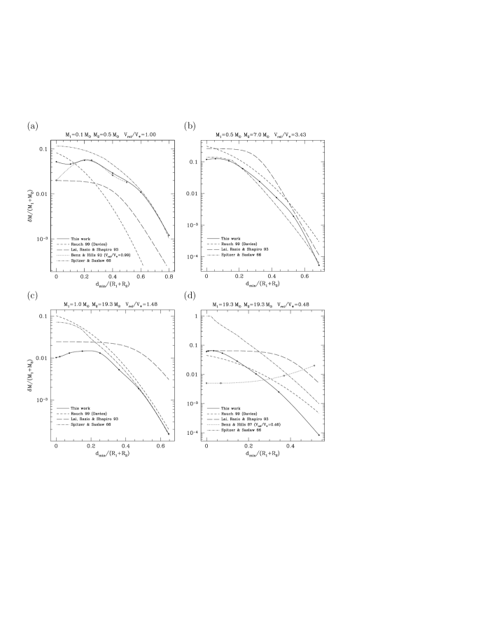
Figure 3.: Comparison of the fractional mass loss in some of our simulations with results and methods from the literature. In the case of Lai et al. (1993) and Rauch (1999), we compare to predictions from their fitting formulae. Benz & Hills (1987, 1992) do not publish such formulae so we compare directly to simulation results. To obtain the lines labeled “Spitzer & Saslaw (1966)” we applied the semi-analytical method invented by these authors to our stellar models.
These diagrams clearly illustrate that sensible comparisons can only be made with simulation results obtained with very similar initial conditions and stellar structures. For instance, our results are in good agreement with those of Benz & Hills for low mass stars (panel (a)) but completly at odds for $19.3\,M_{\odot}$ MS stars that are much more concentrated than their $n=1.5$ polytropes (panel (d)). Another example is panel (c) where we blindly push the published fitting formulae to a mass ratio much lower to the values for which they have been devised.

A zero-order description of the outcome of a stellar collision consists in the number of surviving stars. This is what we show in Fig. 4. Collisions with similar values of $q=M_{1}/M_{2}$ have been grouped on the same plot, regardless of the absolute values of the masses. Interestingly, in a initial conditions plane parameterized by “half-mass” quantities (see caption of figure), well defined borders appear that separate various outcome regimes. It also appears that, unless $V_{\mathrm{rel}}$ is very low, collisions that lead to coalescence (at low relative velocities) or complete disruptions (at high $V_{\mathrm{rel}}$) must be nearly head-on. By far the most likely outcome at velocities in excess of 100 km s^-1 is the preservation of both stars with only a small amount of mass loss. For small $M_{1}/M_{2}$ ratio, even head-on collisions do not necessarily result in mergers; the small star can fly through the large one without being stopped or destroyed. Such an effect, due to the high-mass star being of lower density than its small impacter was already proposed by Colgate (1967) to predict an upper mass limit to the process of run-away mergings. Whether this limiting mechanism really operates in dense stellar clusters has to be tested in dynamical simulations. It can be suppressed by mass segregation effects that drive most massive stars toward the center so that most important collisions take place between two high-mass stars.

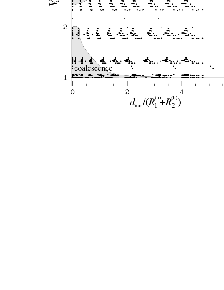
Figure 4.: Diagrams for the number of surviving stars in a selection of simulations. The left panel shows all simulations with $0.04\leq M_{1}/M_{2}\leq 0.09$ and the right panel all equal-mass encounters. Each dot stands for one SPH simulation. $R_{1}^{\mathrm{(h)}}$ and $R_{2}^{\mathrm{(h)}}$ are the radii that contain half the stellar mass of each star. $V_{\mathrm{cont}}$ is the relative velocity at “half-mass contact” (separation equal to $R_{1}^{\mathrm{(h)}}+R_{2}^{\mathrm{(h)}}$) and $V_{\ast}^{\mathrm{(h)}}=\sqrt{2G(M_{1}+M_{2})/(R_{1}^{\mathrm{(h)}}+R_{2}^{\mathrm{(h)}})}$. For almost all collisions in the white regions, there are two outgoing stars unbound to each other. Collisions in light gray regions results in a merger, a bound binary (prone to subsequent merging) or the disruption of one star. Finally, dark grey shading indicates complete destruction of both stars.

A more quantitative view on the results of 3 sets of collision simulations is given in panel (a) of Fig. 5 where we show the (interpolated) fractional mass loss in the $(d_{\mathrm{min}},V_{\mathrm{rel}})$ plane. Note how the “landscape” changes from one choice of $(M_{1},M_{2})$ to another one. This is another indication of the difficulty of finding a universal set of fitting formulae. The upper left white region of each diagram indicates $\delta M/M>85$ %. The small surface of this zone (in particular for unequal masses) means that such highly destructive events are unlikely. This is to be compared to the extent of the black regions for which the fractional mass loss is less than $10^{-4}$.

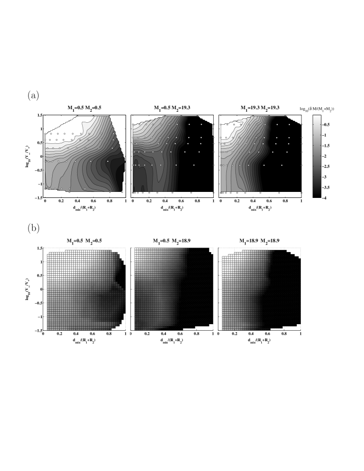
Figure 5.: Collisional fractional mass loss for three different $(M_{1},M_{2})$ pairs (values in $M_{\odot}$). (a) Simulation Data. White dots show the SPH simulations. Contours are a bicubic interpolation of the SPH results. (b) Interpolated grid.

3.3. Integration of collisions into the MC code

Being unable to distillate the results of our SPH simulation into any compact mathematical formulation without losing most of the information, we resorted to the following interpolation strategy. In the 4D initial parameter space, the simulations form a irregular grid of points. We compute a Delaunay triangulation of this set using the program Qhull (Barber, Dobkin, & Huhdanpaa 1996) which allows us to interpolate the results onto a regular 4D grid. Three slices in this grid are presented in Fig. 5(b). This table is used in MC simulations to determine – through a second interpolation – the outcome of collisions. Of course, extrapolation prescriptions have to be specified for events whose initial conditions fall outside the convex hull of the SPH simulation points. Most commonly, this happens when a collisionally produced star with mass outside the $0.1$–$74\,M_{\odot}$ range experience a further collision. In such cases, we try to re-scale both masses while preserving $M_{1}/M_{2}$ to get a “surrogate collision” lying in the domain covered by the SPH simulations. If $V_{\mathrm{rel}}$ is too low or too high, we increase or decrease it to enter the simulation domain. In many cases (for instance merging at low $V_{\mathrm{rel}}$ or complete destruction at high $V_{\mathrm{rel}}$), this method gives very sensible results. Encountyers with too high $d_{\mathrm{min}}$ are treated as purely Keplerian hyperbolic deflections with no mass loss.

4. Simulation of galactic nuclei evolution with stellar collisions

To illustrate the capacities of our “MC+SPH” approach and the role of collisions in the dynamics of dense galactic nuclei, we review some results from stellar dynamical simulations of simple nuclei models. The nominal model is a Plummer cluster with a scale radius of $R_{\mathrm{Plum}}=0.3$ pc that contains $5.09\times 10^{7}$ MS stars with a Salpeter mass spectrum: $dN/dM_{\ast}\propto M_{\ast}^{-2.35}$, $M_{\ast}\in[0.2,20]\,M_{\odot}$. In its center, we put a seed black hole ($M_{\mathrm{BH}}=10^{-6}M_{\mathrm{clst}}$) which is allowed to grow through accretion of stellar gas released in stellar collisions and tidal disruptions. Accretion is assumed to be complete and instantaneous. Stellar evolution is not simulated. The simulations were realized with 512 000 particles.

Fig. 6 shows snapshots of the density profile during the evolution of this model. When collisions are treated realistically, using our SPH grid, a steep central cusp with slope $\sim-1.75$ develops. This result is very similar to what is obtained when collisions are switched off and tidal disruptions are the only channel to consume stars (Bahcall & Wolf 1976, 1977). A milder slope of about $-1$ is obtained when collisions are assumed to result in complete stellar disruption. Even though we start with a model with very high central density, after a Hubble time, the mass density at 0.1–1 pc from the BH has reached a value similar to what is measured in the center of the Milky Way (Genzel et al. 1997). However, at that time, the BH’s mass in our model is about $10^{7}\,M_{\odot}$, nearly 4 times larger than Milky Way’s value. In Fig. 7, we compare the rates of mass accretion onto the central BH. When treated realistically, collisions dominate over tidal disruptions only during a short initial phase before massive stars segregate toward the center.

Figure 6.: Evolution of the cluster’s density profile for our “nominal model” (see text). (a) Collisions assumed to be completely disruptive. (b) Collisions modeled through SPH generated interpolation grid.

Figure 7.: Accretion rate on the central BH for three variations of the nominal model (see text). “Loss Cone” processes comprise tidal disruptions (dominant) and direct plunges through the BH’s horizon (very rare). (a) No collisions. (b) Disruptive collisions. (c) Realistic collisions (SPH).

We can not only explore the structure and evolution of the stellar cluster as a whole but also investigate some processes in more detail. For instance, it is possible to study the properties of individual collisions. In Fig. 8, we follow a selection of stars that experienced a large number of collisions. We report the distance to the center and the stellar mass before each collision. In a cluster without a central BH (panel (a)), the typical evolution of one of these frequently colliding stars is to sink toward the center while growing through a few mergers. In this simulation, the merging process is not allowed if the colliding star already has a mass beyond $\sim 60\,M_{\odot}$ but there is no doubt that it would otherwise lead to very massive stars. Of course such results may be significantly altered when stellar evolution is introduced. For instance, the star represented by the dotted line would not be able to wait during $\sim 7\times 10^{7}$ years between two successive mergers as the lifetime of a $20\,M_{\odot}$ star on the MS is only of order $10^{7}$ years. When a seed BH is present initially (panel (b)), it rapidly grows and leads to such an important increase in the stellar velocities near the center that mergers are totally quenched. Most collisions are then disruptive and the average stellar mass in the central regions actually decreases.

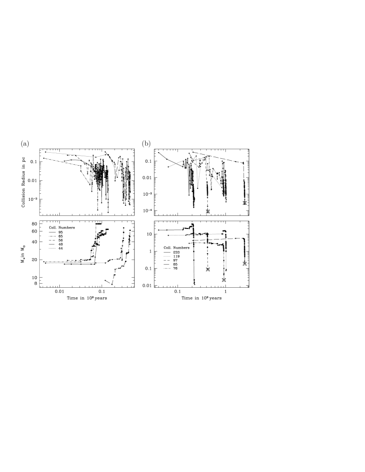
Figure 8.: Collisional histories for a few stars that experienced high numbers of collisions. We show the distance to the center (top) and the initial stellar mass (bottom) for each successive collision. A final star symbol indicates the “death” of the particle, either by complete disruption or by merging with a larger star. (a) No central BH. (b) Central BH with initial mass $M_{\mathrm{BH}}=10^{-6}M_{\mathrm{clst}}$. The labels are the total number of collisions for each particle.

5. Conclusions

When assumptions of spherical symmetry and dynamical equilibrium are reasonable, the Monte Carlo code for cluster dynamics appears as the method of choice to get detailed statistical predictions about the role and characteristics of collisions (and other physical processes) during the evolution of a stellar system. The use of SPH-based prescriptions to include collisions enables us to take the best advantage of the flexibility of the MC scheme in terms of realism.

Our models still lack other important and/or interesting physical aspects (stellar evolution, role of red giants and binaries,…). Other ingredients could be treated with more rigor. For instance, in the same spirit of our approach of stellar collisions, we could easily use the results of SPH simulations of tidal interactions between a star and the SBH (e.g. Fulbright 1996) to determine the outcome of these events. For the time being, we assume them to result in complete disruption of the star. More “realistic” prescriptions would not necessarily yield more reliable results, though, as the fraction of stripped stellar mass that is eventually accreted on the SBH is still a matter of debate (Ayal, Livio, & Piran 2000, and references therein). This illustrates the fact that many “improvements” could actually amount to adding more and more sources of uncertainty in the simulations. In such a context, it is all the more useful to dispose of a numerical tool flexible enough to allow changes in the treatment of various physical effects and fast enough to allow large sets of simulations to be conducted to test for the influence of these changes and the interplay between the many physical aspects of the problem.

Concerning the role of stellar collisions in the evolution of galactic nuclei, our present results may be considered disappointing. Indeed, even in cluster with quite extreme initial conditions (high stellar density), collisions do not leave any strong imprint on the overall structure of the stellar cluster. Neither do they feed the central BH more efficiently than tidal disruption or, presumably, stellar evolution. However, it must be stressed that collisions could have played a role of greater importance in the past if the present day nuclei have evolved from denser configurations. Further, more systematic sets of simulations will allow us to delineate the conditions leading to a collisional phase in the evolution of a cluster.

Furthermore, even if not efficient enough to rule the dynamics, collisions are interesting per se. More work is required to determinate the observational consequences of these events (creation of “exotic” stars, accretion of gas onto the central BH) but our code will stand as the central backbone for these future, more complete, studies.

Acknowledgments.

One of us (MF) wants to thank the organizers of this conference for partial financial support to attend it. This work has been supported in part by the Swiss National Science Foundation.

References

Alexander, T. & Kumar, P. 2000, ”Tidal Spin-up of Stars in Dense Stellar Cusps Around Black Holes”, preprint, astro-ph/0004240

Armitage, P. J., Zurek, W. H., & Davies, M. B. 1996, ApJ, 470, 237

Ayal, S., Livio, M., & Piran, T. 2000, ”Tidal Disruption of a Solar Type Star by a Super-Massive Black Hole”, preprint, astro-ph/0002499

Bahcall, J. N. & Wolf, R. A. 1976, ApJ, 209, 214

—. 1977, ApJ, 216, 883

Bailey, V. C. & Davies, M. B. 1999, MNRAS, 308, 257

Barber, C. B., Dobkin, D. P., & Huhdanpaa, H. T. 1996, ACM Transactions on Mathematical Software, 22, 469

Benz, W. 1990, in Numerical Modelling of Nonlinear Stellar Pulsations Problems and Prospects, 269

Benz, W. & Hills, J. G. 1987, ApJ, 323, 614

—. 1992, ApJ, 389, 546

Binney, J. & Tremaine, S. 1987, Galactic Dynamics (Princeton, NJ, Princeton University Press)

Charbonnel, C., Däppen, W., Schaerer, D., Bernasconi, P. A., Maeder, A., Meynet, G., & Mowlavi, N. 1999, A&AS, 135, 405

Coker, R. F. & Melia, F. 1997, ApJ, 488, L149

Colgate, S. A. 1967, ApJ, 150, 163

David, L. P., Durisen, R. H., & Cohn, H. N. 1987a, ApJ, 313, 556

—. 1987b, ApJ, 316, 505

Davies, M. B. 1996, in IAU Symp. 174: Dynamical Evolution of Star Clusters: Confrontation of Theory and Observations, Vol. 174, 243

Davies, M. B., Blackwell, R., Bailey, V. C., & Sigurdsson, S. 1998, MNRAS, 301, 745

Duncan, M. J. & Shapiro, S. L. 1983, ApJ, 268, 565

Freitag, M. 2000, ”Monte Carlo cluster simulations to determine the rate of compact star inspiraling to a central galactic black hole”, in preparation, to be published in the proceedings of the 3rd LISA Symposium

Freitag, M. & Benz, W. 2000a, ”A Comprehensive Set of Collision Simulations Between Main Sequence Stars”, in preparation

—. 2000b, ”A New Monte Carlo Code for Star Cluster Simulations”, in preparation

Fulbright, M. S. 1996, PhD thesis, University of Arizona

Genzel, R., Eckart, A., Ott, T., & Eisenhauer, F. 1997, MNRAS, 291, 219

Ghez, A. M., Morris, M., & Becklin, E. E. 1999, in ASP Conf. Ser. 182: Galaxy Dynamics - A Rutgers Symposium, 24

Giersz, M. 1998, MNRAS, 298, 1239

—. 2000, Monte Carlo simulations of star clusters - II. Tidally limited, multi-mass systems with stellar evolution, preprint, astro-ph/0009341

Hénon, M. 1973, in Lectures of the 3rd Advanced Course of the Swiss Society of Astronomy and Astrophysics (SSAA), 183

Hils, D. & Bender, P. L. 1995, ApJ, 445, L7

Ho, L. C. 1999, in Observational Evidence for the Black Holes in the Universe, 157

Joshi, K. J., Nave, C., & Rasio, F. 1999, ”Monte-Carlo Simulations of Globular Cluster Evolution - II. Mass Spectra, Stellar Evolution and Lifetimes in the Galaxy”, preprint, astro-ph/9912155

Joshi, K. J., Rasio, F. A., & Portegies Zwart, S. 2000, ApJ, 540, 969

Kim, S. S. & Lee, H. M. 1999, A&A, 347, 123

Kormendy, J. 2000, ”Supermassive Black Holes in Disk Galaxies”, preprint, astro-ph/0007401, to be published in “Galaxy Disks and Disk Galaxies”

Kormendy, J. & Richstone, D. 1995, ARA&A, 33, 581

Lai, D., Rasio, F. A., & Shapiro, S. L. 1993, ApJ, 412, 593

Lee, H. M. 1987, ApJ, 319, 801

Lightman, A. P. & Shapiro, S. L. 1977, ApJ, 211, 244

Lombardi, J. C., J., Rasio, F. A., & Shapiro, S. L. 1996, ApJ, 468, 797

Lombardi, J. C. J., Sills, A., Rasio, F. A., & Shapiro, S. L. 1999, Journal of Computational Physics, 152, 687

Makino, J. 2000, ”Direct Simulation of Dense Stellar Systems with GRAPE-6”, preprint, astro-ph/0007084

Maoz, E. 1998, ApJ, 494, 181

McMillan, S. L. W., Lightman, A. P., & Cohn, H. 1981, ApJ, 251, 436

Miralda-Escudé, J. & Gould, A. 2000, ”A Cluster of Black Holes at the Galactic Center”, preprint, astro-ph/0003269

Moran, J. M., Greenhill, L. J., & Herrnstein, J. R. 1999, Journal of Astrophysics and Astronomy, 20, 165

Murphy, B. W., Cohn, H. N., & Durisen, R. H. 1991, ApJ, 370, 60

Norman, C. & Scoville, N. 1988, ApJ, 332, 124

Portegies Zwart, S. F., Makino, J., McMillan, S. L. W., & Hut, P. 1999, A&A, 348, 117

Quinlan, G. D. & Shapiro, S. L. 1990, ApJ, 356, 483

Rasio, F. A. 2000, Monte Carlo Simulations of Globular Clusters Dynamics, preprint, astro-ph/0006205

Rauch, K. P. 1999, ApJ, 514, 725

Richstone, D., Ajhar, E. A., Bender, R., Bower, G., Dressler, A., Faber, S. M., Filippenko, A. V., Gebhardt, K., et al., 1998, Nature, 395, A14

Schaller, G., Schaerer, D., Meynet, G., & Maeder, A. 1992, A&AS, 96, 269

Seidl, F. G. P. & Cameron, A. G. W. 1972, Ap&SS, 15, 44

Shull, J. M. 1983, ApJ, 264, 446

Sigurdsson, S. & Rees, M. J. 1997, MNRAS, 284, 318

Sills, A., Faber, J. A., Lombardi, J. C., Rasio, F. A., & R., W. A. 2000, Evolution of Stellar Collision Products in Globular Clusters. II. Off-axis Collisions, preprint, astro-ph/0008254

Sills, A., Lombardi, J. C., Bailyn, C. D., Demarque, P., Rasio, F. A., & Shapiro, S. L. 1997, ApJ, 487, 290

Spitzer, L., J. & Saslaw, W. C. 1966, ApJ, 143, 400

Spitzer, L. 1987, ”Dynamical evolution of globular clusters” (Princeton, NJ, Princeton University Press, 1987, 191 p.)

Stodołkiewicz, J. S. 1982, Acta Astron., 32, 63

—. 1986, Acta Astron., 36, 19

Watters, W. A., Joshi, K. J., & Rasio, F. A. 2000, ApJ, 539, 331