Near-infrared Integral Field Spectroscopy and Mid-infrared Spectroscopy of the Starburst Galaxy M 82

Abstract

We present new infrared observations of the central regions of the starburst galaxy M 82. The observations consist of near-infrared integral field spectroscopy in the $H$- and $K$-band obtained with the MPE 3D instrument, and of $\rm\lambda=2.4-45~{}\mu m$ spectroscopy from the Short Wavelength Spectrometer (SWS) on board the Infrared Space Observatory. These measurements are used, together with data from the literature, to (1) re-examine the controversial issue of extinction, (2) determine the physical conditions of the interstellar medium (ISM) within the star-forming regions, and (3) characterize the composition of the stellar populations. Our results provide a set of constraints for detailed starburst modeling which we present in a companion paper.

We find that purely foreground extinction cannot reproduce the global relative intensities of H recombination lines from optical to radio wavelengths. A good fit is provided by a homogeneous mixture of dust and sources, and with a visual extinction of $A_{V}=52~{}{\rm mag}$. The SWS data provide evidence for deviations from commonly assumed extinction laws between 3$\,\mu$m and 10$\,\mu$m. The fine-structure lines of Ne, Ar, and S detected with SWS imply an electron density of $\approx~{}300~{}{\rm cm^{-3}}$, and abundance ratios Ne/H and Ar/H nearly solar and S/H about one-fourth solar. The excitation of the ionized gas indicates an average effective temperature for the OB stars of 37400 K, with little spatial variation across the starburst regions. We find that a random distribution of closely packed gas clouds and ionizing clusters, and an ionization parameter of $\approx 10^{-2.3}$ represent well the star-forming regions on spatial scales ranging from a few tens to a few hundreds of parsecs. From detailed population synthesis and the mass-to-$K$-light ratio, we conclude that the near-infrared continuum emission across the starburst regions is dominated by red supergiants with average effective temperatures ranging from 3600 K to 4500 K, and roughly solar metallicity. Our data rule out significant contributions from older, metal-rich giants in the central few tens of parsecs of M 82.

1 INTRODUCTION

M 82 is one of the nearest (3.3 Mpc; Freedman & Madore 1988; $\rm 1^{\prime\prime}=16~{}pc$), brightest, and best-studied starburst galaxies. It has long been considered as the archetype of this class of objects, and has often been used as test laboratory for starburst theories (see e.g. Telesco 1988 and Rieke et al.  1993 for reviews). The central 500 pc of M 82 harbours the most active starburst regions and has thus received particular attention in the past. Most of M 82’s infrared luminosity of $3\times 10^{10}~{}{\rm L_{\odot}}$ originates from this “starburst core,” which is severely obscured at optical and ultraviolet wavelengths.

The qualitative picture of M 82 features the following. A prominent nucleus, a stellar disk, and a kiloparsec-long stellar bar are revealed by near-infrared observations (e.g. Telesco et al. , 1991; McLeod et al. , 1993; Larkin et al. , 1994). The molecular gas resides mainly in a rotating ring or tightly wound spiral arms and in an inner spiral arm at radii of $\rm\approx 400~{}pc$ and $\rm\approx 125~{}pc$, respectively (e.g. Shen & Lo, 1995; Seaquist, Frayer, & Bell, 1998; Neininger et al. , 1998). The H II regions are concentrated in a smaller rotating ring-like structure of radius $\rm\approx 85~{}pc$, and along the stellar bar at larger radii (e.g. Larkin et al. , 1994; Achtermann & Lacy, 1995). HST observations have resolved over a hundred compact and luminous “super star clusters” across the central kiloparsec (O’Connell et al. , 1995; de Grijs, O’Connell, & Gallagher, 2000). An important series of young compact radio supernova remnants extends along the galactic plane over 600 pc (e.g. Kronberg, Biermann, & Schwab, 1985; Muxlow et al. , 1994; Pedlar et al. , 1999) and a bipolar outflow traces a starburst wind out to several kiloparsecs (e.g. Bregman, Schulman, & Tomisaka, 1995; Shopbell & Bland-Hawthorn, 1998; Lehnert, Heckman, & Weaver, 1999; Cappi et al. , 1999).

The triggering of starburst activity in M 82 is generally attributed to tidal interaction with its massive neighbour M 81 $\sim 10^{8}$ years ago or, alternatively, to the stellar bar which may itself have been induced by the interaction (e.g. Gottesman & Weliachew, 1977; Lo et al. , 1987; Yun, Ho, & Lo, 1993, 1994; Telesco et al. , 1991; Achtermann & Lacy, 1995). Beginning with the seminal paper by Rieke et al.  (1980), several authors have applied evolutionary synthesis modeling to understand the nature and evolution of starburst activity in M 82 (e.g. Bernlöhr, 1992; Rieke et al. , 1993; Doane & Mathews, 1993; Satyapal et al. , 1997). However, despite extensive studies, crucial issues remain open concerning in particular the composition of the stellar population and spatial variations thereof, the initial mass function of the stars formed in the starburst, and the spatial and temporal evolution of starburst activity.

In order to address the above issues quantitatively, we have obtained new observations of the central regions of M 82 consisting of near-infrared $H$- and $K$-band integral field spectroscopy with the Max-Planck-Institut für extraterrestrische Physik (MPE) 3D instrument (Weitzel et al. , 1996), and mid-infrared spectroscopy from the Short Wavelength Spectrometer (SWS; de Graauw et al. , 1996) on board the Infrared Space Observatory (ISO; Kessler et al. , 1996). The 3D data provide detailed information on small spatial scales from key features tracing the stellar populations and the interstellar medium (ISM) while the SWS data cover the entire $\rm\lambda=2.4-45~{}\mu m$ range containing a wealth of additional starburst signatures. The 3D and SWS data allow us to apply a variety of new and essential diagnostics which we use, together with results from the literature, to address several controversial issues and reveal additional aspects of M 82.

In this paper, we focus on characterizing the physical conditions of the ISM (gas density, abundances, extinction), the composition of the stellar populations (hot massive stars and cool evolved stars), and the relative distribution of the gas clouds and stellar clusters. In a companion paper (Förster Schreiber et al. 2000, in preparation; hereafter paper 2), we will apply recent starburst models to our results to constrain quantitatively the star formation parameters and the detailed starburst history in the central regions of M 82.

The paper is organized as follows. Section 2 describes the observations and data reduction procedure and section 3 presents the results. The physical conditions of the ISM are derived in section 4 together with the composition of the massive star population, while the composition of the cool evolved stellar population is investigated in section 5. Section 6 summarizes and discusses the results of our analysis.

2 OBSERVATIONS AND DATA REDUCTION

2.1 Near-infrared Data

We observed M 82 at near-infrared wavelengths using the MPE integral field spectrometer 3D (Weitzel et al. , 1996). A first data set was obtained at the 3.5 m telescope in Calar Alto, Spain, on 1995 January 13, 14, 16, and 21. The observations were completed at the 4.2 m William-Herschel-Telescope in La Palma, Canary Islands, on 1996 January 6. 3D slices the focal plane into 16 parallel “slits” which are imaged and dispersed in wavelength by a grism onto a 256$\times$256 HgCdTe NICMOS 3 array, providing simultaneously the entire $H$- or $K$-band spectrum of each spatial pixel. Nyquist-sampled spectra are achieved by dithering the spectral sampling by half a pixel on alternate data sets, which are interleaved in wavelength after the data reduction. For the M 82 observations, the instrument setup provided a pixel scale of $\rm 0.5^{\prime\prime}\,pixel^{-1}$ with a field of view of $8^{\prime\prime}\times 8^{\prime\prime}$, and a spectral resolution of $R\equiv\lambda/\Delta\lambda\approx 1015$ and $R\approx 830$ in the $H$- and $K$-band, respectively.

In order to sample representative starburst regions in M 82, we selected for the observations an area approximately $\rm 260~{}pc\times 160~{}pc$ (corresponding to $16^{\prime\prime}\times 10^{\prime\prime}$), nearly parallel to the plane of the galaxy. The regions mapped include the nucleus and extend to the west up to the inner edge of the molecular ring (see figure Near-infrared Integral Field Spectroscopy and Mid-infrared Spectroscopy of the Starburst Galaxy M 82 ). The 3D raster consists of four different fields, with adjacent fields overlapping by $\approx 3^{\prime\prime}$. Each field was observed in an object-sky-sky-object sequence, with the off-source frames taken on blank portions of the sky $2^{\prime}-4^{\prime}$ away in the north and south directions. The total on-source integration times per field and wavelength channel were $8-15$ and 10 minutes for the $H$- and $K$-band data, respectively. Typical single-frame exposures were $\rm 60-100~{}s$. For atmospheric calibration, we observed B-, late-F, or early-G dwarf stars each night, before and/or after M 82. The seeing varied from 1″ to 1.5″ during the observations. Table 1 summarizes the log of the observations.

We carried out the data reduction using the 3D data analysis package, within the GIPSY environment (van der Hulst et al. , 1992). We first performed correction for the non-linear signal response of the detector, dark current and background subtraction, spatial and spectral flat-fielding, wavelength calibration, rearrangement of the data in a three-dimensional cube, and bad pixel correction following standard procedures as described by Weitzel et al.  (1996). We reduced the reference stars data in the same manner. We then corrected the M 82 data cubes for atmospheric transmission by division with calibration spectra obtained as follows.

In the $K$-band, we first ratioed the stars spectra with a black-body curve of the appropriate temperature given their spectral type. We removed the intrinsic stellar features by division with the normalized spectrum of the G3 V star from the Kleinmann & Hall (1986) atlas, convolved to the resolution of 3D. This template has similar absorption line strengths as our F5 V and G0 V calibrators except for the Br$\gamma$ line, which we removed by linear interpolation. In the $H$-band, no appropriate template spectra were digitally available, so we constructed composite calibration spectra as follows. We generated synthetic transmission spectra between 1.55$\,\mu$m and 1.75$\,\mu$m at the proper zenithal distance using the program ATRAN (Lord, 1992). At the edges of the $H$-band, the transmission is very sensitive to the actual atmospheric conditions. Since our reference stars have no important features bluewards of 1.55$\,\mu$m and redwards of 1.75$\,\mu$m (within the range observed with 3D), we ratioed these portions of their spectrum with the appropriate blackbody curve and connected them to the synthetic spectra.

The residuals from intrinsic features of the reference stars are less than 1%. Those from telluric features do not exceed $3\%-4\%$ for most of the $H$- and $K$-band but amount up to 20% between 1.9$\,\mu$m and 2.0$\,\mu$m and at both edges of the $H$-band due to spatial and temporal variability of the atmospheric transmission. By fine-tuning the airmass for the calibration spectra with the help of ATRAN, we reduced the spurious features to less than 1% in the $K$-band and middle of the $H$-band, and less than 10% at the edges of the $H$-band.

For proper mosaicking, we smoothed the resulting data cubes with a two-dimensional gaussian profile to a common spatial resolution of 1.5″. The small scale structure is thus smeared out in the higher resolution fields but no important spatial features are lost. We combined the data cubes to produce the final mosaic, adjusting the mean broad-band flux in the overlapping areas to a common level. We performed absolute flux calibration based on the broad-band photometric measurements of Rieke et al.  (1980). We estimate the uncertainties on the absolute fluxes to be 15% in the $H$-band and 10% in the $K$-band. They include possible systematic errors in the relative spatial and spectral flux distribution which may occur in the background subtraction, in the correction for telluric absorption, and in the mosaicking (see also section 3.2).

2.2 Mid-infrared Data

We obtained the mid-infrared spectrum of M 82 with the SWS (de Graauw et al. , 1996) on board ISO (Kessler et al. , 1996) during revolution 116 on 1996 March 12. The grating scan mode AOT SWS01 was used to cover the entire SWS range from 2.4$\,\mu$m to 45$\,\mu$m. The slowest scan speed was selected to obtain the highest spectral resolution possible in this mode ($R\sim 500-1000$). In addition, individual lines were scanned with the grating line profile mode AOT SWS02 to get full resolving power ($R\sim 1000-2000$) and improved sensitivity for the key lines used in the data interpretation.

The SWS rectangular aperture was centered on the western mid-infrared emission peak (actual pointing at $\alpha_{1950}$: $\rm 09^{h}51^{m}42\fs 20$, $\delta_{1950}$: $+69^{\circ}55^{\prime}00\farcs 74$). The major axis of the aperture was oriented at a position angle of 64$\fdg$5, nearly parallel to the galactic plane of M 82. The aperture size varies from $14^{\prime\prime}\times 20^{\prime\prime}$ at short wavelengths to $20^{\prime\prime}\times 33^{\prime\prime}$ at long wavelengths. The SWS field of view thus includes the regions mapped with 3D, extending out to a maximum distance of about 350 pc from the nucleus (see figure Near-infrared Integral Field Spectroscopy and Mid-infrared Spectroscopy of the Starburst Galaxy M 82 ). The SWS full scan took in total $\rm 1^{h}50^{m}$. The on-source integration time for the individual line scans varied between 100 s for most lines and 600 s for the weakest lines.

We reduced the data with the SWS Interactive Analysis package (SIA), using special interactive extensions for glitch tail removal, dark subtraction, up-down correction, flat-fielding, and defringing. As the combined spectra of the 12 detectors of each SWS band are oversampled, we rebinned the final data to the proper instrumental resolution. We performed the calibration using the calibration tables as of 1998 February 15, equivalent to OLP version 7.0. The overall accuracy of the line and continuum fluxes is estimated to be $\approx 10\%-20\%$ (Schaeidt et al. , 1996; Salama et al. , 1997).

3 RESULTS

3.1 Near-infrared Spectra

We selected three individual regions within the 3D field of view for a detailed analysis: the nucleus, as well as two regions covering the Br$\gamma$ sources located approximately 10″ and 5″ southwest from the nucleus and which we designate as M82:Br1 and M82:Br2, respectively. For convenience, we will refer to the latter regions as “B1” and “B2” in the rest of this paper. B1 is close to the molecular ring and B2 coincides with the western mid-infrared emission peak. These three positions were chosen because they sample, along the galactic plane of M 82, representative regions with different spectral properties indicative of different stellar populations as described below.

We extracted the $H$- and $K$-band spectra of the individual regions from the 3D data cubes using synthetic apertures of $\rm 2.25^{\prime\prime}\times 2.25^{\prime\prime}$, corresponding to $\rm 35~{}pc\times 35~{}pc$. They are shown in figure Near-infrared Integral Field Spectroscopy and Mid-infrared Spectroscopy of the Starburst Galaxy M 82 together with those for the entire 3D field of view. All spectra exhibit the typical signatures of starburst activity, including H and He recombination lines tracing photoionized nebulae, ro-vibrational lines from warm $\rm H_{2}$, [Fe II] transition lines originating primarily in iron-enriched shocked material, and numerous atomic and molecular absorption features produced in the atmosphere of cool stars. However, the intensity of the features relative to the continuum varies with position. The emission lines become stronger along the sequence $\rm Nucleus\rightarrow B2\rightarrow B1$ while the stellar absorption features show the opposite trend.

Table 2 summarizes various continuum and line measurements obtained for the individual regions and for the 3D field of view. We computed the $H$- and $K$-band flux densities by averaging over the spectra of each region in the ranges $\rm\lambda=1.52-1.78~{}\mu m$ and $\rm\lambda=1.96-2.42~{}\mu m$, respectively. Throughout this paper, we will adopt the photometric system of Wamsteker (1981).

We measured the emission line fluxes by integrating over the line profile after subtracting a linear continuum fitted to adjacent line-free spectral regions. Due to the substantial continuum structure, these intervals were carefully selected by inspection of template spectra of K and M stars from existing stellar atlases (Kleinmann & Hall, 1986; Origlia, Moorwood, & Oliva, 1993; Dallier, Boisson, & Joly, 1996; Förster Schreiber, 2000) so that the linear interpolation adequately represented the underlying continuum. We tested the validity of this procedure by integrating the line fluxes after subtracting several template spectra of stars within $\rm\pm~{}3$ spectral classes of the representative type for each region (determined in section 5). We adopted the average fluxes, with uncertainties from the continuum subtraction corresponding to one standard deviation of the multiple measurements. At the spectral resolution of 3D, the Br11 and Br12 lines at 1.6807$\,\mu$m and 1.6407$\,\mu$m are blended with the [Fe II] lines at 1.6769$\,\mu$m and 1.6435$\,\mu$m, respectively. In these cases, we fitted double gaussian profiles to the features. The emission lines contribute at most 1.5% to the broad-band flux densities for all four regions.

We measured the equivalent widths (EWs) of the Si I absorption feature at 1.59$\,\mu$m, and of the $\rm{}^{12}CO$ (6,3) and $\rm{}^{12}CO$ (2,0) bandheads at 1.62$\,\mu$m and 2.29$\,\mu$m (denoted hereafter $W_{1.59}$, $W_{1.62}$, and $W_{2.29}$) according to the definitions and corrections for resolution effects given by Förster Schreiber (2000). Such corrections were necessary in order to compare the EWs for population synthesis purposes (section 5) with stellar data from existing libraries given for $R\sim 1600$ and $R\sim 2500$ in the $H$- and $K$-band, respectively. The Br14 emission line partially fills the Si I feature in all spectra. In order to remove this contamination, we scaled the profile of the Br13 line according to the intrinsic ratio $\rm Br14/Br13=0.80$ and subtracted it at the position of Br14. This ratio is for case B recombination (Hummer & Storey, 1987), assuming the electron density and temperature determined in section 4 ($n_{\rm e}=300~{}{\rm cm^{-3}}$ and $T_{\rm e}=5000~{}{\rm K}$). Differential extinction between these lines can be neglected because they are so close in wavelength.

3.2 Near-infrared Images

We obtained maps of the broad-band and line emission as well as of the EWs from the 3D data cubes by applying to each pixel the procedure described above for the spectra. Figure Near-infrared Integral Field Spectroscopy and Mid-infrared Spectroscopy of the Starburst Galaxy M 82 presents selected images and ratio maps.

The spatial distributions of the $H$- and $K$-band emission obtained with 3D agree well with maps in the literature (e.g. Dietz et al. , 1986; Telesco et al. , 1991; Larkin et al. , 1994; Satyapal et al. , 1995). The emission is generally centrally concentrated about the nucleus and small-scale structure is apparent, in particular the so-called “secondary peak” 8″ west from the nucleus. We assessed the accuracy of the flux calibration and mosaicking by comparing the $H$- and $K$-band flux densities measured at different positions between the 3D data and the large-scale images at 1″ resolution from Satyapal et al.  (1997), which were obtained with a single detector array. The relative flux densities between various regions agree typically to 15% in the $H$-band and 10% in the $K$-band. The differences may be due in part to the different spatial resolution of the data sets.

The Br$\gamma$ and He I 2.058$\,\mu$m line emission exhibit clumpy morphologies and follow each other very well. The ratio map, however, reveals spatial variations in the He I 2.058/Br$\gamma$ line ratio. The contrast between the distribution of the ionized gas and broad-band emission is well delineated by the logarithmic map of the ratio of $K$-band to Lyman continuum luminosities, $\log(L_{K}/L_{\rm Lyc})$. The Br$\gamma$ image obtained with 3D agrees well with previously published maps (Waller, Gurwell, & Tamura, 1992; Larkin et al. , 1994; Satyapal et al. , 1995). Table Near-infrared Integral Field Spectroscopy and Mid-infrared Spectroscopy of the Starburst Galaxy M 82 compares the Br$\gamma$ line flux integrated in circular apertures centered on the nucleus with measurements from the literature. The discrepancies between the various results are very large: up to a factor of 3.5. They are probably attributable to uncertainties in absolute calibration and continuum subtraction. In addition, positioning errors and differences in spatial resolution for linemaps could lead to appreciably different fluxes given the clumpy morphology of the emission. We have however no obvious explanation in the case of measurements at higher spectral resolution from well-registered linemaps, as for Larkin et al.  (1994) and Satyapal et al.  (1995). Both the spectral resolution and coverage as well as the quality of the 3D spectra allow a better continuum subtraction than in previous studies, supporting the accuracy of our Br$\gamma$ fluxes.

The $W_{2.29}$ and $W_{1.62}$ maps reveal very deep absorption features around the nucleus and the “secondary peak,” and progressively shallower features at B2 and B1. The $\log(W_{1.62}/W_{2.29})$ map is rather uniform but indicates an enhancement of $W_{1.62}$ relative to $W_{2.29}$ around B1. The $W_{2.29}$ image is consistent with the CO index map obtained at low spectral resolution by Satyapal et al.  (1997) within the regions observed with 3D.

The images demonstrate that the nucleus and B1 have the most extreme properties within the 3D field of view. The 3D maps and spectra indicate important spatial variations on relatively small scales in the composition of the stellar population, and support that the most recent star formation activity — as traced by the Br$\gamma$ emission for example — has taken place outside the nucleus, as noted previously (e.g. Telesco et al. , 1991; McLeod et al. , 1993; Satyapal et al. , 1997).

3.3 Mid-infrared Spectra

Figure Near-infrared Integral Field Spectroscopy and Mid-infrared Spectroscopy of the Starburst Galaxy M 82 shows the SWS full scan spectrum of M 82. Several H recombination lines from the Brackett, Pfund, and Humphreys series are detected as well as pure rotational lines from $\rm H_{2}$ and numerous fine-structure lines from various atoms mostly in low ionization stages. Broad emission features commonly attributed to polycyclic aromatic hydrocarbons (PAHs), a broad dip centered near 10$\,\mu$m, and a rising continuum at $\rm\lambda\gtrsim 10~{}\mu m$ likely due to very small dust grains are conspicuous (e.g. Gillett et al. , 1975; Willner et al. , 1977; Léger, d’Hendecourt, & Défourneau, 1989; Allamandola, Tielens, & Barker, 1989; Désert, Boulanger, & Puget, 1990; Roche et al. , 1991). According to Sturm et al.  (2000), the minimum around 10$\,\mu$m may not be due entirely to absorption by interstellar silicate grains as is usually assumed; the presence of strong flanking PAH emission complexes superposed over a weak continuum may contribute to the apparent dip. The higher signal-to-noise (S/N) ratio line scans are plotted in figure Near-infrared Integral Field Spectroscopy and Mid-infrared Spectroscopy of the Starburst Galaxy M 82 .

We measured the emission line fluxes from both the full scan SWS01 spectrum and the individual line scan SWS02 spectra. We fitted gaussian profiles to the features after subtraction of the continuum baseline obtained by fitting a line to adjacent line-free portions of the spectrum. Table 4 gives the line fluxes. In order to compare the data obtained with the different SWS apertures, we also scaled the fluxes of the H recombination and ionic fine-structure lines to the smallest $14^{\prime\prime}\times 20^{\prime\prime}$ aperture. We estimated the scaling factors from the [Ne II] 12.8$\,\mu$m map of Achtermann & Lacy (1995); they are 0.8 and 0.7 for the $14^{\prime\prime}\times 27^{\prime\prime}$ and $20^{\prime\prime}\times 33^{\prime\prime}$ apertures, respectively, with 10% uncertainty. The Br$\alpha$ 4.051$\,\mu$m, [Ar III] 8.99$\,\mu$m, and [S IV] 10.51$\,\mu$m maps obtained by these authors exhibit morphologies similar to that of the [Ne II] emission, justifying the use of the same scaling factors for all the hydrogen and fine-structure lines considered. No beam-size scaling was applied to the $\rm H_{2}$ lines because of the lack of information on the spatial distribution of the $\rm H_{2}$ emission. At the resolution of the SWS, the Br$\beta$ line (2.625$\,\mu$m) is blended with the $\rm H_{2}$ 1-0 $O$(2) line at 2.626$\,\mu$m. However, from the strength of the $\rm H_{2}$ 1-0 $Q$(3) at 2.423$\,\mu$m, we estimate that the $\rm H_{2}$ 1-0 $O$(2) line contributes at most 30% to the measured flux (Black & van Dishoeck, 1987; Sternberg & Dalgarno, 1989).

4 NEBULAR ANALYSIS OF M 82

In this section, we present our nebular analysis of M 82. We first derive the physical parameters critical for the interpretation of the nebular line emission: extinction, electron density, gas-phase abundances, and ionization parameter appropriate for the star-forming regions. We then use photoionization models to constrain the average effective temperature of the OB stars.

4.1 Interstellar Extinction

The issue of extinction towards the starburst regions of M 82 has long been controversial. In particular, extinctions in visual magnitudes $A_{V}$ ranging from a few to about 15 mag have been obtained under the assumption of a uniform foreground screen model or from optical and near-infrared diagnostics, while $A_{V}\approx 20-60~{}{\rm mag}$ have been inferred for a mixed model or from diagnostics at longer wavelengths (see e.g. McLeod et al.  1993, Satyapal et al.  1997, and references therein). Such differences may substantially affect the derived intrinsic properties (fluxes, luminosities). For instance, the correction factors at 2.2$\,\mu$m range from 1.6 to 4.1 assuming a uniform foreground dust screen with $A_{V}=5-15~{}{\rm mag}$, and from 2.2 to 5.7 assuming a mixed model with $A_{V}=20-60~{}{\rm mag}$ (see below for the computation of the correction factors). The discrepancies in extinction estimates can be understood in view of the large uncertainties in beam-size corrections involved in several studies, of those in the interpretation of some diagnostics (such as the broad dip around 10$\,\mu$m discussed above), of the spatially non-uniform extinction across the disk of M 82, and of the large optical depths preventing radiation at shorter wavelengths to escape from the most obscured regions (e.g. Puxley, 1991; Telesco et al. , 1991; McLeod et al. , 1993; Larkin et al. , 1994; Satyapal et al. , 1995, 1997; Sturm et al. , 2000).

4.1.1 Global Extinction towards the Ionized Gas

One major hindrance in previous studies has been the lack of data in the mid-infrared regime. ISO-SWS observations have now filled this gap, with a consistent set including several H recombination lines between $\rm 3\,\mu m$ and $\rm 10\,\mu m$. H recombination lines are excellent “standard candles” for extinction determinations because their intrinsic line emissivities are well determined theoretically. Moreover, the derived extinction parameters are fairly insensitive to the choice of electron density and temperature since the relative line emissivities vary slowly with these properties. For instance, the results from Hummer & Storey (1987) imply that the emissivities of the lines considered below change by 5% on average (18% at most) between $n_{\rm e}=10^{2}~{}{\rm cm^{-3}}$ and $\rm 10^{4}~{}cm^{-3}$, for $T_{\rm e}=5000~{}{\rm K}$. They vary by 20% on average (33% at most) between $T_{\rm e}=5000~{}{\rm K}$ and $\rm 10^{4}~{}K$, for $n_{\rm e}=10^{2}~{}{\rm cm^{-3}}$. The intrinsic Lyman continuum photon emission rates $Q^{0}_{\rm Lyc}$ derived from the dereddened line fluxes depend very weakly on $n_{\rm e}$, and vary only slightly with $T_{\rm e}$ since the total H recombination coefficient $\alpha_{\rm B}\propto T_{\rm e}^{-0.81}$. For the examples above, $Q^{0}_{\rm Lyc}$ increases on average by $\approx 5\%$ and 25%, respectively.

We combined our SWS data with H line measurements from the radio to the optical regimes, obtained mainly in large apertures (diameter $\gtrsim 20^{\prime\prime}$), and with appropriate beam-size corrections. Since the SWS and larger apertures include the most prominent emission regions (see the linemaps of McCarthy, Heckman, & van Breugel 1987, Satyapal et al.  1995, Achtermann & Lacy 1995, and Seaquist et al.  1996), the derived extinction should be representative for the bulk of ionized gas in M 82. A large wavelength coverage is essential for discriminating between various dust and sources geometries, since deviations from a simple uniform foreground screen model are perceptible only for diagnostics probing appreciably different optical depths.

In the range $\rm\lambda\sim 1-10~{}mm$, we used measurements for H26$\alpha$, H27$\alpha$, H41$\alpha$ (Seaquist et al. , 1996), H30$\alpha$ (Seaquist, Kerton, & Bell, 1994), H40$\alpha$ and H53$\alpha$ (Puxley et al. , 1989). The integrated fluxes for large apertures are consistent with predominantly optically thin, spontaneous emission in local thermodynamical equilibrium (LTE; see references above). We excluded data at centimeter wavelengths, which are potentially affected by stimulated emission and free-free absorption (e.g. Seaquist, Bell, & Bignell, 1985, 1996). At near-infrared wavelengths, we used the Brackett line fluxes measured with 3D. These were complemented with the Pa$\beta$ measurements from McLeod et al.  (1993) and Satyapal et al.  (1995), averaging the scaled fluxes together because of the large discrepancy between the two results (as for Br$\gamma$ discussed in section 3.2). Finally, at optical wavelengths, we used the H$\alpha$ measurement of McCarthy et al.  (1987). We obtained an additional estimate from the H$\alpha$ + [N II] $\lambda\lambda 6548,6584$ Å flux of Young, Kleinmann, & Allen (1988), assuming a uniform [N II]/H$\alpha$ ratio of 0.5 (McCarthy et al. , 1987).

We scaled the line fluxes to match the SWS $14^{\prime\prime}\times 20^{\prime\prime}$ beam in two steps. The fluxes were first scaled to a 30″–diameter aperture centered on the nucleus. The beam-size corrections for the millimeter lines were inferred from those derived by Seaquist et al.  (1994) between 19″, 21″, and 41″ apertures and the entire emission region, with an uncertainty of 15%. Those for the H$\alpha$ measurements were estimated from the map of McCarthy et al.  (1987), with 40% uncertainty. For Br$\gamma$ and Pa$\beta$, we applied a scaling $\propto\theta^{1.5}$ (where $\theta$ is the aperture diameter) derived from the Br$\gamma$ data of Satyapal et al.  (1995) in 3.8″, 8″, and 30″ apertures, with 10% uncertainty. Because of the weakness of the $H$-band Brackett lines within $\approx 5^{\prime\prime}$ of the nucleus, we used the fluxes integrated over the entire 3D map multiplied by the ratio of Br$\gamma$ fluxes scaled to a 30″ beam and measured in the 3D field of view. In the second step, a scaling factor $30^{\prime\prime}\rightarrow{\rm SWS}$ of 0.5 was applied, with 10% uncertainty, as derived by comparing various continuum and line fluxes from the SWS data with results reported in the literature, all of which presumably trace the same sources since they have similar spatial distributions; the references include Kleinmann & Low (1970), Rieke & Low (1972), Gillett et al.  (1975), Willner et al.  (1977), Houck et al.  (1984), Telesco, Dressel, & Wolstencroft (1993), and Achtermann & Lacy (1995). Table Near-infrared Integral Field Spectroscopy and Mid-infrared Spectroscopy of the Starburst Galaxy M 82 lists the observed and scaled line fluxes.

We derived the extinction by least-squares fitting to

$$\frac{F_{\lambda}}{F_{\rm ref}}=\left(\frac{j_{\lambda}}{j_{\rm ref}}\right)\left(\frac{X_{\lambda}}{X_{\rm ref}}\right),$$ (1)

where $F_{\lambda}/F_{\rm ref}$ are the observed line fluxes relative to that of a reference line, $j_{\lambda}/j_{\rm ref}$ are the intrinsic ratios of line emissivities, and $X_{\lambda}$ and $X_{\rm ref}$ are the attenuation factors due to extinction at the wavelengths of the lines considered. The SWS lines constituting the largest, self-consistent data set, we chose Br$\alpha$ as the reference line. We took the intrinsic line emissivities from Hummer & Storey (1987) for case B recombination with $n_{\rm e}=100~{}{\rm cm^{-3}}$ and $T_{\rm e}=5000~{}{\rm K}$, appropriate for M 82 as shown in section 4.2.1 . We adopted the extinction laws of Draine (1989) and Rieke & Lebofsky (1985) at infrared and optical wavelengths, respectively. At millimeter wavelengths, the extinction can be neglected.

We considered two representative model geometries. For a uniform foreground screen of dust (“UFS”), the attenuation is given by

$$X_{\lambda}^{\rm UFS}=\frac{I_{\lambda}}{I^{0}_{\lambda}}=e^{-\tau_{\lambda}},$$ (2)

where $I^{0}_{\lambda}$ and $I_{\lambda}$ are the intensities of the incident and emergent radiation, and $\tau_{\lambda}$ is the optical depth of the obscuring material. For a mixed model (“MIX”) consisting of a homogeneous mixture of dust and sources,

$$X_{\lambda}^{\rm MIX}=\frac{I_{\lambda}}{I^{0}_{\lambda}}=\frac{1-e^{-\tau_{\lambda}}}{\tau_{\lambda}}.$$ (3)

Here, $I^{0}_{\lambda}$ is the total intrinsic line intensity produced within the mixed medium, and $\tau_{\lambda}$ is the total optical depth of this medium. The extinction in magnitudes is related to the optical depth through $A_{\lambda}=1.086\,\tau_{\lambda}$.

The best fit for each model is achieved with a total visual extinction of $A_{V}^{\rm UFS}=4_{-4}^{+1.5}~{}{\rm mag}$ and $A_{V}^{\rm MIX}=43\pm 23~{}{\rm mag}$. We estimated the uncertainties on $A_{V}$ from the reduced chi-squared diagrams, with a $1\sigma$ error corresponding to a factor of $e^{1/2}$ from the minimum $\chi_{n}^{2}$. Table 6 compares the best-fit extinction-corrected line fluxes relative to Br$\alpha$ for each geometry (columns labeled “Draine”) with the intrinsic line ratios. Figure Near-infrared Integral Field Spectroscopy and Mid-infrared Spectroscopy of the Starburst Galaxy M 82 illustrates the results (plots labeled “Draine”), as the $Q^{0}_{\rm Lyc}$ derived from each of the extinction-corrected line fluxes assuming an average Lyman continuum photon energy of 15 eV. The average values of $Q^{0}_{\rm Lyc}$ are given in table 6.

Good extinction models are those for which equal values of $Q^{0}_{\rm Lyc}$ are inferred from each of the extinction-corrected line fluxes. Figure Near-infrared Integral Field Spectroscopy and Mid-infrared Spectroscopy of the Starburst Galaxy M 82 demonstrates that purely foreground extinction provides a much less satisfactory fit to the data over the entire wavelength range considered, as also shown by e.g. Puxley (1991) and McLeod et al.  (1993). The best fit for this geometry results in a minimum $\chi_{n}^{2}\approx 8$ compared to $\chi_{n}^{2}\approx 2$ for the mixed model. For the latter geometry, the extinction corrections are of 4.8 near 2$\,\mu$m and 1.6 near 5$\,\mu$m, with uncertainties of $\approx 50\%$ and $\approx 20\%$, respectively.

Increasing $n_{\rm e}$ to $\rm 10^{4}~{}cm^{-3}$ or $T_{\rm e}$ to $\rm 10^{4}~{}K$ results in larger $A_{V}$’s, but within the $1\sigma$ uncertainties for the nominal case. The implied values of $Q^{0}_{\rm Lyc}$ increase by about 15% and 50%, respectively. We also performed fits excluding the H$\alpha$ measurements, which may include a component from light escaping along the minor axis scattered by dust grains (e.g. O’Connell & Mangano, 1978; Notni, 1985). The H$\alpha$ flux could thus be overestimated relative to the data at longer wavelengths, since the scattering efficiency of interstellar dust grains generally decreases rapidly with increasing $\lambda$ (e.g. Emerson, 1988). The results for the mixed model are little affected, with $A_{V}^{\rm MIX}=44~{}{\rm mag}$ (a substantially larger $A_{V}^{\rm UFS}=9~{}{\rm mag}$ is obtained, as expected since the dust and sources are actually mixed). Fits excluding the millimeter lines yield $A_{V}^{\rm MIX}=18~{}{\rm mag}$, illustrating the importance of including unobscured lines.

4.1.2 The $\mathit{\lambda=3-10~{}\mu m}$ Extinction Law

Despite the good overall fit for the mixed model, figure Near-infrared Integral Field Spectroscopy and Mid-infrared Spectroscopy of the Starburst Galaxy M 82 indicates some deviations in the $\rm\lambda=3-10~{}\mu m$ region. The constraints imposed by the millimeter lines prevent reduction of these deviations by a change in absolute level of extinction. The extinction law assumed for these wavelengths may not be appropriate however. Indeed, until recently, the $\rm 3-10~{}\mu m$ extinction law was poorly determined because of the difficulties inherent to ground-based observations and because the properties of the template sources accessible so far in this range were not well-known. The SWS has now provided observations of numerous nebular H recombination lines between 3$\,\mu$m and 10$\,\mu$m in a variety of objects. These lines have been used to investigate the extinction law in the direction of the Galactic Center (Lutz, 1999). The “Galactic Center extinction law” (hereafter simply GC law) lacks the pronounced minimum in the $\rm 4-8~{}\mu m$ region expected for standard graphite-silicate dust mixtures which are usually assumed (e.g. Draine 1989 and references therein), suggesting additional contributors to the extinction.

The SWS line fluxes in M 82 are much better reproduced if the GC law is adopted. The best fits are obtained with $A_{V}^{\rm UFS}=4^{+2}_{-3}~{}{\rm mag}$ and $A_{V}^{\rm MIX}=52\pm 17~{}{\rm mag}$. The results are given in table 6 and figure Near-infrared Integral Field Spectroscopy and Mid-infrared Spectroscopy of the Starburst Galaxy M 82 (columns and plots labeled “GC”). The fit for the uniform foreground screen model is still much poorer than for the mixed geometry ($\chi_{n}^{2}\approx 8$ and $\approx 1$, respectively). The extinction corrections for the mixed model are 5.8 near 2$\,\mu$m and 2.6 near 5$\,\mu$m, with uncertainties of $\approx 30\%$ and 25%, respectively. Although the data do not allow the accurate determination of the extinction law in M 82, they provide evidence for deviations from the commonly used Draine law similar to those found towards the Galactic Center given by Lutz (1999).

4.1.3 Adopted Parameters

In view of the above analysis, we will adopt the mixed model with $A_{\it V}=52~{}{\rm mag}$ throughout this paper as representative of the global extinction towards the bulk of the ionized gas in M 82. The Lyman continuum photon emission rate for a 30″–diameter aperture is twice that for the SWS field of view (section 4.1.1), $Q^{0}_{\rm Lyc}=1.23\times 10^{54}~{}{\rm s^{-1}}$. Our results are consistent with the $Q^{0}_{\rm Lyc}$ inferred from the millimeter thermal free-free emission ($\rm\sim 10^{54}~{}s^{-1}$; e.g. Carlstrom & Kronberg 1991; Seaquist et al.  1996), and confirm the results of McLeod et al.  (1993) who found $A^{\rm MIX}_{V}=55~{}{\rm mag}$ and $Q^{0}_{\rm Lyc}=1.05\times 10^{54}~{}{\rm s^{-1}}$. We will also adopt the GC extinction law of Lutz (1999) between 3$\,\mu$m and 10$\,\mu$m, keeping the Draine (1989) law for the other relevant infrared ranges and the Rieke & Lebofsky (1985) law at optical wavelengths. Satyapal et al.  (1995) demonstrated the validity for M 82 of the Draine law at near-infrared wavelengths ($A_{\lambda}\propto\lambda^{-1.75}$), or of similar extinction laws (e.g. Landini et al.  1984, with $A_{\lambda}\propto\lambda^{-1.85}$).

4.1.4 Local Extinction towards the Ionized Gas

From the spatially resolved Brackett line emission obtained with 3D, we derived the extinction towards individual regions as described in section 4.1.1 using Br$\gamma$ as the reference line. The results for selected regions are reported in table 7, together with the $Q^{0}_{\rm Lyc}$ computed from the Br$\gamma$ fluxes (the most accurately measured line), corrected for $A_{V}^{\rm MIX}$. Due to the weakness of the $H$-band lines over significant areas, we could only generate a partial extinction map, from the 3D linemaps rebinned to $1^{\prime\prime}\times 1^{\prime\prime}$ pixels to increase the S/N ratio.

The variations in $A_{V}$ between individual regions and in our partial extinction map agree well with those seen in the extinction map of Satyapal et al.  (1995) obtained from Br$\gamma$ and Pa$\beta$ measurements. The lower $A_{V}^{\rm MIX}$ for the 3D field of view compared to the global extinction derived above probably reflects the optical depth limitations of the near-infrared diagnostics. For the same reasons, the derived $A_{V}^{\rm MIX}$ and $A_{V}^{\rm UFS}$ imply similar extinction corrections; for example, the differences are 35% or less near 2$\,\mu$m for the selected regions, and $\lesssim 20\%$ on the scale of the rebinned pixels over the valid regions. The uncertainties on the extinction corrections are typically $20\%-40\%$ for both models. As will be discussed in section 4.3, the ionized nebulae are likely mixed with the molecular gas and dust clouds even on scales of a few tens of parsecs. We will therefore adopt the results for the mixed model.

4.2 Physical Conditions of the ISM

4.2.1 Electron Temperature and Density

From the ratios of H recombination lines with the (thermal) continuum flux density in the millimeter regime, a $T_{\rm e}$ near 5000 K has been derived for the starburst core of M 82 (Puxley et al. , 1989; Carlstrom & Kronberg, 1991; Seaquist et al. , 1994, 1996). From the results of Seaquist et al.  (1996), based on maps of the H41$\alpha$ line emission and of the underlying continuum, we inferred that this temperature is appropriate on smaller spatial scales for most of the regions observed with 3D.

The SWS spectrum provides three density-sensitive ratios: [S III] 18.7$\,\mu$m/33.5$\,\mu$m, [Ne III] 15.6$\,\mu$m/36.0$\,\mu$m, and [Ar III] 8.99$\,\mu$m/21.8$\,\mu$m. All three are fairly insensitive to $T_{e}$ in the range $\rm 5000-20000~{}K$. The [S III] ratio is the most reliable one because both lines are amongst the strongest in the SWS spectrum. It is also the most sensitive at low $n_{\rm e}$ because the upper levels of the transitions have the lowest critical densities. For the $14^{\prime\prime}\times 20^{\prime\prime}$ SWS aperture, the dereddened suplhur, neon, and argon ratios are $0.71\pm 0.23$, $9.0\pm 4.2$, and $15.5\pm 9.3$, respectively. The uncertainties include those of the line flux measurements (from the relative flux calibration and continuum subtraction), and of the beam-size and extinction corrections. Comparison with results of computations of collisional excitation (e.g. Alexander et al. , 1999) shows that the measured ratios lie in the low-density limit, indicating $n_{\rm e}\sim 10-600~{}{\rm cm^{-3}}$.

Our result is similar to the average $n_{\rm e}$ in large apertures obtained previously by various authors using different infrared and radio diagnostics, and assuming a single-density model (Houck et al. , 1984; Duffy et al. , 1987; Seaquist et al. , 1985, 1996; Colbert et al. , 1999). We also considered the [O III] 52$\,\mu$m/88$\,\mu$m ratio, which is more sensitive to $n_{\rm e}$ at low densities. The ratio measured by Duffy et al.  (1987) in a 48″–diameter aperture, similar to the value for an 80″– aperture of Colbert et al.  (1999), indicates $n_{\rm e}\sim 50-500~{}{\rm cm^{-3}}$. We will adopt a value of $\rm 300~{}cm^{-3}$.

4.2.2 Gas-phase Abundances

We determined the gas-phase abundances of Ne, Ar, and S, three of the most abundant heavy elements in H II regions, using the lines detected with the SWS. These have critical densities for collisions with electrons at $T_{\rm e}=5000~{}{\rm K}$ in the range $\sim 10^{4}-10^{6}~{}{\rm cm^{-3}}$ so that collisional de-excitation can be neglected. Assuming a “one-layer” model with uniform density and temperature, the ionic abundances can be computed from

$$\frac{F_{\lambda({\rm X}^{+i})}}{F_{\lambda({\rm H}^{+})}}=\frac{n_{({\rm X}^{+i})}n_{\rm e}j_{\lambda({\rm X}^{+i})}}{n_{(\rm H^{+})}n_{\rm e}j_{\lambda({\rm H}^{+})}},$$ (4)

where $F_{\lambda({\rm X}^{+i})}$ and $F_{\lambda({\rm H}^{+})}$ are the fluxes of the ionic line of interest and of a reference H recombination line, $n_{({\rm X}^{+i})}$ and $n_{(\rm H^{+})}$ are the densities of ions $\rm X^{+i}$ and $\rm H^{+}$, and $j_{\lambda({\rm X}^{+i})}$ and $j_{\lambda({\rm H}^{+})}$ are the line emissivities. In H II regions, H is nearly completely ionized so that $n_{\rm H^{+}}\approx n_{\rm H}$. We computed the fine-structure line emissivities in the low-density limit using the effective collisional strengths from Johnson, Kingston, & Dufton (1986), Saraph & Tully (1994), Butler & Zeippen (1994), Pelan & Berrington (1995), and Galavís, Mendoza, & Zeippen (1995). We took Br$\alpha$ as reference H line, with its emissivity from Hummer & Storey (1987).

Table 8 gives the data and results. For ionizing stars with effective temperatures in the range $35000~{}{\rm K}-40000~{}{\rm K}$, as found in section 4.4 below, the Ne, Ar, and S are expected to be mostly in the ionization stages observed with SWS. The elemental abundances are thus well approximated by the sum of the ionic abundances determined here. The abundances are nearly solar or slightly above for Ne and Ar, and about one-fourth solar for S. Similar underabundances for S have been found in Galactic H II regions (e.g. Simpson et al. , 1995) and in some extragalactic starburst systems (e.g. Genzel et al. , 1998), and are attributed to depletion of S onto interstellar dust grains.

Most abundance determinations for M 82 in the literature indicate no large depletions or enhancements for most elements compared to the solar neighbourhood composition (e.g. Gaffney & Lester 1992; McLeod et al.  1993 and references therein; Achtermann & Lacy 1995; Lord et al.  1996). The exception is Si, for which Lord et al.  found a gas-phase abundance three times larger than in Galactic nebulae, and which they interpret as probably due to partial destruction of silicate grains by fast supernova-driven shocks.

4.3 Ionization Parameter

For the purpose of photoionization modeling, we represented H II regions as thin gas shells surrounding central, point-like stellar clusters (see top of figure Near-infrared Integral Field Spectroscopy and Mid-infrared Spectroscopy of the Starburst Galaxy M 82 ). In such “central cluster” models, the nebular conditions are specified by the distance $R$ between the ionizing cluster and the illuminated surface of the gas shell, the H number density $n_{\rm H}$, and the ionization parameter $U$ defined as

$$U\equiv\frac{Q_{\rm Lyc}}{4\pi R^{2}n_{\rm H}c}=\frac{\phi_{\rm Lyc}}{n_{\rm H}c},$$ (5)

where $Q_{\rm Lyc}$ is the production rate of Lyman continuum photons from the stars and $c$ is the speed of light. $U$ thus gives the number of Lyman continuum photons impinging at the surface of the nebula per H atom. Since H is nearly completely ionized in H II regions, and since He is not fully ionized in M 82 (section 4.4), we assumed $n_{\rm H}\approx n_{\rm e}$.

In such complex and distant systems as starburst galaxies, a large number of H II regions may coexist in a relatively small volume and may not be individually resolved by the observations. Thus, in constraining $U$ from the observed properties, the shell geometry may not be directly applicable. The spatial distribution of the gas relative to the sources is crucial in determining the Lyman continuum photon flux $\phi_{\rm Lyc}$ impinging on the gas, and in deriving the effective $U$ (hereafter $U_{\rm eff}$) to model appropriately the nebular emission in the framework of the idealized central cluster geometry. Due to the lack of information on small enough spatial scales, the ionization parameter is generally poorly determined in starburst galaxies. M 82 is one exception owing to its proximity. We have used our 3D and SWS data together with data from the literature to constrain the degree of ionization of the nebulae within the starburst regions. Appendix A gives the details of our derivation; in the following, we restrict ourselves to outlining the main results.

The ISM properties within the starburst regions of M 82 (e.g. Lord et al. , 1996) suggest it can be represented by a collection of clouds with, on average, a molecular core with radius $\rm\approx 0.5~{}pc$ shielded by a thin neutral atomic layer, and an ionized layer extending out to $\rm\approx 1~{}pc$. These clouds have a mean separation of $\rm\approx 2-7~{}pc$. High resolution optical and near-infrared imaging reveals large numbers of young, luminous clusters throughout the starburst core (e.g. O’Connell et al. , 1995; Satyapal et al. , 1997). Assuming the OB stars reside in such clusters and adopting a plausible cluster luminosity function consistent with the properties of the optically-selected population, the intrinsic Lyman continuum photon emission rates imply an average cluster separation of $\rm 2-9~{}pc$.

The similar cloud-cloud and cluster-cluster mean separations suggests that the clouds and clusters are well-mixed and uniformly distributed throughout the regions of interest, as illustrated at the bottom of figure Near-infrared Integral Field Spectroscopy and Mid-infrared Spectroscopy of the Starburst Galaxy M 82 . For such a random distribution model, the flux of Lyman continuum photons impinging on the nebulae is reduced compared to the central cluster geometry due to the increase in surface area of the gas exposed to the radiation field. From the analysis of selected regions in appendix A, we determine $\log U_{\rm eff}\approx-2.3~{}{\rm dex}$ and conclude that it is representative of the local nebular conditions throughout all of the star-forming regions in the central 500 pc of M 82. We also show that $U_{\rm eff}$ can be expressed in terms of the ratio of intrinsic Lyman continuum photon emission rate and of the molecular gas mass, with $U_{\rm eff}\propto Q_{\rm Lyc}/M_{\rm H_{2}}$ and the proportionality factor depending only on the gas cloud properties (see equation [A4]). Since the cloud properties are similar throughout the starburst core of M 82, the comparable values of $\log U_{\rm eff}$ are interpreted as resulting from comparable star formation efficiencies as measured by $Q_{\rm Lyc}/M_{\rm H_{2}}$.

4.4 Young Stellar Populations

The SWS and 3D data provide several diagnostics sensitive to the shape of the ionizing radiation spectrum, dominated by OB stars in M 82. These include ratios of mid-infrared atomic fine-structure lines and of near-infrared He to H recombination lines, which probe the $\rm 13~{}eV-41~{}eV$ energy range. The contribution from shock-ionized material to the line emission considered below is not likely to be important in M 82 (McLeod et al. , 1993; Lutz et al. , 1998). In the following, we will assume that the lines originate entirely in gas photoionized by the OB stars. Table 9 summarizes the data and results.

4.4.1 Mid-infrared Fine-structure Line Ratios

Amongst the diagnostic line ratios available from the SWS data set, we considered [Ne III] 15.6$\,\mu$m/[Ne II] 12.8$\,\mu$m, [Ar III] 8.99$\,\mu$m/[Ar II] 6.99$\,\mu$m, and [S IV] 10.5$\,\mu$m/[S III] 18.7$\,\mu$m to avoid complications due to the uncertainties of the elemental abundances.

We modeled the variations of the line ratios with effective temperature of the stars ($T_{\rm eff}^{\rm OB}$) using the photoionization code CLOUDY version C90.05 (Ferland, 1996) and the stellar atmosphere models for solar-metallicity main-sequence stars of Pauldrach et al.  (1998). We adopted the nebular parameters derived in the previous subsections: solar gas-phase abundances, $n_{\rm e}=300~{}{\rm cm^{-3}}$, and an effective $\log U=-2.3~{}{\rm dex}$. With this value for the ionization parameter, equation (5) implies a corresponding $R$ of several tens to several hundreds of parsecs, depending on the region. Since photoionization models are little sensitive to variations in $R$ above $\rm\sim 10~{}pc$, we adopted a fixed $R=25~{}{\rm pc}$. We neglected the effects of dust grains possibly present within the nebulae. Dust grains mixed with the ionized gas are not expected to affect significantly the ionization equilibrium of H II regions because the variations of the dust absorption cross-section with wavelength resembles closely that of H, peaking near 17 eV (e.g. Mathis, 1986). Mathis further argues that this conclusion is not altered for dust properties and gas-to-dust ratios characteristic of the Galactic and Magellanic Clouds diffuse ISM or of denser H II regions.

Figure Near-infrared Integral Field Spectroscopy and Mid-infrared Spectroscopy of the Starburst Galaxy M 82 shows the theoretical predictions and the measured ratios, corrected for extinction and beam-size differences when appropriate. The effects of variations of $n_{\rm e}$ and $\log U$, or of adopting a gas and dust composition typical of the Orion nebula are also indicated. The most sensitive parameter affecting the line ratios is the ionization parameter. However, varying $\log U$ in the plausible range from $-2$ to $-2.5~{}{\rm dex}$ (see appendix A) implies relatively small differences in $T_{\rm eff}^{\rm OB}$: $\leq\pm 1000~{}{\rm K}$ for the neon and argon ratios, and $\rm-2000~{}K$ or $+4000~{}{\rm K}$ for the sulphur ratio. Given the uncertainties of the data (line measurements, extinction and aperture corrections) as well as of the models (e.g. nebular parameters, stellar atmospheres, atomic data), the agreement between the results from the three diagnostic ratios is satisfactory. Our high quality and consistent data set confirms results obtained in the past from various infrared and millimeter lines, which ranged from 30000 K to 37000 K (Gillett et al. , 1975; Willner et al. , 1977; Puxley et al. , 1989; McLeod et al. , 1993; Achtermann & Lacy, 1995; Colbert et al. , 1999).

4.4.2 Near-infrared He to H Recombination Line Ratios

The strongest recombination lines from singly-ionized He detected in the 3D spectra correspond to the $2\,^{1}S-2\,^{1}P$ triplet transition at 2.058$\,\mu$m and the $3\,^{3}P-4\,^{3}D$ singlet transition at 1.701$\,\mu$m . Together with the nearby Br$\gamma$ and Br10 lines, respectively, they provide $T_{\rm eff}^{\rm OB}$ diagnostics sensitive in the range $\rm\lesssim 55000~{}K$ and very little affected by extinction. The low-excitation SWS spectrum and the non-detection of He II lines in the 3D data (for example at 2.189$\,\mu$m) rule out the presence of important populations of Wolf-Rayet stars or other sources that are hot enough to doubly ionize He, which would complicate the interpretation of the ratios.

The He I 2.058/Br$\gamma$ line ratio has been commonly used to estimate $T_{\rm eff}^{\rm OB}$ in near-infrared studies of starburst galaxies and Galactic H II regions (e.g. Doyon, Puxley, & Joseph, 1992; Doherty et al. , 1994, 1995). However, due to sensitivity to local physical conditions and to degeneracy in $T_{\rm eff}^{\rm OB}$ through resonance and collisional effects (e.g. Robbins, 1968; Clegg, 1987; Shields, 1993), this ratio alone is not sufficient for constraining $T_{\rm eff}^{\rm OB}$. On the other hand, the 1.701$\,\mu$m line originates from a higher quantum state in the $n\,^{3}P-n^{\prime}\,{}^{3}D$ series and is essentially unaffected by self-absorption and collisional effects but the He I 1.701/Br10 ratio saturates above $T_{\rm eff}^{\rm OB}\approx 40000~{}{\rm K}$ (see references above). Therefore, the combination of the He I 2.058/Br$\gamma$ and He I 1.701/Br10 ratios allows one to discriminate between the high- and low-$T_{\rm eff}^{\rm OB}$ regimes (see e.g. Vanzi et al.  1996 and Doherty et al.  1995 for earlier applications).

We modeled the He to H line ratios using CLOUDY and the same model atmospheres and nebular parameters as for the mid-infrared line ratios. CLOUDY computes the 2.058$\,\mu$m line but not the 1.701$\,\mu$m line which we derived indirectly as explained below. While models of He I 2.058/Br$\gamma$ presented by various authors in the past generally agree very well in the range $T_{\rm eff}^{\rm OB}\leq 40000~{}{\rm K}$, the results at higher $T_{\rm eff}^{\rm OB}$ vary importantly (Doyon et al. , 1992; Shields, 1993; Doherty et al. , 1994, 1995; Lançon & Rocca-Volmerange, 1994). In this regime, the ratio is particularly sensitive to the treatment of the He I Ly$\alpha$ opacity which is one of the major sources of uncertainties in theoretical predictions. Ferland (1999) discusses the revised treatment implemented in the CLOUDY version we have used.

For He I 1.701$\,\mu$m, we used the He I 4471 Å flux predicted by CLOUDY. Both lines originate from the $4\,^{3}D$ level and their fluxes are proportional to each other since triplet transitions from high $n\,^{3}D$ levels are essentially unaffected by collisional effects or scattering from the metastable $2\,^{3}S$ level. We scaled the resulting He I 4471 Å/Br10 curve so that its saturation value for full He ionization equals that for He I 1.701/Br10 given by Vanzi et al.  (1996). While $n_{\rm e}$ is fixed in running CLOUDY, $T_{\rm e}$ varies for each $T_{\rm eff}^{\rm OB}$; we thus interpolated the relationship of Vanzi et al.  in $T_{\rm e}$ as appropriate. Since collisions are unimportant for both He lines involved here, we used this relationship up to $n_{\rm e}=10^{3}~{}{\rm cm^{-3}}$.

The ratios measured for selected regions are plotted against the model predictions in figure Near-infrared Integral Field Spectroscopy and Mid-infrared Spectroscopy of the Starburst Galaxy M 82 . The He I 1.701/Br10 ratio clearly rules out the high-$T_{\rm eff}^{\rm OB}$ solutions from the He I 2.058/Br$\gamma$ ratio. For the temperatures near 36000 K inferred, He I 2.058/Br$\gamma$ and He I 1.701/Br10 are little affected by variations in $n_{\rm e}$ or $\log U$ within plausible ranges for M 82, or by modest changes in the gas and dust composition. Again, in view of the uncertainties of the data and models (in particular the continuum subtraction for the $H$-band lines), the $T_{\rm eff}^{\rm OB}$’s inferred for each region from both ratios agree satisfactorily.

The variations in our He I 2.058/Br$\gamma$ map (figure Near-infrared Integral Field Spectroscopy and Mid-infrared Spectroscopy of the Starburst Galaxy M 82 ) support a general though small increase in $T_{\rm eff}^{\rm OB}$ from the nucleus to larger projected radii along the galactic plane of M 82 to the west. Such radial variations have been suggested by Satyapal et al.  (1995) from the ratio of Br$\gamma$ to 3.29$\,\mu$m PAH feature emission. McLeod et al.  (1993) also suggested such a trend from the lower temperatures derived from mid-infrared diagnostics compared to those inferred from optical diagnostics assuming the former trace the innermost stellar population while the latter, foreground and thus outermost clusters. On the other hand, Achtermann & Lacy (1995) concluded that $T_{\rm eff}^{\rm OB}$ is roughly constant across the starburst core from the lack of clear spatial variations in the excitation state from their Br$\alpha$, [Ne II] 12.8$\,\mu$m, [Ar III] 8.99$\,\mu$m, and [S IV] 10.5$\,\mu$m maps.

We constrained quantitatively the spatial variations in $T_{\rm eff}^{\rm OB}$ across the 3D field of view from our He I 2.058$\,\mu$m and Br$\gamma$ linemaps, rebinned to $1^{\prime\prime}\times 1^{\prime\prime}$ pixels. We neglected extinction effects, but this introduces errors $\lesssim 5\%$ in the ratios. The resulting $T_{\rm eff}^{\rm OB}$’s vary from 33200 K to 37500 K, with an average of 35700 K and a relatively small dispersion of $1\sigma=650~{}{\rm K}$. The 3D data indicate therefore a roughly constant $T_{\rm eff}^{\rm OB}$ for the hot massive stars across the regions observed, with only a marginal gradient with projected radius.

4.4.3 Additional Remarks

From our data sets, the neon ratio is probably the most reliable indicator for the absolute $T_{\rm eff}^{\rm OB}$. Both lines involved are strong in M 82 and, among the three mid-infrared line pairs, their proximity in wavelength minimizes most extinction effects and they were observed through the same aperture. It is also the most sensitive of all our diagnostics, probing the largest range in ionizing energy (between 22 eV and 41 eV). In addition, the inferred $T_{\rm eff}^{\rm OB}$ is little affected by the uncertainties on the physical conditions within the nebulae. The He I 2.058/Br$\gamma$ and He I 1.701/Br10 are potentially less reliable indicators for the absolute $T_{\rm eff}^{\rm OB}$ because directly sensitive to the He abundance. On the other hand, for the ranges observed in M 82, these ratios are little affected by modeling uncertainties and are thus robust diagnostics for the relative variations in $T_{\rm eff}^{\rm OB}$ (assuming negligible gradients in He abundance). Since the smaller SWS aperture and the 3D field of view cover the same most prominent sources, the nebular line emission from both data sets traces essentially the same stellar populations. In the rest of this work, we will adopt the result from the neon ratio (37400 K) for the 3D and SWS fields of view and will apply a correction of $\rm+1400~{}K$ to the temperatures inferred from He I 2.058/Br$\gamma$, corresponding to the difference in $T_{\rm eff}^{\rm OB}$ obtained from the neon ratio and that for the 3D field of view.

From the temperature scale of Vacca, Garmany, & Shull (1996), the inferred $T_{\rm eff}^{\rm OB}$’s within the 3D and SWS fields of view correspond to O8.5 V stars, with $Q^{\rm O8.5\,V}_{\rm Lyc}=10^{48.72}~{}{\rm s^{-1}}$. Given the roughly constant nebular excitation and the SWS aperture including half of the integrated emission in a 30″–diameter region centered on the nucleus of M 82, this spectral type is probably representative of the dominant OB stars for the starburst core as well. The number of equivalent O8.5 V stars required to produce the intrinsic Lyman continuum luminosity in various regions is given in table 9.

5 STELLAR POPULATION SYNTHESIS OF M 82

In this section, we apply population synthesis to our 3D data. We constrain the spectral type and luminosity class of the evolved stars, and investigate their metallicity. We also constrain the contribution from additional continuum sources (hot dust, OB stars, nebular free-free and free-bound processes) as well as the extinction towards the evolved stars. All results are reported in table 10.

5.1 Analysis of Selected Absorption Features

5.1.1 The Giants-supergiants Controversy

The nature of the evolved stellar population in M 82 has long been debated. Various diagnostics have been used in the past, including the near-infrared broad-band colours, the $CO_{\rm ph}$ and $H_{2}O_{\rm ph}$ photometric indices measuring the depth of the CO bandheads longwards of 2.3$\,\mu$m and of the $\rm H_{2}O$ absorption feature at 1.9$\,\mu$m, spectral synthesis in the range $\rm 2.18~{}\mu m-2.28~{}\mu m$, and measurements of the ratio of stellar mass to intrinsic $K$-band luminosity $M^{\star}/L_{K}$ (Walker, Lebofsky, & Rieke, 1988; Lester et al. , 1990; Gaffney & Lester, 1992; Gaffney, Lester, & Telesco, 1993; McLeod et al. , 1993; Lançon, Rocca-Volmerange, & Thuan, 1996). Evolutionary synthesis models have also been applied to obtain indirect constraints (Rieke et al. , 1980, 1993; Satyapal et al. , 1997).

However, no consensus has been reached yet, in particular concerning the nucleus: some of the above studies indicate the presence of young supergiants while others provide evidence for old, metal-rich giants as dominant sources of the near-infrared continuum emission. Possible causes for these discrepancies include positioning uncertainties and dependence on aperture size due to important spatial variations in the indicators, difficulties inherent to measurements of $H_{2}O_{\rm ph}$ (in a range of poor atmospheric transmission), and the weakness of several absorption features. More importantly, the diagnostics used so far exhibit degeneracy in temperature and luminosity, and are affected by extinction and featureless continuum emission.

The 3D data allow us to apply alternative diagnostic tools. The CO bandheads at 2.29$\,\mu$m and 1.62$\,\mu$m together with the Si I feature at 1.59$\,\mu$m are particularly useful in stellar population studies from moderate-resolution near-infrared spectra (Origlia et al. , 1993; Oliva et al. , 1995; Förster Schreiber, 2000). They suffer much less from measurements uncertainties and provide sensitive indicators for the effective temperature and luminosity class of cool stars. Moreover, their EWs ($W_{2.29}$, $W_{1.62}$, and $W_{1.59}$) are independent of extinction and provide a means of constraining the contribution, or “dilution,” from featureless continuum emission sources without requiring any assumptions on their nature and physical properties.

In the following analysis, we neglect possible contributions from thermally-pulsing AGB stars (such as Mira variables and N-type carbon stars) since none of their extreme, characteristic features (e.g. Johnson & Méndez, 1970; Lançon et al. , 1999) are seen in the 3D spectra. Moreover, evolutionary synthesis models show that these stars never produce more than $10\%-40\%$ of the integrated near-infrared light of stellar clusters of any age (e.g. Bruzual & Charlot 1993; paper 2).

5.1.2 Selected Regions

We analyzed the EWs using the diagnostic diagrams proposed by Origlia et al.  (1993) and Oliva et al.  (1995). These are shown in figures Near-infrared Integral Field Spectroscopy and Mid-infrared Spectroscopy of the Starburst Galaxy M 82 and Near-infrared Integral Field Spectroscopy and Mid-infrared Spectroscopy of the Starburst Galaxy M 82 , where the stellar data has been obtained from existing relevant libraries (as compiled by Förster Schreiber 2000). The horizontal bars indicate the measurements for selected regions in M 82; those for the 3D field of view are omitted for clarity, but are very close to those for B2. Figure Near-infrared Integral Field Spectroscopy and Mid-infrared Spectroscopy of the Starburst Galaxy M 82 gives the effective temperature ($T_{\rm eff}$) and luminosity class implied by the EWs. Figure Near-infrared Integral Field Spectroscopy and Mid-infrared Spectroscopy of the Starburst Galaxy M 82 allows the determination of the amount of dilution near 1.6$\,\mu$m ($D_{1.6}$) from the vertical displacement relative to the locus of stars in the $W_{1.62}$ versus $\log(W_{1.62}/W_{1.59})$ diagram, and near 2.3$\,\mu$m ($D_{2.3}$) from the horizontal displacement in the $W_{1.62}$ versus $\log(W_{1.62}/W_{2.29})$ diagram once $W_{1.62}$ is corrected for dilution. As shown by Oliva et al.  (1995), undiluted composite stellar populations fall on the distributions defined by the stars in these plots.

For the central 35 pc at the nucleus of M 82, both $W_{1.62}$ and $\log(W_{1.62}/W_{1.59})$ indicate an average effective temperature in the range $\rm 3600-4100~{}K$, implying negligible dilution around 1.6$\,\mu$m. The $W_{2.29}$ is characteristic of either giants with $T_{\rm eff}=3200-3600~{}{\rm K}$ or supergiants with $T_{\rm eff}=3600-4200~{}{\rm K}$. Therefore, the EWs can only be reconciled for a population of supergiants and negligible dilution in both $H$- and $K$-band. Using the temperature calibration of Schmidt-Kaler (1982), the corresponding average spectral type is K5 I. For the other selected regions, degeneracy in luminosity class and dilution complicates the interpretation of the EWs. In all cases, $W_{1.62}$ and $\log(W_{1.62}/W_{1.59})$ imply negligible dilution near 1.6$\,\mu$m. For B1, the data indicate dominant K3 III stars and $D_{2.3}\approx 10\%$ or K2 I stars and $D_{2.3}\approx 10\%-40\%$. For B2 and the 3D field of view, the EWs are more consistent with K3-K4 supergiants and small amounts of dilution near 2.3$\,\mu$m, but undiluted emission from K4 giants cannot be completely ruled out. However, we favoured the supergiants solutions on the basis of the ratio of stellar mass to intrinsic $K$-band luminosity $M^{\star}/L_{K}$, as explained below.

5.1.3 Spatially Detailed Analysis

We applied a similar analysis to all the regions observed with 3D, using maps of the $W_{1.59}$, $W_{1.62}$, and $W_{2.29}$ generated from the data cubes rebinned to $1^{\prime\prime}\times 1^{\prime\prime}$ pixels. We corrected the $W_{1.59}$ map for contamination by the Br14 emission line as described in section 3.1. The resulting spectroscopic indices for all pixels are plotted in the diagnostic diagrams of figure Near-infrared Integral Field Spectroscopy and Mid-infrared Spectroscopy of the Starburst Galaxy M 82 .

Together with the EW maps from figure Near-infrared Integral Field Spectroscopy and Mid-infrared Spectroscopy of the Starburst Galaxy M 82 , figure Near-infrared Integral Field Spectroscopy and Mid-infrared Spectroscopy of the Starburst Galaxy M 82 reveals variations in the intrinsic composition of the evolved stellar population on small spatial scales, little dilution around 1.6$\,\mu$m, and variable dilution around 2.3$\,\mu$m. The inferred $T_{\rm eff}$’s range from 4500 K down to 3600 K, corresponding to spectral types G9 to M0 for supergiants. The average is 4000 K with dispersion of $1\sigma=200~{}{\rm K}$, equivalent to K4 $\pm$ two spectral sub-classes assuming supergiants. Several regions lie on the locus of supergiants in the $W_{1.62}$ versus $\log(W_{1.62}/W_{2.29})$ diagram; they also coincide with the brightest $K$-band sources. Others are characterized by too small $W_{2.29}$ relative to $W_{1.62}$ compared to normal evolved stars, implying significant dilution near 2.3$\,\mu$m up to $\approx 50\%$ assuming an intrinsic population of supergiants ($\approx 20\%$ for giants). Because dilution in the $H$-band is negligible, the $W_{1.62}$ map constitutes essentially a $T_{\rm eff}$ map for the evolved stars, showing spatial variations that are more complex than simple radial gradients. The coolest populations are found around the nucleus and along a ridge extending up to the secondary $K$-band peak ($\approx 8^{\prime\prime}$ to the west). Just south from this ridge, the $T_{\rm eff}$ increases progressively along the Nucleus $\rightarrow$ B2 $\rightarrow$ B1 sequence.

For most individual regions, the $\log(W_{1.62}/W_{2.29})$ does not allow the discrimination between giants and supergiants due to degeneracy in luminosity class and dilution. They correspond predominantly to the smoother low-surface brightness regions in the 3D broad-band maps. The analysis of the $M^{\star}/L_{K}$ ratio provides an additional constraint. From the stellar mass derived in appendix B, the $M^{\star}/L_{K}$ ratio within the starburst core of M 82 is very low ($\approx 1.4~{}{\rm M_{\odot}/L_{\odot}}$ and $\approx 0.5~{}{\rm M_{\odot}/L_{\odot}}$ for the central 35 pc and 500 pc, respectively) . From the 3D maps and the data of Satyapal et al.  (1997), we estimate that the faint smooth emission component represents about 75% of the total intrinsic $L_{K}$ within the central 30″. This implies an upper limit of $M^{\star}/L_{K}\approx 0.6~{}{\rm M_{\odot}/L_{\odot}}$ for the corresponding population assuming it contains all the mass.

The above ratios are substantially lower than found for old populations in elliptical galaxies and bulges of spiral galaxies (“normal populations”), which lie typically in the range $10-30~{}{\rm M_{\odot}/L_{\odot}}$ (e.g. Devereux, Becklin, & Scoville, 1987; Oliva et al. , 1995; Hunt et al. , 1999). Alternatively, red giants, which have a characteristic $M/L_{K}\sim 0.1~{}{\rm M_{\odot}/L_{\odot}}$, would contribute $\sim 15\%$ of the total mass if they dominate the low-surface brightness emission. This is inconsistent with the typical fraction of $0.2\%-1\%$ determined empirically for normal populations (e.g. Pickles, 1985). These arguments strongly suggest that young red supergiants dominate the near-infrared continuum throughout the entire starburst core of M 82.

The important and complex spatial variations in the composition of the evolved stellar population revealed by 3D indicate that studies based on data obtained through different apertures or at a few positions only may be misleading. In particular, from a comparison of the $CO_{\rm ph}$ measured at the nucleus and at the secondary $K$-band peak, Lester et al.  (1990) and McLeod et al.  (1993) concluded that there are no gradients in the composition of the stellar population across the starburst core of M 82. However, the 3D EW maps clearly show that these regions are “privileged” in the sense that they sample populations with very similar properties.

From the EWs at the nucleus, a dominant population of red supergiants is inferred down to the central $\rm\approx 20~{}pc$. The spatial resolution of the 3D images prevents a reliable investigation of the nuclear population on smaller scales. Gaffney et al.  (1993) compared their $M^{\star}/L_{K}$ ratio in M 82 to that in the Galactic Center, both within the same radius of 7.5 pc, and argued that their similarity supports an old bulge population as dominant nuclear $K$-band source in M 82. We simply note here that the near-infrared light within 7.5 pc of the Galactic Center contains a significant contribution from red supergiants (e.g. Haller & Rieke, 1989; Blum, Sellgren, & DePoy, 1996).

5.1.4 The Metallicity of the Evolved Stars

The analysis of the EWs presented above is based on empirical indicators valid for stars with near-solar metallicities. This seems justified given the gas-phase abundances derived in section 4.2.2. The metallicity of the evolved stars can in fact be directly constrained using the diagnostics proposed by Origlia et al.  (1997) and Oliva & Origlia (1998). These are based on $W_{1.62}$ and $W_{2.29}$, and derived from theoretical modeling of their behaviours with $T_{\rm eff}$, surface gravity, micro-turbulent velocity, and metallicity.

We first examine the central 35 pc of M 82. Assuming a population of red giants and applying the diagnostics of Origlia et al.  (1997), the EWs imply $\rm[Fe/H]\approx-0.5$ to $\rm-0.2~{}dex$ for a carbon depletion of $\rm[C/Fe]=0.0$ to $\rm-0.5~{}dex$. Larger carbon depletions are ruled out since for $\rm[C/Fe]\leq-0.5~{}dex$, the OH bands at 1.6265$\,\mu$m become comparably deep or deeper than the $\rm{}^{12}CO$ (6,3) bandhead (Origlia et al. , 1997), which is not the case in the 3D spectra. Hence, the 3D data are definitely inconsistent with a dominant old metal-rich population in the central 35 pc at the nucleus. Metallicity estimates for supergiants using the diagnostics from Oliva & Origlia (1998) depend more sensitively on $T_{\rm eff}$ and are less well constrained. For the derived $T_{\rm eff}\approx 3800~{}{\rm K}$, $\rm[Fe/H]\approx-0.5$ to $\rm 0.0~{}dex$ depending on [C/Fe]. Lower temperatures would reduce [Fe/H] by up to 0.3 dex while higher temperatures up to 4300 K would increase it by up to 0.4 dex. The analysis of the EWs in section 5.1.2 leading to a consistent interpretation together with the near-solar abundances of the H II regions support that the supergiants in the central 35 pc of M 82 have roughly solar metallicity.

Similar metallicities are inferred over the entire regions mapped with 3D, assuming a dominant population of supergiants and accounting for the variations in $T_{\rm eff}$. The spatial variations in the CO bandhead EWs are not likely due to variations in [Fe/H] of the stars. Indeed, the observed ranges for $W_{1.62}$ and $W_{2.29}$ would imply variations in the metallicity by factors of at least $4-5$, not plausible on scales of $\rm\sim 10-100~{}{\rm pc}$ and over the $\rm 10-50~{}Myr$ lifetimes of red supergiants.

5.2 Additional Continuum Emission Sources

The possible sources responsible for the dilution of the stellar absorption features in M 82 include young OB stars, nebular free-free and free-bound processes, and dust heated at $\rm 600-1000~{}K$ by the OB stars (“hot dust”). We estimated the broad-band emission from OB stars using the number of representative O8.5 V stars given in table 9 and the photometric properties tabulated by Vacca et al.  (1996) and Koornneef (1983). We computed the contribution of the nebular continuum emission from the dereddened Br$\gamma$ fluxes using the relationships given by Satyapal et al.  (1995). These are for case B recombination with $n_{\rm e}=100~{}{\rm cm^{-2}}$ and $T_{\rm e}=10^{4}~{}{\rm K}$. They are little affected by the electron density, but depend more sensitively on the electron temperature. However, for $T_{\rm e}\approx 5000~{}{\rm K}$, the nebular flux densities inferred from Br$\gamma$ would be lower (e.g. Joy & Lester, 1988).

For selected regions (table 10) and across the entire 3D field of view, OB stars and nebular processes make a negligible contribution to the near-infrared continuum emission (see also Satyapal et al. , 1995), leaving the hot dust as most important source of dilution. A crude estimate of the dilution for the 3D field of view can be obtained independently from the SWS data. We assumed grey body emission for the hot dust and adopted $T_{\rm HD}=800~{}{\rm K}$ and $n=1.5$, consistent with previous work (e.g. Smith et al. , 1990; Larkin et al. , 1994), and also with the negligible dilution near 1.6$\,\mu$m. With extinction-corrected continuum flux densities of $\rm\approx 9\times 10^{-13}~{}W\,m^{-2}\,\mu m^{-1}$ near 4$\,\mu$m and $\rm\approx 3\times 10^{-12}~{}W\,m^{-2}\,\mu m^{-1}$ near 2.3$\,\mu$m, the predicted contribution from hot dust at the latter wavelength is $10\%-15\%$, consistent with the dilution inferred from the EWs alone.

5.3 Extinction towards the Evolved Stars

We finally constrained the extinction towards the evolved stellar population, important for deriving its intrinsic luminosity since it has a very different spatial distribution than the ionized gas (see figure Near-infrared Integral Field Spectroscopy and Mid-infrared Spectroscopy of the Starburst Galaxy M 82 ) and may suffer from different levels of obscuration (see also e.g. McLeod et al. , 1993).

The extinction for selected regions was derived from minimum $\chi^{2}$-fitting to the 3D spectra as follows. For each region, we combined the $K$-band spectrum for the appropriate stellar spectral type with a grey-body emission curve for the hot dust with $T_{\rm HD}=800~{}{\rm K}$ and $n=1.5$, in the proportions given by $D_{2.3}$, and adjusted the extinction ($A_{V}$) for the best fit to the observed spectrum. We considered a uniform foreground screen and a mixed model, and adopted the extinction law from Draine (1989). The template stellar spectra were taken from the atlases of Förster Schreiber (2000) and Kleinmann & Hall (1986), convolved to the spectral resolution of the M 82 data when appropriate. Due to the rather poor sampling for K supergiants, a K5 I template was used for all regions except B1, for which the K0 I and K5 I spectra available were averaged to produce a template K2 I spectrum. We excluded the $H$-band data from this analysis because available libraries had too limited a wavelength coverage.

The results are not significantly affected by the choice of template star within a few spectral sub-classes, by $T_{\rm HD}$ in the range $600-1000~{}{\rm K}$, by $n$ between 1 and 2, and by the power-law index for the extinction law within $0.1-0.2~{}{\rm dex}$. The assumption that the same extinction applies to the evolved stars and to the hot dust is of little consequences since the stars dominate the continuum emission. We have also constrained the extinction from the $H-K$ colour excess (after correction for dilution), using the stellar data compiled by Koornneef (1983). The values obtained are in excellent agreement with those from the spectral fits.

The extinction towards the evolved stars is lower than towards the ionized gas, except for the central 35 pc. The extinction corrections differ by up to $\approx 35\%$ for purely foreground obscuration and up to $\approx 60\%$ for the mixed model, presumably reflecting the different distributions for the corresponding sources relative to the obscuring dust. The data do not allow the distinction between different model geometries owing to the relatively small wavelength coverage. However, the extinction corrections are similar to within 35% or less, except for the central 35 pc ($\approx 50\%$). We will adopt the results for the mixed model because such a geometry seems more plausible for populations of clusters of supergiants, which are likely more or less uniformly mixed with interstellar gas and dust clouds, as for the H II regions.

We derived the extinction across the 3D field of view from the dilution-corrected $H-K$ colour map as described above, for rebinned $1^{\prime\prime}\times 1^{\prime\prime}$ pixels and assuming an intrinsic population of supergiants of appropriate type at each location. We considered only foreground obscuration along any line of sight. Comparing the flux density integrated over the rebinned, dilution- and extinction-corrected $K$-band map to the observed integrated flux density, the global correction factor at 2.2$\,\mu$m for this non-uniform foreground screen model is very close to that obtained from the fits to the 3D field of view spectrum; it corresponds to an effective $A_{V}^{\rm MIX}=18~{}{\rm mag}$ (or $A_{V}^{\rm UFS}=8~{}{\rm mag}$).

Figure Near-infrared Integral Field Spectroscopy and Mid-infrared Spectroscopy of the Starburst Galaxy M 82 shows the results of the population/spectral synthesis for selected regions and also compares the 3D $H$-band spectra corrected for extinction to the template K4 I spectrum from Dallier et al.  (1996) — their only K-type supergiant for solar metallicity. This figure illustrates well the quality of the fits, in particular for the numerous stellar absorption features. The number of representive stars required to produce the dilution- and extinction-corrected $L_{K}$, computed using the stellar data compiled by Schmidt-Kaler (1982) and Koornneef (1983), are reported in table 10. The table also gives the properties for the starburst core which are derived in appendix B together with additional constraints (bolometric luminosity, mass, and rate of supernova explosions) used for the starburst modeling of paper 2.

6 SUMMARY AND DISCUSSION

We have obtained near-infrared imaging spectroscopy with the 3D instrument and mid-infrared spectroscopy with the ISO-SWS of the starburst regions of M 82. We have used these data, together with results from the literature, to determine the physical conditions of the ISM and the composition of the stellar population on spatial scales ranging from a few tens of parsecs to 500 pc.

The central regions of M 82 show complex and important structure on scales at least as small as $\rm\approx 25~{}pc$, with the tracers of H II regions and those of cool evolved stars having in addition very different spatial distributions. However, the structural properties within the most recent star-forming regions and the excitation state of the nebular gas are remarkably similar throughout the entire starburst core, on all spatial scales. The picture which emerges is that of a large number of closely-packed ionizing stellar clusters and small gas clouds, with a highly homogeneized distribution within larger-scale concentrations. The near constancy in local structural properties (as reflected notably in the ionization parameter) and in dominant OB star population suggests a similar star formation efficiency and evolutionary stage for the most recent star-forming regions over the entire central 500 pc.

The variations in the near-infrared continuum properties are partly attributable to spatially non-uniform extinction and contribution from hot dust emission, but also to variations in the intrinsic composition of the evolved stellar population. Together with the $M^{\star}/L_{K}$ ratio, the stellar absorption features are consistent with solar-metallicity red supergiants as main sources of near-infrared continuum emission throughout the starburst core, down to a few tens of parsecs at the nucleus. Although the derived spectral types cover a fairly large range, they correspond in fact to a rather narrow range in evolutionary stages.

The OB stars and red supergiants, which dominate the luminosity of M 82, thus trace the star formation history within the starburst core up to about 50 Myr ago. The complex starburst history in M 82 is already obvious from the relative distributions of the ionized gas and of the red supergiants, suggesting a time sequence in the triggering of the bursts at different locations. Radial evolution has been proposed in the past but some authors favoured inside-out propagation while others favoured the opposite scenario (e.g. McLeod et al. , 1993; Shen & Lo, 1995; Satyapal et al. , 1997; de Grijs et al. , 2000). We will address this issue in paper 2 by applying starburst models to the data presented here in order to constrain quantitatively the detailed spatial and chronological evolution of starburst activity in M 82.

Appendix A DERIVATION OF THE EFFECTIVE IONIZATION PARAMETER IN M 82

In this appendix, we present our determination of the effective ionization parameter for the photoionized nebulae in M 82. Since it depends on the flux of Lyman continuum photons impinging on the gas (see equation [5], section 4.3), its derivation requires a detailed knowledge of the properties and distribution of the ionizing stars and gas clouds. We selected three representative regions for this analysis: the entire starburst core, and regions B1 and B2. For clarity, most numerical results are reported directly in table 11.

A.1 Properties and Distribution of the Gas Clouds

Various observations of the molecular, neutral atomic, and ionized gas in the starburst regions of M 82 reveal important structure on scales at least as small as $\rm\approx 20-30~{}pc$ (e.g. figure Near-infrared Integral Field Spectroscopy and Mid-infrared Spectroscopy of the Starburst Galaxy M 82 ; Larkin et al.  1994; Shen & Lo 1995; Achtermann & Lacy 1995; Satyapal et al.  1995). Models of the ISM imply even more extreme properties, suggesting that the gas clouds possess small and dense molecular cores with thin neutral atomic surfaces, and are embedded in large ionized envelopes in a highly pressurized ISM (Olofsson & Rydbeck, 1984; Lugten et al. , 1986; Duffy et al. , 1987; Wolfire, Tielens, & Hollenbach, 1990; Lord et al. , 1996; Stutzki et al. , 1997). We adopted the neutral cloud properties derived by Lord et al.  (1996). For the starburst core, we took their average cloud radius $r_{\rm cl}$ and mass $M_{\rm cl}$ inferred from the global properties of M 82. For B1 and B2, we adopted their results for the southwestern infrared emission lobe encompassing these regions.

Combining $M_{\rm cl}$, the mass of molecular gas $M_{\rm H_{2}}$, and the volume $V$ in which the clouds are distributed yields their space number density $n_{\rm cl}$ and mean separation $d_{\rm cl-cl}$. Since $V$ is not well constrained, we considered two limiting cases for each region. For the starburst core, we adopted a sphere of diameter 500 pc (i.e. 30″), and an edge-on disk of radius and thickness of 200 pc more consistent with the global distribution of various gas components (e.g. Larkin et al. , 1994; Shen & Lo, 1995; Achtermann & Lacy, 1995). For B1 and B2, we assumed spheres of radius 19.5 pc, and columns with radii of 19.5 pc and lengths equal to the intersection along the line of sight of the starburst disk at the corresponding projected locations (230 pc and 365 pc, respectively). The cross-section radii were chosen to cover an area equivalent to the $2.25^{\prime\prime}\times 2.25^{\prime\prime}$ square aperture used to extract the spectra from the 3D data cubes.

We estimated $M_{\rm H_{2}}$ at B1 and B2 from the CO $J\,=\,1\,\rightarrow\,0$ map of Shen & Lo (1995), which has a spatial resolution comparable to the 3D data (2.5″). We converted the CO intensities into $\rm H_{2}$ column densities and masses using $\mathcal{N}_{\rm H_{2}}/I_{\rm CO\,1\rightarrow 0}=7\times 10^{19}~{}{\rm cm^{-2}\,K^{-1}\,\left(km\,s^{-1}\right)^{-1}}$ derived by Wild et al.  (1992) for regions encompassing B1 and B2. For the entire starburst core, these authors estimated $M_{\rm H_{2}}=1.8\times 10^{8}~{}{\rm M_{\odot}}$, the value adopted by Lord et al.  (1996). We emphasize that Wild et al.  derived the $\mathcal{N}_{\rm H_{2}}/I_{\rm CO\,1\rightarrow 0}$ conversion factor from detailed radiative transfer calculations applied to observations of $\rm{}^{12}CO$ (up to $J=6\rightarrow 5$), $\rm{}^{13}CO$, and $\rm{}^{18}CO$ lines at various positions along the galactic plane of M 82, so that it should account properly for the molecular gas mass at each location. We also derived the mass of ionized gas $M_{\rm H^{+}}$ from the $Q^{0}_{\rm Lyc}$ determined in section 4.1, assuming case B recombination with appropriate electron density and temperature for M 82 (see e.g. Osterbrock 1989 for details). The radius $r_{\rm i}$ of the outer ionized surface of the clouds is set by

$$\frac{4\pi}{3}\,\left(r_{\rm i}^{3}-r_{\rm cl}^{3}\right)=\frac{\Phi_{V}^{\rm H^{+}}V}{N_{\rm cl}},$$ (A1)

where $N_{\rm cl}$ is the total number of clouds and $\Phi_{V}^{\rm H^{+}}$ is the volume filling factor of the ionized gas. The $r_{\rm i}$ does not depend on the volume considered because $\Phi_{V}^{\rm H^{+}}V$ does not.

A.2 Properties and Distribution of the Ionizing Stellar Clusters

The OB stars in M 82 are likely to reside mainly in clusters. Indeed, high-resolution HST imaging of the central regions of M 82 reveals the presence of over a hundred compact, luminous clusters with ages estimated between $\rm\sim 10~{}Myr$ and $\rm 10~{}Gyr$ (O’Connell et al. , 1995; Gallagher & Smith, 1999; de Grijs et al. , 2000). Due to the high extinction in M 82, these are probably mostly foreground, but some may reside in the inner regions if they lie in directions of lower extinction. Near-infrared observations provide evidence for the presence of such systems deep in the obscured nuclear regions of M 82: several distinct compact $K$-band continuum sources are seen, with surface brightnesses, sizes, and CO bandhead strengths consistent with young clusters of red supergiants (Satyapal et al.  1997; see also section 5). Such super star clusters are observed in a growing number of starburst systems and may constitute an important mode of star formation in starbursts (e.g. Holtzmann et al. , 1992; O’Connell, Gallagher, & Hunter, 1994; Whitmore & Schweizer, 1995; Maoz et al. , 1996; Ho & Filippenko, 1996; Tacconi-Garman, Sternberg, & Eckart, 1996).

The space number density $n_{\star}$ and mean separation $d_{\star-\star}$ of the ionizing clusters can be computed from the intrinsic Lyman continuum photon emission rates. We assumed that the clusters follow the luminosity function (LF)

$$\frac{{\rm d}N_{\star}}{{\rm d}(\log Q^{\star}_{\rm Lyc})}\propto\left(Q^{\star}_{\rm Lyc}\right)^{-\beta},$$ (A2)

with $\beta=0.19$ in the range $Q^{\star}_{\rm Lyc}=10^{45}-10^{49.5}~{}{\rm s^{-1}}$ and $\beta=1$ in the range $Q^{\star}_{\rm Lyc}=10^{49.5}-10^{53}~{}{\rm s^{-1}}$. This LF is derived by Thornley et al.  (2000) based on the optical and Lyman continuum LF’s observed for super star clusters and H II regions in a variety of local star-forming galaxies, with extension to low luminosities from Monte-Carlo simulations. The upper limit in $Q^{\star}_{\rm Lyc}$ is consistent with the properties of the optically-selected clusters in M 82. O’Connell et al.  (1995) measured intrinsic absolute $V$-band magnitudes in the range $\rm-9.6~{}mag$ to $\rm-14.5~{}mag$. For an unevolved stellar population with a Salpeter (1955) initial mass function, these values correspond to $Q^{\star}_{\rm Lyc}=10^{50.5}-10^{52.7}~{}{\rm s^{-1}}$. Accounting for possible evolutionary effects, the $V$-band magnitudes are still consistent with high $Q^{\star}_{\rm Lyc}$ up to $\sim 10^{52}~{}{\rm s^{-1}}$. The lower limit of the LF corresponds to the smallest associations susceptible of ionizing an H II region, i.e. containing at least one early-B star.

The results, summarized in table 11, suggest that the starburst regions of M 82 can be represented by a collection of closely-packed ionizing clusters and small gas clouds, separated on average by a few parsecs. The comparable mean separations inferred for the clouds and for the clusters suggest that they have a well-mixed distribution throughout the regions of interest, as illustrated in the bottom of figure Near-infrared Integral Field Spectroscopy and Mid-infrared Spectroscopy of the Starburst Galaxy M 82 . Uncertainties in the LF or in the cloud properties are not likely to alter this picture. Substantial differences in $n_{\star}$ and $d_{\star-\star}$ require either a very flat LF ($\beta<0.5$ at high luminosities), or a very high lower cutoff (near the inflection point at $Q^{\star}_{\rm Lyc}=10^{49.5}~{}{\rm s^{-1}}$). The former case would not be consistent with the observed range $\beta=0.5-1.0$ (see Thornley et al.  2000 and references therein), while the latter would imply the unlikely situation that only massive clusters containing at least one 50$\rm~{}M_{\odot}$ star can form, excluding smaller OB associations. Similarly, the cloud properties would need to be very different than those adopted. For example, increasing the $M_{\rm cl}$ and $r_{\rm cl}$ for B1 and B2 to the values for the starburst core and vice-versa implies a variation by 36% only for $d_{\rm cl-cl}$.

A.3 Effective Ionization Parameter

Adopting therefore a random distribution model, we derived $U_{\rm eff}$ by considering the Lyman continuum photon flux incident on the surface area afforded by the outer ionized edge of the clouds. By analogy with equation (5),

$$U_{\rm eff}=\frac{Q_{\rm Lyc}}{4\pi r_{\rm i}^{2}N_{\rm cl}n_{\rm e}c}$$ (A3)

The resulting $\log U_{\rm eff}$ are $-2.3$ to $\rm-2.4~{}dex$. For comparison, we also computed values of $\log U$ applying directly the central cluster model with the radius of the spherical volumes considered above. The $U_{\rm eff}$ values are lower by about an order of magnitude, due to the important increase in surface area of the gas exposed to the Lyman continuum radiation field for the more realistic randomized distribution.

Variations in the input parameters over plausible ranges do not affect importantly the derived $\log U_{\rm eff}$. For instance, varying $n_{\rm e}$ in the range $\rm 10^{2}-10^{3}~{}cm^{-3}$ changes the thickness of the ionized layers but the effect on $\log U_{\rm eff}$ due to the variation in exposed surface is partly compensated by that of $n_{\rm e}$ itself, resulting in differences smaller than $\rm\pm 0.2~{}dex$. A higher $T_{\rm e}=10^{4}~{}{\rm K}$ decreases $\log U_{\rm eff}$ by about 0.15 dex. Interverting the neutral cloud properties between the small-scale regions B1 and B2, and the starburst core implies $\log U_{\rm eff}$ higher and lower by about 0.1 dex, respectively. The $\log U_{\rm eff}$ is fairly well constrained in the range $-2$ to $\rm-2.6~{}dex$; we have adopted a representative $\rm-2.3~{}dex$.

Interestingly, very similar conditions are derived for individual regions on scales of a few tens of parsecs as well as for the 500–pc size starburst core. B1 and B2 contribute however only about 5% of the total $Q^{0}_{\rm Lyc}$ determined for the entire starburst core. This indicates little variation in the degree of ionization of the photoionized nebulae throughout M 82. In order to better understand this result physically, equation (A3) can be expressed in terms of more fundamental properties. Neglecting the thin neutral atomic layer, $N_{\rm cl}=M_{\rm H_{2}}/M_{\rm cl}$ and $M_{\rm cl}=\pi r_{\rm cl}^{2}\mathcal{N}_{\rm cl}m_{\rm H}$, where $\mathcal{N}_{\rm cl}$ is the H column density of a molecular cloud core and $m_{\rm H}$ is the mass of a H atom. The mean free path for Lyman continuum photons is determined by the neutral surface of the clouds, $\lambda_{\rm Lyc}=(n_{\rm cl}\pi r_{\rm cl}^{2})^{-1}$. We also introduce $\lambda_{i}=(n_{\rm cl}\pi r_{\rm i}^{2})^{-1}$ which can be interpreted as a geometrical mean free path characterizing the path required by a Lyman continuum photon to reach the outer ionized surface of a cloud. Combining these relationships, equation (A3) can be re-written as

$$U_{\rm eff}=\left(\frac{m_{\rm H}}{4n_{\rm e}c}\right)\,\left(\frac{Q_{\rm Lyc}}{M_{\rm H_{2}}}\right)\,\left(\frac{\lambda_{\rm i}}{\lambda_{\rm Lyc}}\right)\,\mathcal{N}_{\rm cl}$$ (A4)

The effective ionization parameter is thus related to $Q_{\rm Lyc}/M_{\rm H_{2}}$ which provides a measure of the star formation efficiency. Consequently, for similar gas cloud properties, the comparable $U_{\rm eff}$ at different locations and on various spatial scales results from a near constancy in the average star formation efficiency throughout the starburst regions of M 82.

Appendix B ADDITIONAL OBSERVATIONAL CONSTRAINTS FOR M 82

In the following, we derive further constraints that will be used in paper 2 for the application of starburst models to M 82. These include the near-infrared continuum properties for the starburst core, as well as the bolometric luminosity, the stellar mass, and the rate of supernova explosions for various regions.

B.1 Near-infrared Properties of the Starburst Core

Satyapal et al.  (1997) measured the depth of the CO bandheads longwards of 2.3$\,\mu$m in a 24″–diameter aperture on the nucleus of M 82. From a calibration derived using the stellar atlases of Kleinmann & Hall (1986) and Förster Schreiber (2000), their spectroscopic index of 0.18 mag (which is independent of extinction) corresponds to $W_{2.29}=14.5$ Å. This is essentially the global value measured for the 3D field of view accounting for 10% dilution ($14.4$ Å). Dilution can be neglected for the starburst core, since about half of the infrared emission by dust and of the nebular emission from H II regions originates outside of the 3D field of view while this fraction is 80% for the $K$-band emission (see table 10 and section 4). Because of the similar intrinsic $W_{2.29}$ for the 3D field of view and the central 24″ as well as the relative constancy of $M^{\star}/L_{K}$ within the central 500 pc, we adopted the $W_{1.62}$ for the 3D field of view as representative for the starburst core.

While the observed $K$-band magnitudes determined by various authors for the central $\rm\approx 500~{}pc$ of M 82 agree well with each other, there are substantial discrepancies in the reported absolute intrinsic magnitudes ($M^{0}_{K}$). The results vary between $\rm-23.3~{}mag$ and $\rm-22.0~{}mag$ (Rieke et al. , 1980; Telesco et al. , 1991; McLeod et al. , 1993; Satyapal et al. , 1997). These differences are mainly attributable to the different extinction values and model geometries assumed. We re-examined this issue using the results from our 3D and SWS observations. Based on the morphology of the $K$-band and nebular line emission and on the global distributions of the corresponding sources, we argue as Rieke et al.  (1980) that half of the extinction towards the bulk of ionized gas probably applies to the bulk of evolved stars. Taking the observed $K$-band magnitude measured by Telesco et al.  (1991, 5.43 mag), an $A^{\rm MIX}_{V}=26~{}{\rm mag}$ implies $M^{0}_{K}=-23.2~{}{\rm mag}$. Similar values are obtained with the mixed extinction model for the 3D field of view ($-22.9~{}{\rm mag}$) and the effective extinction derived from the $H-K$ map ($-23.0~{}{\rm mag}$). Our results are consistent with the lower range of values reported in the literature. The 3D data trace projected regions close to the nucleus which are on average the most obscured, leading to a possible overestimate of the global extinction for the starburst core. On the other hand, large optical depths are inferred, which may indicate that the near-infrared light does not probe the stars throughout the entire galaxy along the line of sight. Therefore, we will adopt an average $M^{0}_{K}=-23.0~{}{\rm mag}$, implying an effective global $A^{\rm MIX}_{V}=21~{}{\rm mag}$ (or $A^{\rm UFS}_{V}=9~{}{\rm mag}$) towards the evolved stars in M 82.

B.2 Bolometric Luminosity

Two main sources dominate the bolometric luminosity ($L_{\rm bol}$) in M 82: the hot massive stars and the cool evolved stars. In dusty starbursts such as M 82, the infrared luminosity ($L_{\rm IR}$) provides a good approximation to the $L_{\rm bol}$ from hot stars. For the entire starburst core, we adopted $L_{\rm IR}=3\times 10^{10}~{}{\rm L_{\odot}}$ (Telesco & Harper, 1980). We estimated $L_{\rm IR}$ for individual regions using measurements of the mid-infrared emission which has a similar morphology as the infrared emission out to at least 100$\,\mu$m, where the global energy distribution of M 82 peaks (Telesco et al. , 1991). Telesco et al.  (1993) obtained $L_{\rm IR}=18\,L_{N}$ for the starburst core of M 82, where $L_{N}$ is the luminosity in the $N$-band centered at 10.8$\,\mu$m, also valid within a factor of two for a sample of 11 starburst galaxies. We actually used the 12.4$\,\mu$m map of Telesco & Gezari (1992) which has a spatial resolution comparable to the 3D data, scaling the fluxes according to $f_{N}=0.4\,f_{12.4\mu{\rm m}}$ derived by these authors. Combining the above relationships,

$$\frac{L_{\rm IR}}{\rm L_{\odot}}=3.25\times 10^{7}\,\left(\frac{D}{\rm Mpc}\right)^{2}\,\left(\frac{f_{\rm 12.4\,\mu m}}{\rm Jy}\right).$$ (B1)

Equation (B1) includes average extinction effects as well as contributions in the 12.4$\,\mu$m and $N$-bandpasses from PAH emission features, emission lines, and the silicate absorption feature. From our SWS and 3D data together with the fine-structure line maps of Achtermann & Lacy (1995) and the 3.3$\,\mu$m PAH map of Satyapal et al.  (1995), we estimate that spatial variations in the spectral features and in extinction introduce errors of about 35% in applying equation (B1) to individual regions. Following McLeod et al.  (1993), we included an additional 30% of the detected $L_{\rm IR}$ in $L_{\rm bol}$ to account for light escaping in directions perpendicular to the galactic plane.

Individual giants and supergiants with temperatures between 3500 K and 6000 K have $L_{\rm bol}/L_{K}\approx 10-30$, similar to the ratio for mixed populations of cool evolved stars (e.g. McLeod et al. , 1993). We have thus estimated the $L_{\rm bol}$ from evolved stars using the intrinsic stellar $L_{K}$ and assuming a representative ratio of 20, with 50% uncertainty. Table 12 summarizes the results for selected regions.

B.3 Mass

We estimated the dynamical mass $M_{\rm dyn}$ from position-velocity maps available in the literature. These include observations of the CO $J=1\rightarrow 0$ millimeter line (Shen & Lo, 1995), of the [Ne II] 12.8$\,\mu$m line (Achtermann & Lacy, 1995), and of the [S III] $\lambda$9069 Å line (McKeith et al. , 1993). We assumed a uniform mass distribution and dynamical equilibrium, so that within projected radius $r$

$$M_{\rm dyn}(<r)=3.49\times 10^{3}\,\left(\frac{r}{\rm arcsec}\right)\,\left(\frac{v_{\rm rot}(r)}{\rm km\,s^{-1}}\right)^{2},$$ (B2)

where $v_{\rm rot}$ is the rotational velocity. Since various observations of the molecular and ionized gas reveal important concentrations which are interpreted as circumnuclear rotating rings or spiral arms (e.g. Larkin et al. , 1994; Shen & Lo, 1995; Achtermann & Lacy, 1995; Seaquist et al. , 1998; Neininger et al. , 1998), we determined $v_{\rm rot}$ using the peak velocity at the locations of these concentrations, corrected for an inclination of 80°, and for beam and velocity smearing. In addition, we used the dynamical mass obtained by Gaffney et al.  (1993) in the central 1″ of M 82, from stellar velocity dispersion measurements using the CO bandhead at 2.29$\,\mu$m. The resulting $M_{\rm dyn}$ versus $r$ curve is plotted in figure Near-infrared Integral Field Spectroscopy and Mid-infrared Spectroscopy of the Starburst Galaxy M 82 along with the mass model proposed by Götz et al.  (1990). Our results imply larger masses for $r\lesssim 10^{\prime\prime}$, by up to a factor of $\approx 4$ at $r=0.5^{\prime\prime}$. The more recent data used here have higher resolution than those used by Götz et al.  (1990), and thus probe much better the central regions of M 82.

To obtain the stellar mass $M^{\star}$, we subtracted the gaseous mass from $M_{\rm dyn}$. The mass of ionized and molecular hydrogen ($M_{\rm H^{+}}$ and $M_{\rm H_{2}}$) for the starburst core is estimated in appendix A. Following the same procedure as described there for B1 and B2, we computed $M_{\rm H^{+}}$ and $M_{\rm H_{2}}$ for the central 35 pc from the intrinsic $Q_{\rm Lyc}$, and from the CO data of Shen & Lo (1995) with the conversion factor between the CO intensity and $\rm H_{2}$ column density from Wild et al.  (1992) at the position of the nucleus. Table 13 gives the various mass estimates. The resulting $M^{\star}$ represent lower limits since the $M_{\rm H_{2}}$ adopted for the starburst core was determined by Wild et al.  (1992) in a region larger than 30″ in diameter, and the gas observed towards the central 35 pc of M 82 is probably mainly located in a circumnuclear ring at larger radius, as mentioned above.

B.4 Rate of Supernova Explosions

Estimates of the global rate of supernova explosions ($\nu_{\rm SN}$) in M 82 from the properties of the compact, non-thermal synchrotron emission sources detected at centimeter wavelengths (size and radio luminosity distributions, luminosity variations) vary in the range $\rm 0.02-0.1~{}yr^{-1}$ (e.g. Kronberg & Sramek, 1985; van Buren & Greenhouse, 1994; Huang et al. , 1994; Muxlow et al. , 1994; Allen & Kronberg, 1998). For selected regions in M 82, we applied the relationship between $\nu_{\rm SN}$ and [Fe II] 1.644$\,\mu$m line flux derived by Vanzi & Rieke (1997). Our fluxes corrected for the extinction inferred from the Brackett lines imply rates of $\rm\sim 3\times 10^{-3}~{}yr^{-1}$ for the central 35 pc of M 82 and B1, $\rm\sim 6\times 10^{-3}~{}yr^{-1}$ for B2, and $\rm\sim 0.01~{}yr^{-1}$ for the 3D field of view. We emphasize however that the uncertainties in $\nu_{\rm SN}$’s inferred from [Fe II] fluxes are very large. The calibration of Vanzi & Rieke (1997) is based on the integrated [Fe II] luminosity and radio $\nu_{\rm SN}$, and depends on uncertain assumptions about the supernova remnants (SNRs) lifetimes. The [Fe II] emission may trace a different population of SNRs than radio observations, and its interpretation may be further complicated by other excitation sources such as an outflowing starburst wind (e.g. Greenhouse et al. , 1997). A calibration based on the average intrinsic line fluxes of four compact [Fe II] sources candidate SNRs measured by Greenhouse et al.  (1997) would imply $\nu_{\rm SN}$’s about 50 times smaller!

Regions observed in M 82. The 3D field of view and ISO-SWS apertures are shown on a $K$-band map (Förster et al. , 1994) with superimposed contours of the CO $J\,=\,1\,\rightarrow\,0$ emission (Shen & Lo, 1995). The cross and the triangle indicate the positions of the nucleus and of the western mid-infrared emission peak, respectively.

3D $H$- and $K$-band spectra of selected regions in M 82. The top three panels show the spectra of the nucleus and of regions B1 and B2 taken in $2.25^{\prime\prime}\times 2.25^{\prime\prime}$ apertures (see table 2) while the bottom panel shows the spectrum of the entire 3D field of view. The effective resolution is $R\sim 1015$ in the $H$-band and $R\sim 830$ in the $K$-band. The vertical axis is a linear flux density scale. The spectra are normalized to unity in the interval $\rm 2.2875-2.2910~{}\mu m$. The absolute flux densities in $\rm W\,m^{-2}\,{\mu m}^{-1}$ can be recovered using the multiplicative factors $6.52\times 10^{-14}$ for the nucleus, $2.96\times 10^{-14}$ for B2, $1.78\times 10^{-14}$ for B1, and $7.24\times 10^{-13}$ for the 3D field of view. The positions of various lines are indicated on the spectra of the nucleus (stellar absorption features) and of B1 (emission lines).

Selected near-infrared maps of M 82 obtained with 3D. The greyscale levels are indicated next to each panel, in the units given in the following. (a): $K$-band emission map, with contours of the $H$-band emission from 0.5 to 2.15 in steps of 0.15; greyscales and contours are in units of $\rm 10^{-14}~{}W\,m^{-2}\,{\mu m}^{-1}\,arcsec^{-2}$. (b): Br$\gamma$ emission line map, with contours of the He I $\rm 2.058~{}\mu m$ line emission from 0.5 to 1.5 in steps of 0.1; greyscales and contours are in units of $10^{-17}~{}{\rm W\,m^{-2}\,arcsec^{-2}}$. (c): Map of the equivalent width of the ¹²CO (2,0) bandhead at $\rm 2.29~{}\mu m$ ($W_{2.29}$) in units of Å; contours of the equivalent width of the ¹²CO (6,3) bandhead at $\rm 1.62~{}\mu m$ ($W_{1.62}$) from 4.8 Å to 6.6 Å, in steps of 0.3 Å. (d): $\log(L_{K}/L_{\rm Lyc})$ map. (e): He I 2.058/Br$\gamma$ line ratio map. (f): $\log(W_{1.62}/W_{2.29})$ map. The axis coordinates are relative offsets from the nucleus, indicated by the cross. From left to right, the boxes in each panel indicate the apertures used to extract the spectra of the central 35 pc of M 82, B2, and B1 plotted in figure Near-infrared Integral Field Spectroscopy and Mid-infrared Spectroscopy of the Starburst Galaxy M 82 (labeled “N,” “B2,” and “B1” in panel a).

ISO-SWS mid-infrared spectrum of M 82 (full scan AOT SWS01). The spectral resolution varies from $\sim 1000$ at short wavelengths to $\sim 500$ at long wavelengths. The “jumps” in the continuum level at $\rm 12.0~{}\mu m$, $\rm 27.8~{}\mu m$, and $\rm 29.5~{}\mu m$ are caused by the increase in aperture size and the fluctuations in the continuum, especially in the $\rm 4-5~{}\mu m$ region, are mainly due to noise.

High S/N ratio spectra of individual mid-infrared lines in M 82, obtained with the ISO-SWS (line scans AOT SWS02). The spectral resolution ranges from $\sim 2000$ to $\sim 1000$ from short to long wavelengths.

Results of the determination of the global extinction towards the ionized gas in M 82. The plots show the intrinsic Lyman continuum photon emission rates $Q^{0}_{\rm Lyc}$ for the SWS $14^{\prime\prime}\times 20^{\prime\prime}$ aperture, derived from the H recombination line fluxes corrected for the best-fit extinction for different geometries as indicated in each plot. Panels to the left show the results using the Draine (1989) extinction law throughout the entire infrared range while those to the right show the results assuming the extinction law towards the Galactic Center between $\rm 3~{}\mu m$ and $\rm 10~{}\mu m$ given by Lutz (1999). The horizontal lines in each plot indicate the average $Q^{0}_{\rm Lyc}$.

Geometries considered in the derivation of the effective ionization parameter in M 82. Top: a gas shell of radius $R$ surrounding a central stellar cluster, or association of clusters. Bottom: a well-mixed distribution of stellar clusters and gas clouds.

$T_{\rm eff}^{\rm OB}$–sensitive ratios of mid-infrared fine-structure lines (top three panels) and of near-infrared recombination lines (bottom two panels). The various curves represent the theoretical predictions for different sets of parameters. The solid lines show the results for the nebular parameters derived for M 82: $n_{\rm H}\approx n_{\rm e}=300~{}{\rm cm^{-3}}$, $\log U=-2.3~{}{\rm dex}$, $R=25~{}{\rm pc}$, solar gas-phase abundances, and no interstellar dust grains mixed with the ionized gas. The effects of changing the ISM composition to a gas and dust mixture as in the Orion nebula, the gas density to $n_{\rm H}=10^{3}~{}{\rm cm^{-3}}$, or $\log U$ between $-2~{}{\rm dex}$ and $-2.5~{}{\rm dex}$ are illustrated as well (see labels in each plot). The horizontal bars show the extinction-corrected ratios obtained with the SWS and with 3D, with vertical width indicating the measurement uncertainties. Different shading or filling patterns in the two bottom panels show the ratios for selected regions: the central 35 pc at the nucleus (empty bar and horizontal line marking the upper limit, labeled “N”), B1 (dark-shaded bar), B2 (cross-hatched bar), and the 3D field of view (light-shaded bar).

Spectroscopic indices sensitive to the effective temperature and luminosity class of cool stars. The data for the central 35 pc of M 82 (labeled “N”), B1, and B2 are indicated by the horizontal bars, with vertical width corresponding to the measurement uncertainties. The integrated equivalent widths for the 3D field of view are similar to those of B2. The stellar data are taken from the compilation by Förster Schreiber (2000); open circles, filled circles, and crosses represent supergiants, giants, and dwarfs, respectively.

Diagnostic diagrams for the estimation of the amount of dilution near $\rm 1.6~{}\mu m$ and $\rm 2.3~{}\mu m$. The shaded areas indicate the loci of giants (dark shade) and supergiants (light shade), based on the stellar data compiled by Förster Schreiber (2000). The arrows indicate the effects of dilution by featureless continuum sources. Stellar effective temperatures corresponding to various intrinsic $W_{1.62}$ are labeled on the right-hand side diagrams. Top: data for the central 35 pc of M 82 (labeled “N”), B1, B2, and the 3D field of view (labeled “3D”). Bottom: data for individual $1^{\prime\prime}\times 1^{\prime\prime}$ pixels from the rebinned 3D maps, with typical uncertainties shown in the upper left corner of the diagrams.

Results of spectral synthesis for selected regions in M 82. The results of the fits are shown for the central 35 pc of M 82 (top panels), regions B1 and B2 (middle panels), and the 3D field of view (bottom panels). The black lines are the 3D spectra corrected for the best-fit mixed extinction (table 10). The grey lines are the combination of the template stellar spectrum and the hot dust (“HD”) emission appropriate for each region. The $H$-band template spectrum is the K4 I star BS 5645 from Dallier et al.  (1996). The $K$-band template spectra, from Kleinmann & Hall (1986), are the K5 I star BS 8726, and a K2 I obtained by averaging the spectra of BS 8726 and of the K0 I star RW Cep.

Enclosed dynamical mass versus projected radius in M 82 (derived in appendix B). The diagonal line represents the mass model proposed by Götz et al.  (1990). The horizontal line segments at projected radii of $1.3^{\prime\prime}$ and $15^{\prime\prime}$ indicate the contribution from the ionized and molecular hydrogen gas for the central 35 pc and the entire starburst core.

Table 1: Log of the 3D observations of M 82

Date	Telescope	Field	Band	$t_{\rm int}$	Seeing	Atmospheric calibrator
				(s)	(arcsec)
1995 Jan 13	CA	1	$K$	600	1.5	HD 82189 (F5 V)
		2	$K$	600	1.5	HD 82189 (F5 V)
1995 Jan 14	CA	3	$K$	600	1	PPM 17105 (G0 V)
		3	$H$	480	1	HD 87141 (F5 V)
1995 Jan 16	CA	4	$K$	600	1.3	PPM 17105 (G0 V)
1995 Jan 21	CA	1	$H$	480	1	HD 87141 (F5 V)
		4	$H$	480	1	HD 87141 (F5 V)
1996 Jan 06	WHT	2	$H$	900	1	HD 26356 (B5 V)

Table 2: Observed near-infrared properties of selected regions in M 82

Band or feature	Nucleus	B1	B2	3D field
	($0^{\prime\prime},0^{\prime\prime}$)	($-10^{\prime\prime},-4.25^{\prime\prime}$)	($-5.25^{\prime\prime},-2^{\prime\prime}$)
Broad-band flux densities    (Jy)
$H$-band	0.076	0.021	0.032	1.01
$K$-band	0.104	0.030	0.048	1.20
Emission line fluxes    ($\rm 10^{-17}~{}W\,m^{-2}$)
[Fe II] $a^{4}F_{9/2}-a^{4}D_{5/2}$ (1.5335$\,\mu$m)	$<0.11$	$0.75\pm 0.09$	$0.56\pm 0.04$	$9.2\pm 2.9$
H I Br13 ($n=4-13$, 1.6109$\,\mu$m)	$0.48\pm 0.30$	$0.90\pm 0.08$	$0.71\pm 0.16$	$13.2\pm 4.5$
H I Br12 ($n=4-12$, 1.6407$\,\mu$m)	$0.33\pm 0.08$	$0.81\pm 0.19$	$0.75\pm 0.45$	$12.9\pm 6.5$
[Fe II] $a^{4}F_{9/2}-a^{4}D_{7/2}$ (1.6435$\,\mu$m)	$4.12\pm 0.07$	$3.53\pm 0.44$	$4.99\pm 0.44$	$137\pm 12$
[Fe II] $a^{4}F_{7/2}-a^{4}D_{5/2}$ (1.6769$\,\mu$m)	$0.52\pm 0.37$	$0.22\pm 0.07$	$0.34\pm 0.13$	$10.5\pm 3.6$
H I Br11 ($n=4-11$, 1.6807$\,\mu$m)	$0.42\pm 0.25$	$1.44\pm 0.28$	$0.90\pm 0.19$	$14.3\pm 4.1$
He I $3\,^{3}P-4\,^{3}D$ (1.7008$\,\mu$m)	$<0.16$	$0.50\pm 0.12$	$0.38\pm 0.09$	$6.3\pm 2.8$
H I Br10 ($n=4-10$, 1.7362$\,\mu$m)	$1.22\pm 0.24$	$2.31\pm 0.18$	$1.76\pm 0.17$	$32.2\pm 5.2$
He I $2\,^{1}S-2\,^{1}P$ (2.0581$\,\mu$m)	$2.53\pm 0.28$	$5.19\pm 0.08$	$4.34\pm 0.14$	$74.9\pm 3.3$
$\rm H_{2}$ $1-0~{}S(1)$ (2.1213$\,\mu$m)	$1.01\pm 0.21$	$0.66\pm 0.07$	$0.98\pm 0.11$	$21.3\pm 2.4$
H I Br$\gamma$ ($n=4-7$, 2.1655$\,\mu$m)	$5.25\pm 0.55$	$10.1\ \pm 0.2$	$9.04\pm 0.25$	$148\pm 6$
$\rm H_{2}$ $1-0~{}S(0)$ (2.2227$\,\mu$m)	$0.67\pm 0.14$	$0.11\pm 0.03$	$0.25\pm 0.07$	$9.8\pm 1.6$
$\rm H_{2}$ $2-1~{}S(1)$ (2.2471$\,\mu$m)	$0.29\pm 0.10$	$0.28\pm 0.03$	$0.20\pm 0.06$	$6.3\pm 1.2$
$\rm H_{2}$ $1-0~{}Q(1)$ (2.4059$\,\mu$m)	$0.92\pm 0.27$	$1.04\pm 0.22$	$1.31\pm 0.32$	$13.2\pm 3.2$
Equivalent width of stellar absorption features    (Å)
Si I (1.59$\,\mu$m)	3.6	3.3	3.7	3.4
$\rm{}^{12}CO$ (6,3) (1.62$\,\mu$m)	5.6	3.4	4.6	4.8
$\rm{}^{12}CO$ (2,0) (2.29$\,\mu$m)	15.2	8.4	12.2	13.0

Table 3: Comparison between various Br$\gamma$ flux measurements

Aperture diameter	Observed flux	Reference
(arcsec)	($\rm 10^{-17}~{}W\,m^{-2}$)
3.8	$11.3\pm 1.8$	1
	$20.0\pm 0.4$	2
	$5.7\pm 0.7$	3
	$17.1\pm 3.4$	4
8	$48\pm 8$	1
	$22\pm 2$	5
	$26\pm 3$	3
	$73.6\pm 14.7$	4

References. — (1) This work; (2) Lester et al.  1990; (3) Larkin et al.  1994; (4) Satyapal et al.  1995; (5) Rieke et al.  1980.

Table 4: ISO–SWS line measurements in M 82

Species	Transition	$\lambda_{\rm observed}$	FWHM	Flux	Observation	Scaled flux
		($\rm\mu m$)	($\rm\mu m$)	($\rm 10^{-15}~{}W\,m^{-2}$)		($\rm 10^{-15}~{}W\,m^{-2}$)
$\rm H_{2}$	$1-0~{}Q(3)$ (2.4238$\,\mu$m)	2.42539	0.00214	0.27	02 $14^{\prime\prime}\times 20^{\prime\prime}$	…
H I	$\rm Br\beta$ ($n=4-6$, 2.6252$\,\mu$m)	2.62726	0.00295	3.90	01 $14^{\prime\prime}\times 20^{\prime\prime}$	…
		2.62720	0.00231	4.10	02 $14^{\prime\prime}\times 20^{\prime\prime}$	…
H I	$\rm Pf\delta$ ($n=5-9$, 3.2961$\,\mu$m)	3.29913	0.00325	0.59	01 $14^{\prime\prime}\times 20^{\prime\prime}$	…
H I	$\rm Pf\gamma$ ($n=5-8$, 3.7395$\,\mu$m)	3.74247	0.00501	1.07	01 $14^{\prime\prime}\times 20^{\prime\prime}$	…
H I	Hu14 ($n=6-14$, 4.0198$\,\mu$m)	4.02301	0.00370	0.13	02 $14^{\prime\prime}\times 20^{\prime\prime}$	…
H I	$\rm Br\alpha$ ($n=4-5$, 4.0512$\,\mu$m)	4.05437	0.00464	8.75	01 $14^{\prime\prime}\times 20^{\prime\prime}$	…
		4.05474	0.00414	8.15	02 $14^{\prime\prime}\times 20^{\prime\prime}$	…
H I	$\rm Pf\beta$ ($n=5-7$, 4.6525$\,\mu$m)	4.65623	0.00447	1.39	01 $14^{\prime\prime}\times 20^{\prime\prime}$	…
$\rm H_{2}$	$0-0~{}S(7)$ (5.5112$\,\mu$m)	5.51437	0.00657	0.48	02 $14^{\prime\prime}\times 20^{\prime\prime}$	…
$\rm H_{2}$	$0-0~{}S(5)$ (6.9095$\,\mu$m)	6.91299	0.01155	1.08	01 $14^{\prime\prime}\times 20^{\prime\prime}$	…
		6.91339	0.00684	1.15	02 $14^{\prime\prime}\times 20^{\prime\prime}$	…
[Ar II]	${}^{2}P_{3/2}-{}^{2}P_{1/2}$ (6.9853$\,\mu$m)	6.98912	0.01083	26.7	01 $14^{\prime\prime}\times 20^{\prime\prime}$	…
H I	$\rm Pf\alpha$ ($n=5-6$, 7.4578$\,\mu$m)	7.46376	0.00872	2.49	01 $14^{\prime\prime}\times 20^{\prime\prime}$	…
		7.46417	0.00727	2.59	02 $14^{\prime\prime}\times 20^{\prime\prime}$	…
$\rm H_{2}$	$0-0~{}S(4)$ (8.0251$\,\mu$m)	8.02952	0.00858	0.68	01 $14^{\prime\prime}\times 20^{\prime\prime}$	…
[Ar III]	${}^{3}P_{2}-{}^{3}P_{1}$ (8.9914$\,\mu$m)	8.99664	0.01096	4.89	01 $14^{\prime\prime}\times 20^{\prime\prime}$	…
		8.99681	0.00824	4.76	02 $14^{\prime\prime}\times 20^{\prime\prime}$	…
$\rm H_{2}$	$0-0~{}S(3)$ (9.6649$\,\mu$m)	9.67182	0.01009	0.97	01 $14^{\prime\prime}\times 20^{\prime\prime}$	…
[S IV]	${}^{2}P_{1/2}-{}^{2}P_{3/2}$ (10.5105$\,\mu$m)	10.51646	0.01468	1.89	01 $14^{\prime\prime}\times 20^{\prime\prime}$	…
		10.51639	0.00825	1.49	02 $14^{\prime\prime}\times 20^{\prime\prime}$	…
$\rm H_{2}$	$0-0~{}S(2)$ (12.2786$\,\mu$m)	12.29064	0.02298	2.00	01 $14^{\prime\prime}\times 20^{\prime\prime}$	…
		12.27736	0.01598	1.14	02 $14^{\prime\prime}\times 20^{\prime\prime}$	…
[Ne II]	${}^{2}P_{3/2}-{}^{2}P_{1/2}$ (12.8136$\,\mu$m)	12.81923	0.01554	99.1	01 $14^{\prime\prime}\times 27^{\prime\prime}$	79.3
		12.81936	0.01216	89.2	02 $14^{\prime\prime}\times 27^{\prime\prime}$	71.4
[Ne III]	${}^{3}P_{2}-{}^{3}P_{1}$ (15.5551$\,\mu$m)	15.56331	0.01685	17.5	01 $14^{\prime\prime}\times 27^{\prime\prime}$	14.0
		15.56337	0.01404	15.7	02 $14^{\prime\prime}\times 27^{\prime\prime}$	12.6
$\rm H_{2}$	$0-0~{}S(1)$ (17.0348$\,\mu$m)	17.04484	0.01486	1.38	01 $14^{\prime\prime}\times 27^{\prime\prime}$	…
		17.04508	0.01228	1.50	02 $14^{\prime\prime}\times 27^{\prime\prime}$	…
[S III]	${}^{3}P_{1}-{}^{3}P_{2}$ (18.7130$\,\mu$m)	18.72210	0.01734	34.7	01 $14^{\prime\prime}\times 27^{\prime\prime}$	27.8
		18.72181	0.01384	31.5	02 $14^{\prime\prime}\times 27^{\prime\prime}$	25.2
[Ar III]	${}^{3}P_{1}-{}^{3}P_{0}$ (21.8293$\,\mu$m)	21.84123	0.05191	0.70	02 $14^{\prime\prime}\times 27^{\prime\prime}$	0.6
$\rm H_{2}$	$0-0~{}S(0)$ (28.2188$\,\mu$m)	28.23188	0.03800	0.78	02 $20^{\prime\prime}\times 27^{\prime\prime}$	…
[S III]	${}^{3}P_{0}-{}^{3}P_{1}$ (33.4810$\,\mu$m)	33.49818	0.03873	83.3	01 $20^{\prime\prime}\times 33^{\prime\prime}$	58.3
		33.49816	0.03432	80.3	02 $20^{\prime\prime}\times 33^{\prime\prime}$	56.2
[Ne III]	${}^{3}P_{1}-{}^{3}P_{0}$ (36.0135$\,\mu$m)	36.03283	0.04118	2.92	01 $20^{\prime\prime}\times 33^{\prime\prime}$	2.04
		36.03075	0.03535	2.68	02 $20^{\prime\prime}\times 33^{\prime\prime}$	1.88

Table 5: Hydrogen recombination line fluxes in M 82

Line	Observed flux	Aperture	Scaled flux	Reference
	($\rm 10^{-16}~{}W\,m^{-2}$)		($\rm 10^{-16}~{}W\,m^{-2}$)
H$\alpha$ 0.6563$\,\mu$m	450	$90^{\prime\prime}\times 90^{\prime\prime}$	$170\pm 68$	1
H$\alpha$ 0.6563$\,\mu$m	510	$64^{\prime\prime}$	$200\pm 82$	2
Pa$\beta$ 1.2818$\,\mu$m	$86\pm 17$	$30^{\prime\prime}$	$43\pm 10$	3
Br13 1.6109$\,\mu$m	$1.32\pm 0.50$	3D	$1.5\pm 0.6$	4
Br12 1.6407$\,\mu$m	$1.29\pm 0.70$	3D	$1.5\pm 0.8$	4
Br11 1.6807$\,\mu$m	$1.43\pm 0.50$	3D	$1.6\pm 0.6$	4
Br10 1.7362$\,\mu$m	$3.22\pm 0.70$	3D	$3.7\pm 0.9$	4
Br$\gamma$ 2.1655$\,\mu$m	$4.8\pm 0.8$	$8^{\prime\prime}$	$17\pm 4$	4
Br$\beta$ 2.6252$\,\mu$m	$41.0\pm 10.5$	SWS	$41.0\pm 10.5$	4
Pf$\delta$ 3.2961$\,\mu$m	$5.9\pm 2.0$	SWS	$5.9\pm 2.0$	4
Pf$\gamma$ 3.7395$\,\mu$m	$10.7\pm 3.1$	SWS	$10.7\pm 3.1$	4
Hu14 4.0198$\,\mu$m	$1.3\pm 0.4$	SWS	$1.3\pm 0.4$	4
Br$\alpha$ 4.0512$\,\mu$m	$81.5\pm 14.7$	SWS	$81.5\pm 14.7$	4
Pf$\beta$ 4.6525$\,\mu$m	$13.9\pm 4.1$	SWS	$13.9\pm 4.1$	4
Pf$\alpha$ 7.4578$\,\mu$m	$25.9\pm 4.7$	SWS	$25.9\pm 4.7$	4
H27$\alpha$ 0.95 mm	$(2.11\pm 0.43)\times 10^{-2}$	Total	$(8.1\pm 2.2)\times 10^{-3}$	5
H30$\alpha$ 1.29 mm	$(3.20\pm 0.38)\times 10^{-3}$	$21^{\prime\prime}$	$(2.0\pm 0.4)\times 10^{-3}$	6
H40$\alpha$ 3.03 mm	$(9.22^{+1.38}_{-1.84})\times 10^{-4}$	$19^{\prime\prime}$	$(6.2\pm 1.6)\times 10^{-4}$	7
H41$\alpha$ 3.26 mm	$(1.32\pm 0.22)\times 10^{-3}$	Total	$(5.1\pm 1.3)\times 10^{-4}$	5
H53$\alpha$ 6.98 mm	$(1.87\pm 0.28)\times 10^{-4}$	$41^{\prime\prime}$	$(8.6\pm 2.0)\times 10^{-5}$	7

References. — (1) McCarthy et al.  1987; (2) Young et al.  1988; (3) Average of the results derived from the Pa$\beta$ fluxes of McLeod et al.  1993 and Satyapal et al.  1995 (see section 4.1.1); (4) this work; (5) Seaquist et al.  1996; (6) Seaquist et al.  1994; (7) Puxley et al.  1989.

Table 6: Hydrogen recombination line ratios and best-fit global extinction in M 82

Ratio or property	Intrinsic	UFS, Draine	MIX, Draine	UFS, GC	MIX, GC
		$A_{V}=4~{}{\rm mag}$	$A_{V}=43~{}{\rm mag}$	$A_{V}=4~{}{\rm mag}$	$A_{V}=52~{}{\rm mag}$
H$\alpha$/Br$\alpha$	$2.92\times 10^{1}$	$3.59\times 10^{1}$	$3.60\times 10^{1}$	$3.39\times 10^{1}$	$3.02\times 10^{1}$
H$\alpha$/Br$\alpha$	$2.92\times 10^{1}$	$4.23\times 10^{1}$	$4.24\times 10^{1}$	$3.99\times 10^{1}$	$3.56\times 10^{1}$
Pa$\beta$/Br$\alpha$	$1.77\times 10^{0}$	$1.23\times 10^{0}$	$2.98\times 10^{0}$	$1.16\times 10^{0}$	$2.50\times 10^{0}$
Br13/Br$\alpha$	$4.48\times 10^{-2}$	$3.10\times 10^{-2}$	$6.97\times 10^{-2}$	$2.93\times 10^{-2}$	$5.84\times 10^{-2}$
Br12/Br$\alpha$	$5.72\times 10^{-2}$	$3.04\times 10^{-2}$	$6.73\times 10^{-2}$	$2.86\times 10^{-2}$	$5.64\times 10^{-2}$
Br11/Br$\alpha$	$7.48\times 10^{-2}$	$3.16\times 10^{-2}$	$6.89\times 10^{-2}$	$2.98\times 10^{-2}$	$5.78\times 10^{-2}$
Br10/Br$\alpha$	$1.01\times 10^{-1}$	$7.06\times 10^{-2}$	$1.51\times 10^{-1}$	$6.66\times 10^{-2}$	$1.26\times 10^{-1}$
Br$\gamma$/Br$\alpha$	$3.17\times 10^{-1}$	$2.70\times 10^{-1}$	$4.75\times 10^{-1}$	$2.55\times 10^{-1}$	$3.95\times 10^{-1}$
Br$\beta$/Br$\alpha$	$5.35\times 10^{-1}$	$5.83\times 10^{-1}$	$8.51\times 10^{-1}$	$5.51\times 10^{-1}$	$6.99\times 10^{-1}$
Pf$\delta$/Br$\alpha$	$8.75\times 10^{-2}$	$7.66\times 10^{-2}$	$9.03\times 10^{-2}$	$7.77\times 10^{-2}$	$9.43\times 10^{-2}$
Pf$\gamma$/Br$\alpha$	$1.29\times 10^{-1}$	$1.34\times 10^{-1}$	$1.42\times 10^{-1}$	$1.34\times 10^{-1}$	$1.41\times 10^{-1}$
Hu14/Br$\alpha$	$1.45\times 10^{-2}$	$1.60\times 10^{-2}$	$1.61\times 10^{-2}$	$1.60\times 10^{-2}$	$1.61\times 10^{-2}$
Pf$\beta$/Br$\alpha$	$2.01\times 10^{-1}$	$1.66\times 10^{-1}$	$1.51\times 10^{-1}$	$1.71\times 10^{-1}$	$1.72\times 10^{-1}$
Pf$\alpha$/Br$\alpha$	$3.33\times 10^{-1}$	$2.92\times 10^{-1}$	$2.16\times 10^{-1}$	$3.11\times 10^{-1}$	$2.89\times 10^{-1}$
H27$\alpha$/Br$\alpha$	$2.56\times 10^{-5}$	$8.73\times 10^{-5}$	$5.36\times 10^{-5}$	$8.24\times 10^{-5}$	$3.72\times 10^{-5}$
H30$\alpha$/Br$\alpha$	$1.33\times 10^{-5}$	$2.16\times 10^{-5}$	$1.32\times 10^{-5}$	$2.03\times 10^{-5}$	$9.19\times 10^{-6}$
H40$\alpha$/Br$\alpha$	$2.48\times 10^{-6}$	$6.68\times 10^{-6}$	$4.10\times 10^{-6}$	$6.31\times 10^{-6}$	$2.85\times 10^{-6}$
H41$\alpha$/Br$\alpha$	$2.04\times 10^{-6}$	$5.50\times 10^{-6}$	$3.38\times 10^{-6}$	$5.19\times 10^{-6}$	$2.34\times 10^{-6}$
H53$\alpha$/Br$\alpha$	$4.37\times 10^{-7}$	$9.27\times 10^{-7}$	$5.69\times 10^{-7}$	$8.75\times 10^{-7}$	$3.95\times 10^{-7}$
$F^{0}_{\rm Br\alpha}~{}({\rm W\,m^{-2}})$	…	$9.28\times 10^{-15}$	$1.51\times 10^{-14}$	$9.83\times 10^{-15}$	$2.18\times 10^{-14}$
$\log<Q^{0}_{\rm Lyc}~{}({\rm s^{-1}})>$	…	$53.49_{-0.41}^{+0.21}$	$53.70_{-0.14}^{+0.10}$	$53.50_{-0.40}^{+0.20}$	$53.79_{-0.09}^{+0.08}$

Note. — The results reported are the line fluxes relative to Br$\alpha$ corrected for the best-fit extinction. The intrinsic line fluxes can be recovered using the dereddened Br$\alpha$ flux ($F_{\rm Br\alpha}^{0}$). “UFS” and “MIX” stand for uniform foreground screen and mixed model, respectively. “Draine” indicates that the extinction law of Draine 1989 was assumed throughout the infrared regime, while “GC” indicates that is was amended by the Galactic Center law (Lutz, 1999) between 3$\,\mu$m and 10$\,\mu$m.

Table 7: Extinction towards the ionized gas for selected regions in M 82

Property	Central 35 pc	B1	B2	3D field
$A_{V}^{\rm UFS}$ (mag)	$10\pm 5$	$8\pm 2$	$11\pm 2$	$9\pm 3$
$A_{V}^{\rm MIX}$ (mag)	$23\pm 10$	$27\pm 7$	$45\pm 20$	$36\pm 16$
$\log\left(Q^{0}_{\rm Lyc}~{}[{\rm s^{-1}}]\right)$	$52.03_{-0.17}^{+0.12}$	$52.37_{-0.11}^{+0.09}$	$52.51_{-0.23}^{+0.15}$	$53.64_{-0.23}^{+0.15}$

Table 8: Gas-phase abundances of Ne, Ar, and S in M 82

Line	$F_{\lambda}$	$j_{\lambda}$	Abundance
	($\rm W\,m^{-2}$)	($\rm erg\,cm^{3}\,s^{-1}$)
Br$\alpha$	$2.38\times 10^{-14}$	$2.29\times 10^{-26}$	…
[Ne II] 12.8$\,\mu$m	$1.37\times 10^{-13}$	$1.05\times 10^{-21}$	${\rm Ne^{+}/H}=1.26\times 10^{-4}$
[Ne III] 15.6$\,\mu$m	$2.17\times 10^{-14}$	$1.89\times 10^{-21}$	${\rm Ne^{++}/H}=1.11\times 10^{-5}$
[Ne III] 36.0$\,\mu$m	$2.41\times 10^{-15}$	$4.71\times 10^{-22}$	${\rm Ne^{++}/H}=4.92\times 10^{-6}$
			$\rm[Ne/H]\approx 0.08~{}dex$
[Ar II] 6.99$\,\mu$m	$6.51\times 10^{-14}$	$1.55\times 10^{-20}$	${\rm Ar^{+}/H}=4.03\times 10^{-6}$
[Ar III] 8.99$\,\mu$m	$1.70\times 10^{-14}$	$1.25\times 10^{-20}$	${\rm Ar^{++}/H}=1.31\times 10^{-6}$
[Ar III] 21.8$\,\mu$m	$1.09\times 10^{-15}$	$4.39\times 10^{-21}$	${\rm Ar^{++}/H}=2.38\times 10^{-7}$
			$\rm[Ar/H]\approx 0.1~{}dex$
[S III] 18.7$\,\mu$m	$5.21\times 10^{-14}$	$1.87\times 10^{-20}$	${\rm S^{++}/H}=2.69\times 10^{-6}$
[S III] 33.5$\,\mu$m	$7.34\times 10^{-14}$	$1.48\times 10^{-20}$	${\rm S^{++}/H}=4.79\times 10^{-6}$
[S IV] 10.5$\,\mu$m	$5.70\times 10^{-15}$	$5.14\times 10^{-20}$	${\rm S^{+++}/H}=1.07\times 10^{-7}$
			$\rm[S/H]\approx-0.6~{}dex$

Table 9: Effective temperature and number of OB stars for selected regions in M 82

Region	Diagnostic	Ratio	$T_{\rm eff}^{\rm OB}$	$N_{\rm O8.5\,V}$
			(K)
Starburst core	…	…	37400	$2.4\times 10^{5}$
SWS $14^{\prime\prime}\times 20^{\prime\prime}$	[Ne III] 15.6$\,\mu$m/[Ne II] 12.8$\,\mu$m	$0.16\pm 0.04$	$37400\pm 400$	$1.2\times 10^{5}$
	[Ar III] 8.99$\,\mu$m/[Ar II] 6.99$\,\mu$m	$0.26\pm 0.08$	$33500\pm 500$
	[S IV] 10.5$\,\mu$m/[S III] 18.7$\,\mu$m	$0.11\pm 0.04$	$39900\pm 1000$
Central 35 pc	He I $\rm 2.058$/Br$\gamma$	$0.52\pm 0.08$	$35700\pm 800$	2040
	He I $\rm 1.701$/Br10	$<0.13$	$<34200$
B1	He I $\rm 2.058$/Br$\gamma$	$0.55\pm 0.02$	$36000\pm 200$	4470
	He I $\rm 1.701$/Br10	$0.22\pm 0.06$	$36400\pm 1600$
B2	He I $\rm 2.058$/Br$\gamma$	$0.52\pm 0.02$	$35600\pm 200$	6170
	He I $\rm 1.701$/Br10	$0.22\pm 0.06$	$36400\pm 1600$
3D field	He I $\rm 2.058$/Br$\gamma$	$0.55\pm 0.03$	$36000\pm 300$	$8.3\times 10^{4}$
	He I $\rm 1.701$/Br10	$0.20\pm 0.09$	$36000\pm 2300$

Table 10: Properties derived from the near-infrared continuum emission for selected regions

Property	Units	Central 35 pc	B1	B2	3D field	Starburst core
Spectral type	…	K5 I	K2 I	K4 I	K4 I	K4 I
$D_{1.6}$	%	0	0	0	0	0
$D_{2.3}$	%	0	25	15	10	0
$D_{H}^{\rm OB}$	%	0	2	1	0	0
$D_{K}^{\rm OB}$	%	0	1	1	0	0
$D_{H}^{\rm Neb}$	%	$<1$	$<8$	$<5$	$<3$	0
$D_{K}^{\rm Neb}$	%	$<1$	$<7$	$<4$	$<3$	0
$A_{V}^{\rm UFS}$	mag	$10\pm 4$	$6\pm 3$	$8\pm 3$	$6\pm 3$	9
$A_{V}^{\rm MIX}$	mag	$45\pm 20$	$25\pm 10$	$28\pm 10$	$17\pm 7$	21
$L_{K}$	$\rm 10^{8}~{}L_{\odot}$	$0.56\pm 0.23$	$0.074\pm 0.024$	$0.15\pm 0.05$	$2.7\pm 0.8$	$13\pm 4$
$N_{\star}$	…	$1.1\times 10^{4}$	4400	5800	$1.0\times 10^{5}$	$5.0\times 10^{5}$

Note. — $D_{1.6}$ and $D_{2.3}$ are the total amounts of dilution near 1.6$\,\mu$m and 2.3$\,\mu$m, with typical uncertainties of $\pm 10\%$. $D_{H}^{\rm OB}$ and $D_{K}^{\rm OB}$ are the contributions to the $H$- and $K$-band flux densities from OB stars while $D_{H}^{\rm Neb}$ and $D_{K}^{\rm Neb}$ are those from nebular free-free and free-bound processes. The extinction values are those derived from the spectral fits except for the starburst core, which correspond to the effective extinction inferred as described in appendix B. We adopt the results for the mixed model throughout this work. $L_{K}$ is the intrinsic $K$-band luminosity from the evolved stars corrected for dilution and extinction while $N_{\star}$ is the number of representative stars required to produce $L_{K}$.

Table 11: Properties relevant in the determination of the effective ionization parameter

Property	Units	B1	B2	Starburst core
Geometrical properties
Sphere radius	pc	19.5	19.5	225
Column/disk radius	pc	19.5	19.5	200
Column/disk length	pc	230	365	200
Gas properties
$M_{\rm cl}$	$\rm M_{\odot}$	220	220	545
$r_{\rm cl}$	pc	0.4	0.4	0.6
$M_{\rm H_{2}}$	$\rm M_{\odot}$	$1.1\times 10^{6}$	$2.3\times 10^{6}$	$1.8\times 10^{8}$
$M_{\rm H^{+}}$	$\rm M_{\odot}$	$1.4\times 10^{5}$	$2.0\times 10^{5}$	$7.6\times 10^{6}$
$N_{\rm cl}$	…	5000	10450	$3.3\times 10^{5}$
$n_{\rm cl}$	$\rm 10^{-2}~{}pc^{-3}$	$16-1.8$	$34-2.4$	$0.69-1.3$
$d_{\rm cl-cl}$	pc	$2.3-4.7$	$1.8-4.3$	$6.5-5.3$
$\mathcal{N}_{\rm cl}$	$\rm cm^{-2}$	$5.5\times 10^{22}$	$5.5\times 10^{22}$	$6.0\times 10^{22}$
$r_{\rm i}$	pc	1.0	0.88	0.99
Ionizing clusters properties
$Q^{0}_{\rm Lyc}$	$\rm s^{-1}$	$2.34\times 10^{52}$	$3.24\times 10^{52}$	$1.23\times 10^{54}$
$N_{\star}$	…	2660	3690	$1.4\times 10^{5}$
$n_{\star}$	$\rm 10^{-2}~{}pc^{-3}$	$8.6-0.97$	$12-0.85$	$0.29-0.56$
$d_{\star-\star}$	pc	$2.8-5.8$	$2.5-6.1$	$8.7-7.0$
Structural and nebular properties
$\log U$	…	$-1.2$	$-1.1$	$-1.7$
$\log U_{\rm eff}$	…	$-2.3$	$-2.4$	$-2.4$

Note. — Two limiting cases are considered for the volume of each region: a sphere or an edge-on disk for the starburst core, and spheres or columns through the edge-on disk for B1 and B2. The ranges for the space density and mean separation of the gas clouds and stellar clusters correspond to these limiting cases.

Table 12: Bolometric luminosity estimates for selected regions in M 82

Region	$L_{\rm IR}$	$L_{\rm bol}^{\rm evolved~{}stars}$	$L_{\rm bol}^{\rm tot}$
	($\rm 10^{8}~{}L_{\odot}$)	($\rm 10^{8}~{}L_{\odot}$)	($\rm 10^{8}~{}L_{\odot}$)
Central 35 pc	$5.1\pm 1.8$	$11\pm 7$	$18\pm 9$
B1	$5.7\pm 2.0$	$1.5\pm 0.9$	$8.9\pm 3.1$
B2	$7.1\pm 2.5$	$2.9\pm 1.7$	$12\pm 4$
3D field	$130\pm 50$	$55\pm 31$	$220\pm 90$
Starburst core	$300\pm 30$	$270\pm 80$	$660\pm 120$

Note. — $L_{\rm IR}$ is the infrared luminosity between $\rm 5~{}\mu m$ and $\rm 300~{}\mu m$ and $L_{\rm bol}^{\rm evolved~{}stars}$ is the bolometric luminosity from the evolved stellar population. $L_{\rm bol}^{\rm tot}$ includes $L_{\rm IR}$, $L_{\rm bol}^{\rm evolved~{}stars}$, and an additional 30% of $L_{\rm IR}$ ($\pm 10\%$) to account for light escaping in directions perpendicular to the galactic plane of M 82. The uncertainties account for those on the absolute calibration of the data used to derive the quantities, on the conversion factors between the 12.4$\,\mu$m flux density and $L_{\rm IR}$, and between $L_{K}$ and $L_{\rm bol}^{\rm evolved~{}stars}$, on the extinction, on the hot dust contribution to $L_{K}$, and on the fraction of escaping light.

Table 13: Dynamical, gaseous, and stellar mass estimates in M 82

Region	$M_{\rm dyn}$	$M_{\rm H_{2}}$	$M_{\rm H^{+}}$	$M^{\star}$
	($\rm 10^{6}~{}M_{\odot}$)	($\rm 10^{6}~{}M_{\odot}$)	($\rm 10^{6}~{}M_{\odot}$)	($\rm 10^{6}~{}M_{\odot}$)
Central 35 pc	$80\pm 20$	$0.82_{-0.41}^{+1.64}$	$0.066_{-0.049}^{+0.25}$	$79_{-21}^{+22}$
Starburst core	$800\pm 200$	$180\pm 50$	$7.6_{-5.4}^{+27}$	$610_{-250}^{+270}$

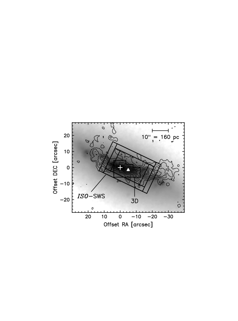
Figure 1:

Figure 2:

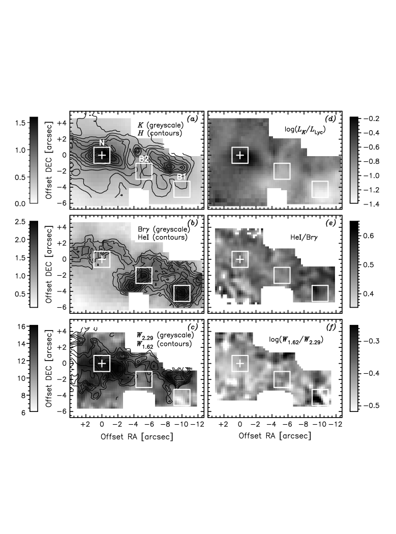
Figure 3:

Figure 4:

Figure 5:

Figure 6:

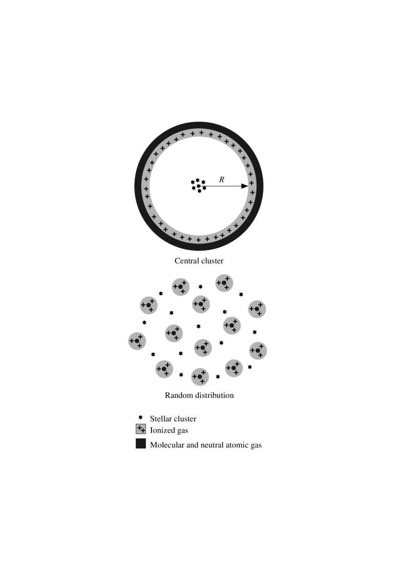
Figure 7:

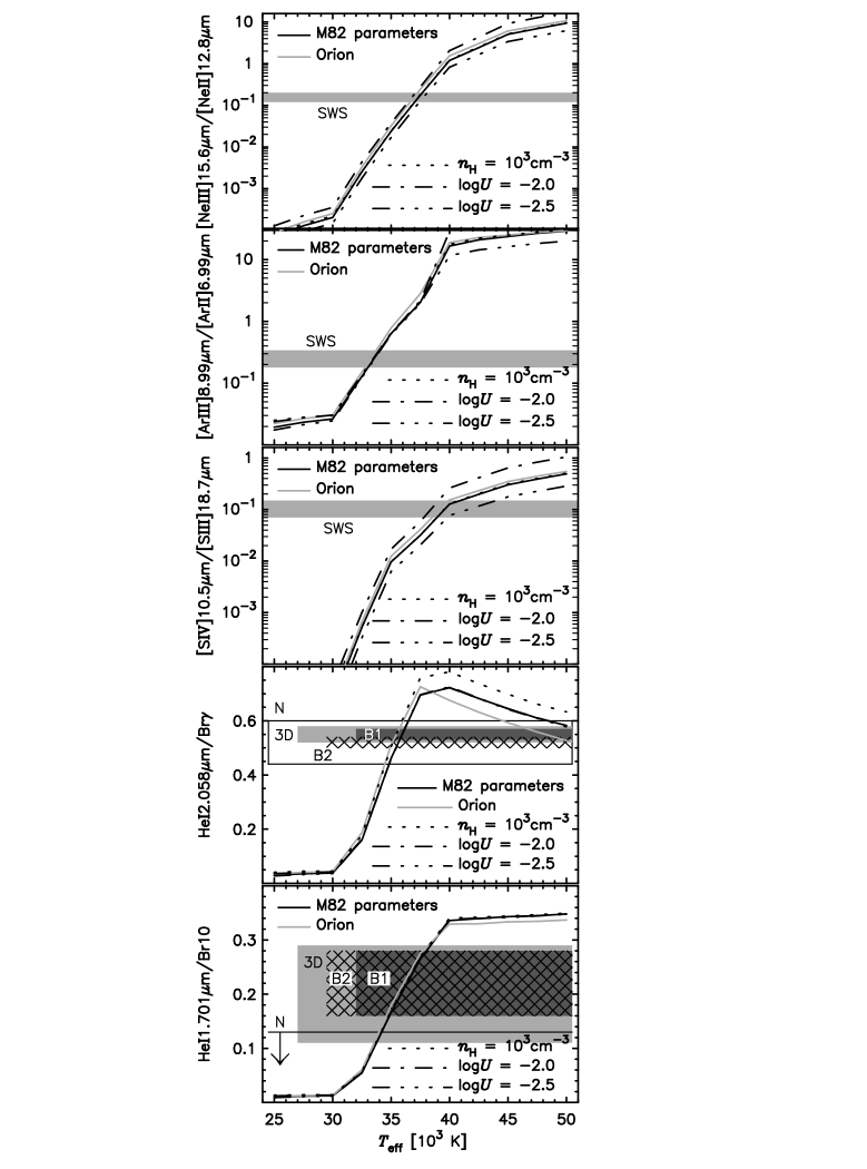
Figure 8:

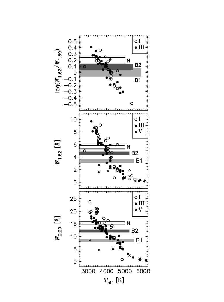
Figure 9:

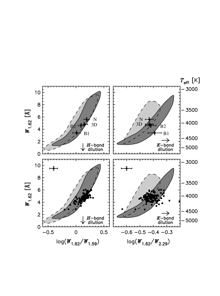
Figure 10:

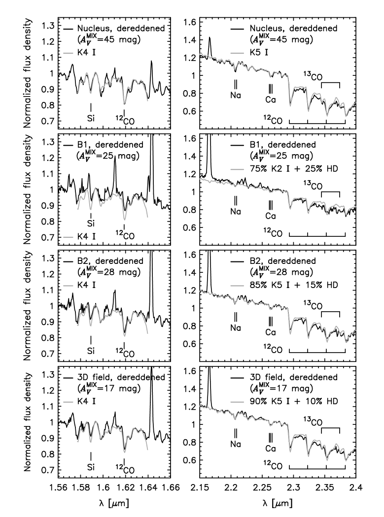
Figure 11:

Figure 12:

References

- Achtermann & Lacy (1995) Achtermann, J. M. & Lacy, J. H. 1995, ApJ, 439, 163
- Alexander et al. (1999) Alexander, T., Sturm, E., Lutz, D., Sternberg, A., Netzer, H., & Genzel, R. 1999, ApJ, 512, 204
- Allamandola et al. (1989) Allamandola, L. J., Tielens, A. G. G. M., & Barker, J. R. 1989, ApJS, 71, 733
- Allen & Kronberg (1998) Allen, M. L. & Kronberg, P. P. 1998, ApJ, 502, 218
- Bernlöhr (1992) Bernlöhr, K. 1992, A&A, 263, 54
- Black & van Dishoeck (1987) Black, J. H. & van Dishoeck, E. F. 1987, ApJ, 322, 412
- Blum et al. (1996) Blum, R. D., Sellgren, K., & DePoy, D. L. 1996, ApJ, 470, 864
- Bregman et al. (1995) Bregman, J. N., Schulman, E., & Tomisaka, K. 1995, ApJ, 439, 155
- Bruzual & Charlot (1993) Bruzual A., G. & Charlot, S. 1993, ApJ, 405, 538
- Butler & Zeippen (1994) Butler, K. & Zeippen, C. J. 1994, A&AS, 108, 1
- Cappi et al. (1999) Cappi, M., et al. 1999, A&A, 350, 777
- Carlstrom & Kronberg (1991) Carlstrom, J. E. & Kronberg, P. P. 1991, ApJ, 366, 422
- Clegg (1987) Clegg, R. E. S. 1987, MNRAS, 229, 31p
- Colbert et al. (1999) Colbert, J. W., et al. 1999, ApJ, 511, 721
- Dallier et al. (1996) Dallier, R., Boisson, C., & Joly, M. 1996, A&AS, 116, 239
- de Graauw et al. (1996) de Graauw, T., et al. 1996, A&A, 315, L49
- de Grijs et al. (2000) de Grijs, R., O’Connell, R. W., & Gallagher, J.S., III. 2000, in Proc. of the ESLAB Symp., Star Formation from the Small to the Large Scale, ed. F. Favata, A. A. Kaas, & A. Wilson (ESA SP-445), in press (astro-ph/9912109)
- Désert et al. (1990) Désert, F.-X., Boulanger, F., & Puget, J. L. 1990, A&A, 237, 215
- Devereux et al. (1987) Devereux, N. A., Becklin, E. E., & Scoville, N. Z. 1987, ApJ, 312, 529
- Dietz et al. (1986) Dietz, R. D., Smith, J., Hackwell, J. A., Gehrz, R. D., & Grasdalen, G. L. 1986, AJ, 91, 758
- Doane & Mathews (1993) Doane, J. S. & Mathews, W. G. 1993, ApJ, 419, 573
- Doherty et al. (1994) Doherty, R. M., Puxley, P. J., Doyon, R., & Brand, P. W. J. L. 1994, MNRAS, 266, 497
- Doherty et al. (1995) Doherty, R. M., Puxley, P. J., Lumsden, S. L., & Doyon, R. 1995, MNRAS, 277, 577
- Doyon et al. (1992) Doyon, R., Puxley, P. J., & Joseph, R. D. 1992, ApJ, 397, 117
- Draine (1989) Draine, B. T. 1989, in Proc. of the ESLAB Symp., Infrared Spectroscopy in Astronomy, ed. B. H. Kaldeich (ESA SP-290), 93
- Duffy et al. (1987) Duffy, P. B., Erickson, E. F., Haas, M. R., & Houck, J. R. 1987, ApJ, 315, 68
- Emerson (1988) Emerson, J. P. 1988, in Formation and Evolution of Low Mass Stars, ed. A. K. Dupree & M. T. V. T. Lago (Kluwer Academic Publishers), 21
- Ferland (1996) Ferland, G. J. 1996, Hazy, a Brief Introduction to Cloudy, University of Kentucky Department of Physics and Astronomy Internal Report
- Ferland (1999) Ferland, G. J. 1999, ApJ, 512, 247
- Förster et al. (1994) Förster, N. M., Doyon, R., Nadeau, D., & Rowlands, N. 1994, Astrophysics and Space Science Library, vol. 190, Infrared Astronomy with Arrays: the Next Generation, ed. I. S. McLean (Dordrecht: Kluwer), 509
- Förster Schreiber (2000) Förster Schreiber, N. M. 2000, AJ, 120, 2089
- Freedman & Madore (1988) Freedman, W. L. & Madore, B. F. 1988, ApJ, 332, L63
- Gaffney & Lester (1992) Gaffney, N. I. & Lester, D. F. 1992, ApJ, 394, 139
- Gaffney et al. (1993) Gaffney, N. I., Lester, D. F., & Telesco, C. M. 1993, ApJ, 407, L57
- Galavís et al. (1995) Galavís, M. E., Mendoza, C., & Zeippen, C. J. 1995, A&AS, 111, 347
- Gallagher & Smith (1999) Gallagher, J. S., III & Smith, L. J. 1999, MNRAS, 304, 540
- Genzel et al. (1998) Genzel, R., et al. 1998, ApJ, 498, 579
- Gillett et al. (1975) Gillett, F. C., Kleinmann, D. E., Wright, E. L., & Capps, R. W. 1975, ApJ, 198, L65
- Götz et al. (1990) Götz, M., McKeith, C. D., Downes, D., & Greve, A. 1990, A&A, 240, 52
- Gottesman & Weliachew (1977) Gottesman, S. T. & Weliachew, L. 1977, ApJ, 211, 47
- Greenhouse et al. (1997) Greenhouse, M. A., et al. 1997, ApJ, 476, 105
- Grevesse & Anders (1989) Grevesse, N. & Anders, E. 1989, in AIP Conf. Proc. 183, Cosmic Abundances of Matter, ed. C. J. Waddington (New York: AIP), 1
- Grevesse & Noels (1993) Grevesse, N. & Noels, A. 1993, in Origin and Evolution of the Elements, ed. N. Prantzos, E. Vangioni-Flam, & M. Casse (Cambridge: Cambridge Univ. Press), 15
- Haller & Rieke (1989) Haller, J. W. & Rieke, M. J. 1989, in IAU Symp. 136, The Center of the Galaxy, ed. M. Morris (Dordrecht: Kluwer), 487
- Ho & Filippenko (1996) Ho, L. C. & Filippenko, A. V. 1996, ApJ, 466, L83
- Holtzmann et al. (1992) Holtzmann et al. . 1992, AJ, 103, 691
- Houck et al. (1984) Houck, J. R., Shure, M. A., Gull, G. E., & Herter, T. 1984, ApJ, 287, L11
- Huang et al. (1994) Huang, Z. P., Thuan, T. X., Chevalier, R. A., Condon, J. J., & Yin, Q. F. 1994, ApJ, 424, 114
- Hummer & Storey (1987) Hummer, D. G. & Storey, P. J. 1987, MNRAS, 224, 801
- Hunt et al. (1999) Hunt, L. K., Malkan, M. A., Moriondo, G., & Salvati, M. 1999, ApJ, 510, 637
- Johnson et al. (1986) Johnson, C. T., Kingston, A. E., & Dufton, P. L. 1986, MNRAS, 220, 155
- Johnson & Méndez (1970) Johnson, H. L. & Méndez, M. E. 1970, AJ, 75, 785
- Joy & Lester (1988) Joy, M. & Lester, D. F. 1988, ApJ, 331, 145
- Kessler et al. (1996) Kessler, M. F., et al. 1996, A&A, 315, L27
- Kleinmann & Hall (1986) Kleinmann, S. G. & Hall, D. N. B. 1986, ApJS, 62, 501
- Kleinmann & Low (1970) Kleinmann, D. E. & Low, F. J. 1970, ApJ, 159, L165
- Koornneef (1983) Koornneef, J. 1983, A&A, 128, 84
- Kronberg et al. (1985) Kronberg, P. P., Biermann, P., & Schwab, F. R. 1985, ApJ, 291, 693
- Kronberg & Sramek (1985) Kronberg, P. P. & Sramek, R. A. 1985, Science, 227, 28
- Lançon et al. (1999) Lançon, A., Mouhcine, M., Fioc, M., & Silva, D. 1999, A&A, 344, L21
- Lançon & Rocca-Volmerange (1994) Lançon, A. & Rocca-Volmerange, B. 1994, Ap&SS, 217, 271
- Lançon et al. (1996) Lançon, A., Rocca-Volmerange, B., & Thuan, T. X. 1996, A&AS, 115, 253
- Landini et al. (1984) Landini, M., Natta, A., Oliva, E., Salinari, P., & Moorwood, A. F. M. 1984, A&A, 134, 284
- Larkin et al. (1994) Larkin, J. E., Graham, J. R., Matthews, K., Soifer, B. T., Beckwith, S., Herbst, T. M., & Quillen, A. C. 1994, ApJ, 420, 159
- Léger et al. (1989) Léger, A., d’Hendecourt, L., & Défourneau, D. 1989, A&A, 216, 148
- Lehnert et al. (1999) Lehnert, M. D., Heckman, T. M., & Weaver, K. A. 1999, ApJ, 523, 575
- Lester et al. (1990) Lester, D. F., Carr, J. S., Joy, M., & Gaffney, N. 1990, ApJ, 352, 544
- Lo et al. (1987) Lo, K. Y., Cheung, K. W., Masson, C. R., Phillips, T. G., Scott, S. L., & Woody, D. P. 1987, ApJ, 312, 574
- Lord (1992) Lord, S. 1992, NASA Techn. Mem. 103957, Ames Research Center, Moffet Field, CA
- Lord et al. (1996) Lord, S. D., Hollenbach, D. J., Haas, M. R., Rubin, R. H., Colgan, S. W. J., & Erickson, E. F. 1996, ApJ, 465, 703
- Lugten et al. (1986) Lugten, J. B., Watson, D. M., Crawford, M. K., & Genzel, R. 1986, ApJ, 311, L51
- Lutz (1999) Lutz, D. 1999, in The Universe as seen by ISO, vol. 2, ed. P. Cox & M.F. Kessler, (ESA SP-427), 623
- Lutz et al. (1998) Lutz, D., Kunze, D., Spoon, H. W. W., & Thornley, M. D. 1998, A&A, 333, L75
- Maoz et al. (1996) Maoz, D., Barth, A. J., Sternberg, A., Filippenko, A. V., Ho, L. C., Macchetto, F. D., Rix, H.-W., & Schneider, D. P. 1996, AJ, 111, 2248
- Mathis (1986) Mathis, J. S. 1986, PASP, 98, 995
- McCarthy et al. (1987) McCarthy, P. J., Heckman, T., & van Breugel, W. 1987, AJ, 92, 264
- McKeith et al. (1993) McKeith, C. D., Castles, J., Greve, A., & Downes, D. 1993, A&A, 272, 98
- McLeod et al. (1993) McLeod, K. K., Rieke, G. H., Rieke, M. J., & Kelly, D. M. 1993, ApJ, 412, 111
- Muxlow et al. (1994) Muxlow, T. W. B., Pedlar, A., Wilkinson, P. N., Axon, D. J., Sanders, E. M., & de Bruyn, A. G. 1994, MNRAS, 266, 455
- Neininger et al. (1998) Neininger, N., Guélin, M., Klein, U., García-Burillo, S., & Wielebinski, R. 1998, A&A, 339, 737
- Notni (1985) Notni, P. 1985, Astron. Nach., 306, 273
- O’Connell et al. (1994) O’Connell, R. W., Gallagher, J. S., III, & Hunter, D. A. 1994, ApJ, 433, 65
- O’Connell et al. (1995) O’Connell, R. W., Gallagher, J. S., III, Hunter, D. A., & Colley, W. N. 1995, ApJ, 446, L1
- O’Connell & Mangano (1978) O’Connell, R. W. & Mangano, J. J. 1978, ApJ, 221, 62
- Oliva & Origlia (1998) Oliva, E. & Origlia, L. 1998, A&A, 332, 46
- Oliva et al. (1995) Oliva, E., Origlia, L., Kotilainen, J. K., & Moorwood, A. F. M. 1995, A&A, 301, 55
- Olofsson & Rydbeck (1984) Olofsson, H. & Rydbeck, G. 1984, A&A, 136, 17
- Origlia et al. (1997) Origlia, L., Ferraro, F. R., Fusi Pecci, F., & Oliva, E. 1997, A&A, 321, 859
- Origlia et al. (1993) Origlia, L., Moorwood, A. F. M., & Oliva, E. 1993, A&A, 280, 536
- Osterbrock (1989) Osterbrock, D. E. 1989, Astrophysics of Gaseous Nebulae and Active Galactic Nuclei (Mill Valley, CA: University Science Books)
- Pauldrach et al. (1998) Pauldrach, A. W. A., Lennon, M., Hoffmann, T. L., Sellmaier, F., Kudritzki, R.-P., & Puls, J. 1998, in ASP Conf. Ser. 131, Properties of Hot Luminous Stars, ed. I. Howarth (San Francisco: ASP), 258
- Pedlar et al. (1999) Pedlar, A., Muxlow, T. W. B., Garrett, M. A., Diamond, P., Wills, K. A., Wilkinson, P. N., & Alef, W. 1999, MNRAS, 307, 761
- Pelan & Berrington (1995) Pelan, J. & Berrington, K. A. 1995, A&AS, 110, 209
- Pickles (1985) Pickles, A. J. 1985, ApJ, 296, 340
- Puxley (1991) Puxley, P. J. 1991, MNRAS, 249, 11p
- Puxley et al. (1989) Puxley, P. J., Brand, P. W. J. L., Moore, T. J. T., Mountain, C. M., Nakai, N., & Yamashita, T. 1989, ApJ, 345, 163
- Rieke & Lebofsky (1985) Rieke, G. H. & Lebofsky, M. J. 1985, ApJ, 288, 618
- Rieke et al. (1980) Rieke, G. H., Lebofsky, M. J., Thompson, R. I., Low, F. J., & Tokunaga, A. T. 1980, ApJ, 238, 24
- Rieke et al. (1993) Rieke, G. H., Loken, K., Rieke, M. J., & Tamblyn, P. 1993, ApJ, 412, 99
- Rieke & Low (1972) Rieke, G. H. & Low, F. J. 1972, ApJ, 176, L95
- Robbins (1968) Robbins, R. R. 1968, ApJ, 151, 511
- Roche et al. (1991) Roche, P. F., Aitken, D. K., Smith, C. H., & Ward, M. J. 1991, MNRAS, 248, 606
- Salama et al. (1997) Salama, A., et al. 1997, in First ISO Workshop on Analytical Spectroscopy, ed. A. M. Heras, K. Leech, N. R. Trams, & M. Perry (ESA SP-419), 17
- Salpeter (1955) Salpeter, E. E. 1955, ApJ, 121, 161
- Saraph & Tully (1994) Saraph, H. E. & Tully, J. A. 1994, A&AS, 107, 29
- Satyapal et al. (1995) Satyapal, S., et al. 1995, ApJ, 448, 611
- Satyapal et al. (1997) Satyapal, S., Watson, D. M., Pipher, J. L., Forrest, W. J., Greenhouse, M. A., Smith, H. A., Fisher, J., & Woodward, C. E. 1997, ApJ, 483, 148
- Schaeidt et al. (1996) Schaeidt, S. G., et al. 1996, A&A, 315, L55
- Schmidt-Kaler (1982) Schmidt-Kaler, T. 1982, in Landolt-Börnstein New Series, Vol. 2b, Astronomy and Astrophysics: Stars and Stellar Clusters, ed. K. Schaifers & H. H. Voigt (New York: Springer), 451
- Seaquist et al. (1985) Seaquist, E. R., Bell, M. B., & Bignell, R. C. 1985, ApJ, 294, 546
- Seaquist et al. (1996) Seaquist, E. R., Carlstrom, J. E., Bryant, P. M., & Bell, M. B. 1996, ApJ, 465, 691
- Seaquist et al. (1998) Seaquist, E. R., Frayer, D. T., & Bell, M. B. 1998, ApJ, 507, 745
- Seaquist et al. (1994) Seaquist, E. R., Kerton, C. R., & Bell, M. B. 1994, ApJ, 429, 612
- Shen & Lo (1995) Shen, J. & Lo, K. Y. 1995, ApJ, 445, L99
- Shields (1993) Shields, J. C. 1993, ApJ, 419, 181
- Shopbell & Bland-Hawthorn (1998) Shopbell, P. L. & Bland-Hawthorn, J. 1998, ApJ, 493, 129
- Simpson et al. (1995) Simpson, J. P., Colgan, S. W. J., Rubin, R. H., Erickson, E. F., & Haas, M. R. 1995, ApJ, 444, 721
- Smith et al. (1990) Smith, P. A., Brand, P. W. J. L., Puxley, P. J., Mountain, C. M., & Nakai, N. 1990, MNRAS, 243, 97
- Sternberg & Dalgarno (1989) Sternberg, A. & Dalgarno, A. 1989, ApJ, 338, 197
- Sturm et al. (2000) Sturm, E., Lutz, D., Tran, D., Feuchtgruber, H., Genzel, R., Kunze, D., Moorwood, A. F. M., & Thornley, M. D. 2000, A&A, 358, 481
- Stutzki et al. (1997) Stutzki, J., et al. 1997, ApJ, 477, L33
- Tacconi-Garman et al. (1996) Tacconi-Garman, L. E., Sternberg, A., & Eckart, A. 1996, AJ, 112, 918
- Telesco (1988) Telesco, C. M. 1988, ARA&A, 26, 343
- Telesco et al. (1991) Telesco, C. M., Campins, H., Joy, M., Dietz, K., & Decher, R. 1991, ApJ, 369, 135
- Telesco et al. (1993) Telesco, C. M., Dressel, L. L., & Wolstencroft, R. D. 1993, ApJ, 414, 120
- Telesco & Gezari (1992) Telesco, C. M. & Gezari, D. Y. 1992, ApJ, 395, 461
- Telesco & Harper (1980) Telesco, C. M. & Harper, D. A. 1980, ApJ, 235, 392
- Thornley et al. (2000) Thornley, M. D., Förster Schreiber, N. M., Lutz, D., Genzel, R., Spoon, H. W. W., Kunze, D., & Sternberg, A. 2000, ApJ, 539, 641
- Vacca et al. (1996) Vacca, W. D., Garmany, C. D., & Shull, J. M. 1996, ApJ, 460, 914
- van Buren & Greenhouse (1994) van Buren, D. & Greenhouse, M. A. 1994, ApJ, 431, 640
- van der Hulst et al. (1992) van der Hulst, J. M., Terlouw, J. P., Begeman, K., Zwitser, W., & Roelfsema, P. R. 1992, in ASP Conf. Ser. 25, Astronomical Data Analysis Software and Systems I, ed. D. M. Worall, C. Biemesderfer, & J. Barnes (San Francisco: ASP), 131
- Vanzi & Rieke (1997) Vanzi, L. & Rieke, G. H. 1997, ApJ, 479, 694
- Vanzi et al. (1996) Vanzi, L., Rieke, G. H., Martin, C. L., & Shields, J. C. 1996, ApJ, 466, 150
- Walker et al. (1988) Walker, C. E., Lebofsky, M. J., & Rieke, G. H. 1988, ApJ, 325, 687
- Waller et al. (1992) Waller, W. H., Gurwell, M., & Tamura, M. 1992, AJ, 104, 63
- Wamsteker (1981) Wamsteker, W. 1981, A&A, 97, 329
- Weitzel et al. (1996) Weitzel, L., Krabbe, A., Kroker, H., Thatte, N., Tacconi-Garman, L. E., Cameron, M., & Genzel, R. 1996, A&AS, 119, 531
- Whitmore & Schweizer (1995) Whitmore, B. C. & Schweizer, F. 1995, AJ, 109, 960
- Wild et al. (1992) Wild, W., Harris, A. I., Eckart, A., Genzel, R., Graf, U. U., Jackson, J. M., Russell, A. P. G., & Stutzki, J. 1992, A&A, 265, 447
- Willner et al. (1977) Willner, S. P., Soifer, B. T., Russell, R. W., Joyce, R. R., & Gillett, F. C. 1977, ApJ, 217, L121
- Wolfire et al. (1990) Wolfire, M. G., Tielens, A. G. G. M., & Hollenbach, D. 1990, ApJ, 358, 116
- Young et al. (1988) Young, J. S., Kleinmann, S. G., & Allen, L. E. 1988, ApJ, 334, L63
- Yun et al. (1993) Yun, M. S., Ho, P. T. P., & Lo, K. Y. 1993, ApJ, 411, L17
- Yun et al. (1994) Yun, M. S., Ho, P. T. P., & Lo, K. Y. 1994, Nature, 372, 530