Abstract

The challenge for optical detection of terrestial planet is the 25 magnitude brightness contrast between the planet and its host star. This paper introduces a new pupil design that produces a very dark null along its symmetry axis. By changing the shape of the pupil, we can control the depth and location of this null. This null can be further enhanced by combining this pupil with a rooftop nuller or cateye nuller and an aperture stop. The performance of the optical system will be limited by imperfections in the mirror surface. If the star is imaged with and without the nuller, then we can characterize these imperfections and then correct them with a deformable mirror. The full optical system when deployed on a 6 $\times$ 10 m space telescope is capable of detecting Earthlike planets around stars within 20 parsecs. For an Earthlike planet around a nearby stars (10 parsecs), the telescope can characterize its atmosphere by measuring spectral lines in the 0.3 - 1.3 micron range.

Submitted to Applied Optics

1. Introduction

The detection and characterization of Earthlike planets is one of a NASA’s highest priorities for the coming years. Currently, NASA’s plans focus on building large mid-infrared nulling interferometers that aim to detect thermal emission from planets and characterize the absorbtion lines in their atmosphere[1]. There is an alternative approach: a large optical telescope with a suitable coronagraph may be capable of detecting reflected light from the planets[2]. Since this large telescope would have a high quality optical surface, it would also be capable of 10 milliarcsecond imaging and would be a powerful instrument for near UV spectroscopy. There are a wide range of astronomical problems that could be addressed with a large optical/near UV space telescope[2, 3]. This large space telescope would be a boon to astrophysics!

Brown and Burrows[4] discuss searching for extrasolar planets with the Hubble Space Telescope. They emphasize the challenge for extrasolar planet searches: detecting the planet’s weak signal against the star’s bright light. They show that there were two dominant sources of noise in the observation: diffracted light due to the finite size of the aperature and scattered light due to imperfections in the mirror surface.

This paper is an attempt to design a system that is optimized for extrasolar planet detection. In section 2, I introduce a new pupil design and show that it can significantly reduce diffracted light along one axis of the system and discuss optimizing the pupil shape for terrestial planet finding. The optical system can be enhanced by combining this pupil with a coronagraph. In section 3, I discuss the scattered light problem and show how we can use a spectrograph placed along the symmetry axis of the system to characterize the mirror imperfections. A deformable mirror can correct these imperfections and reduce the stellar scattered light at the position of the planet. Section 4 discusses using this system to detect Earthlike planets around nearby stars and concludes the paper.

2. A New Pupil Design

A. Analytical Pupil Shape

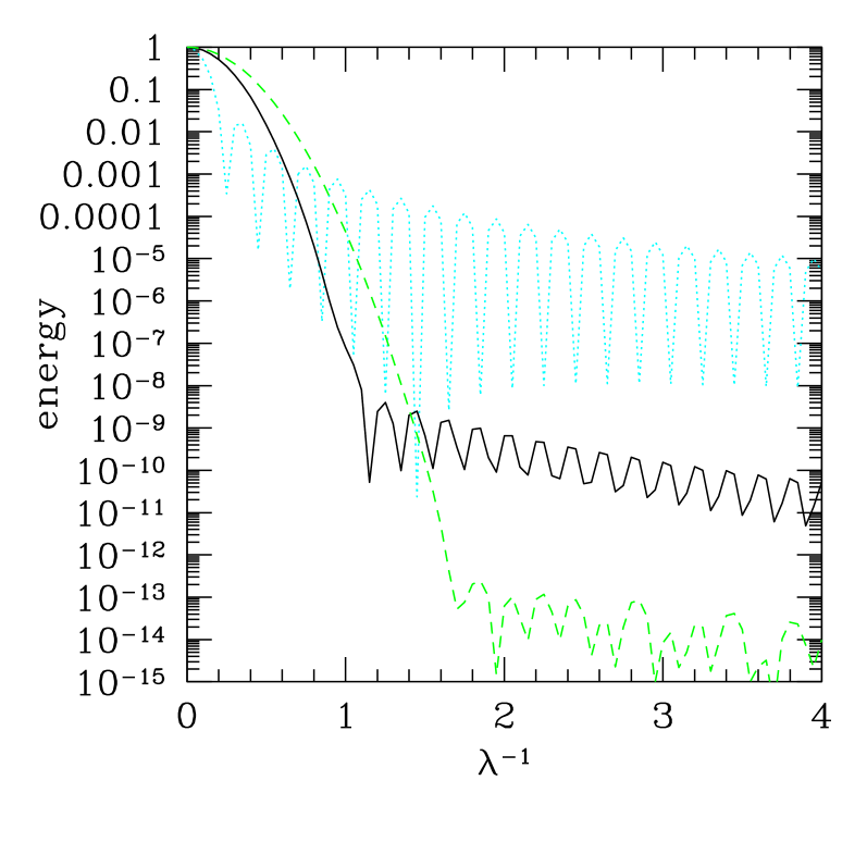
Fig. 1: Pupil diffraction pattern. The y axis shows the incident flux normalized to the central value for different pupil shapes. The x axis is measured in inverse wavenumbers (microns^-1) for a pixel seperated 0.1 arcseconds from the point source along the $\xi$ axis. The blue dotted line is for a circular aperature. The solid line is for a shaped aperature (equation 2) with $\alpha=2.7$. The green dashed line is for a shaped aperature with $\alpha=3.0$.

Fig. 2: Pupil Shape. This figure shows the two piece version of the pupil design. The axes are in meters

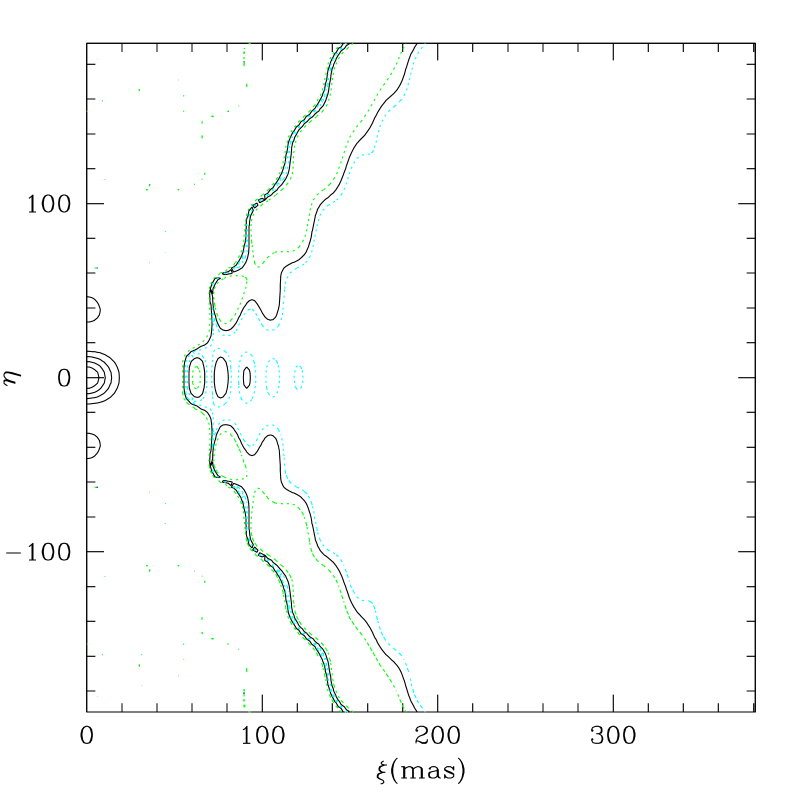
Fig. 3: Energy distribution. Near the peak, the solid contours show relative intensity levels of 0.2, 0.4, 0.6 and 0.8 times the peak intensity. Along the x-axis, the dotted, solid black, and dotted contours show regions with relative intensities of $10^{-9}$, $3\times 10^{-10}$ and $10^{-10}$

In this section, I introduce a pupil designed to minimize the diffracted light from the host star along its symmetry axis.

In the scalar optics limit, the diffraction pattern produced point source observed through a pupil at focus is the Fourier transform of its shape[5]:

$$I(\xi,\eta)=\int_{A(x,y)}dxdy\exp\left[ik\left(x\xi+y\eta\right)\right]$$ (1)

Throughout this paper, $k$ is the photon wavenumber, $\xi$ and $\eta$ are positions in the focal plane, and $x$ and $y$ are positions along the mirror surface. Along the $\xi$ axis, the optical response depends on the width of the pupil:

$$I(\xi,\eta)=\int dx\exp\left(ikx\xi\right)\left[y_{width}(x)-\frac{k^{2}\eta^{2}}{2}\int_{A(x,y)}y^{2}dy+\frac{k^{4}\eta^{4}}{24}\int_{A(x,y)}y^{4}dy+...\right]$$ (2)

where the odd terms in the expansion vanish as long as the pupil is symmetric about the x axis. For a circular aperature of radius, $R,$ $y_{width}(x)\;=\sqrt{R^{2}-x^{2}}$ and the diffraction pattern is the familiar Airy pattern. For a circular pupil, the energy recieved falls off as $\theta^{-3}$.

If the width of the pupil is close to a Gaussian,

$$y_{width}(x)=\exp\left[-(\alpha x/R)^{2}\right]-\exp(-\alpha^{2})$$ (3)

with $-R<x<R,$ then its diffraction pattern along the $\xi$ axis falls off much faster than that of a circular pupil:

$$I(\xi,0) = \int_{-R}^{R}dx\exp\left(ikx\xi\right)\left\{\exp\left[-(\alpha x/R)^{2}\right]-\exp(-\alpha^{2})\right\}$$

$$= {\pi\over 2}{R\exp\left({-k^{2}R^{2}\over 4\alpha^{2}}\right)\over\alpha}\left[{\rm erf}(\alpha+IKR/2\alpha))-{\rm erf}(\alpha-IkR/2\alpha)\right]$$

$$-\exp(-\alpha^{2})\frac{\sin(k\xi R)}{k\xi}$$

Figure 1 shows the energy recieved as a function of position in the focal plane for a circular aperature and a shaped pupil with several different values of $\alpha.$ Note the basic trade-off in the pupil design: if $\alpha$ is larger, then the null is deeper; however, the dark region starts at a larger radius.

If the pupil consists of a single opening, then equation (3) fully describes its shape. However, a two piece pupil is specified by an additional function, the position of the inner edge of the pupil (see figure 2). If the inner edge of the pupil is chosen so that

$$\int_{y_{inner}(x)}^{y_{inner}(x)+y_{width}(x)}y^{2}dy=\beta y_{width}(x),$$ (5)

then the null that is both deep and wide:

$$I(\xi,\eta)=I(\xi,0)(1-\beta k^{2}\eta^{2}+....)$$ (6)

Figure 2 shows the optical response of the two piece pupil and figure 3 shows an image of the two piece pupil.

The two piece pupil is well suited for a space telescope. The secondary mirror of the telescope and its support structure can sit in the dark region between the two pieces of the pupil. The primary mirror can consist of two pieces so that it can fold up and fit into fairing of the launch vehicle. In this folding mirror design, the fold also sits in the dark region between the pupil. With proper baffling, there should be not be significant scattered light from either the fold, the secondary or its support structure.

For a multi-mirror telescope, there are many possible higher order versions of this pupil that consist of multiple pieces. As long as the integrated width of the pupil satisfies equation (3) (or the appropriately optimized forms discussed in 2.3), the response of the pupil will be similar. In a multiple mirror system, not only can the first two terms in the expansion be supressed, but also the higher order terms in equation (2).

B. Combining the Pupil with a Coronagraph

The performance of the optical system can be enhanced by combining the pupil with the appropriate coronagraph. For example, the pupil could be combined with the achromatic interferocoronagraph[6]. In this coronagraph, the light from the star is split by a beam splitter into two equal intensity beams. One of the beampath experiences an additional reflection so that when the two beams are recombined, they are out of phase by $\pi$ and reflect around the symmetry axis. Since the diffraction pattern is symmetric, these two beams cancel and null out the star. In practice, there is a small optical path difference, $\Delta,$ between the two beampaths, so that the measured signal from the star is

$$I_{meas}(\xi,\eta)=\frac{1}{2}\left[1+\left(2\pi k\Delta\right)^{2}\right]I(\xi,\eta)-\frac{1}{2}I(-\xi,\eta)$$ (7)

Since the planet appears on only one side of the star, it is not nulled, instead, two images of the planet are detected.

By combining this nuller with the pupil design of section (2.1), we can combine the advantages of both and achieve a very deep null close to the star. If an X-shaped stop is placed in the focal plane in front of the nuller, then it will block most of the starlight from reaching the nuller. Thus, mirror imperfections in the nuller will not make a noticeable contribution to the scattered light reaching the CCD or spectrograph at the back end of the nuller.

Next, we consider a strawman optical system and assume that we can control the optical path difference in the nuller to better than $\lambda/6.$ This reduces the diffracted light from the star by 10^-3. When combined with a pupil designed to produce a null of depth 10^-7, the diffracted light from the star is now suppressed so that it is less than the light from the planet. With this combined system, we can detect with a 10 meter telescope, an Earth twin around star 10 parsecs away at all wavelengths shorter than 1.1 microns. In the next section, we will optimize the pupil shape and improve the wavelength coverage by 20%.

C. Optimizing the Pupil Shape

While the analytical pupil shape is a useful first step in designing the pupil, its shape is not optimal. the system performance can be improved by shaping the pupil so that it achieves a null of specified depth at all wavelengths shorter than a critical wavelength. I have done a two step optimization. In the first step, the width of the pupil was varied to obtain a deep null over as wide a wavelength range as possible along the axis of the pupil plane. In the second step, the inner edge of the pupil was varied to minimize the energy falling into a slit placed along the axis.

Using a simulated annealling routine, I have searched function space to find a function for the width of the mirror that creates a null of depth $10^{-7}$ at wavelengths shorter than 1.1 microns at angular seperation of 0.08 arcseconds. When this is combined with a nuller, the star’s light is suppressed by at least 10${}^{-10}.$ With this criterion, a 10 meter diameter telescope could detect the 1 micron water vapor line in an Earth-like planet around a Solar-type star at a distance of 10 parsecs and a seperation of 0.8 AU.

In the first optimization routine, I represent the mirror by its width at 64 points along a grid. At each step, the mirror shape is varied at each position by multiplying it by a random variable. The expectation value of this random variable is 1 and its variance is varied as a function of the iteration. For each pupil design, the program computes a quality parameter,

$$Q=\int_{k_{\min}}dk(I(k)-I_{\min})\;\Theta(I(k)-I_{\min})$$ (8)

where $I_{\min}$ is a fixed threshold (10${}^{-7})$ and $\;\Theta$ is the Heavyside function. If the quality factor for the new design is better than the current best design, the program always accepts it. If the quality factor is poorer than the current design, the program accepts it with a probability $\exp[-\left(Q_{new}-Q_{old}\right)/T]$, where the system temperature is slowly lowered through the calculation. The program ran for $10^{7}$ steps and showed only minor improvements during the final half of the run.

In the second step in the optimization routine, I minimized the energy falling into a 0.03 arcsecond wide slit along the axis for wavelengths shorter than 1.1 microns. I begin with the inner edge fixed so as to minimize the $\eta^{2}$ terms, where $\eta$ is th distance in the focal plane perpendicular to the slit (This leads to a large $\eta^{4}$ terms.) Using the same minimization routine, I now vary the inner edge of the profile.

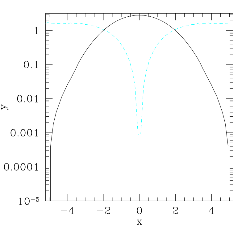
Fig. 4: Pupil Shape. The solid line shows the width of the pupil in meters as a function of x. The dashed line shows the position of the inner edge.

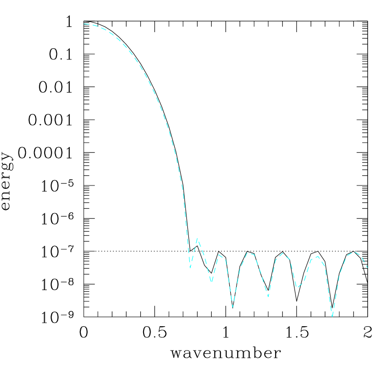
Fig. 5: The dashed line shows the amount of stellar light recieved into a 0.08 arc second wide slit located 0.1 arcseconds from the host star. The solid line shows the amount of stellar light recieved into a 0.005 arc second slit. Both lines are normalized to unity at wavenumber 0.

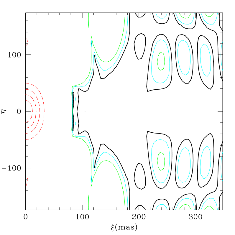
Fig. 6: The intensity response of the optimized pupil. The dotted red lines shows the shape of the central image. The contours are 0.2, 0.4, 0.6 and 0.8 of the peak intensity. The heavy black line encloses the region with intensity of less then $10^{-7}$ of the peak intensity. The light lines enclose regions with intensity less than $10^{-6.5}$ and $10^{-6}$ of the peak intensity. Recall that adding the nuller reduces these intensity by another factor of 10^-3. This plot is calculated for $\lambda=1.1$ microns, the longest target wavelength. The design has been optomized to minimize the light receieved into a 80 milliarcsecond wide slit along the axis.

Figure 4 shows the optimized pupil. Figure 5 shows the on-axis intensity as a function of wavenumber for the 10 meter system observing a planet at the seperation of 0.8. The dotted line in figure 5 shows the integrated energy recieved into a slit of width 0.02 arcseconds in a system using the split pupil design described in the previous section.Figure 6 shows the full two-dimensional response of the pupil.

3. Scattered Light Problem

The TPF optical system will not be perfect.Variations in the mirror surface will lead to phase and amplitude errors. Following [4], we can estimate these effects using scalar wave theory. Because of these errors, equation (1) is now modified

$$I(\xi,\eta,k) = \int_{A}dxdy\exp\left[ik(x\xi+y\eta)+ikG(x,y)\right]T(x,y)$$

$$= \tilde{A}(\xi,\eta)+k\tilde{G}(\xi,\eta)+\delta\tilde{A}(\xi,\eta)$$

where $T(x,y)$ is the transmission of the system and $G(x,y)$ describes variations in the mirror surface As long as he amplitude and phase errors are signficantly less than unity, we can approximate the effect of phase errors and amplitude errors as

$$\tilde{G}(\xi,\eta) = \int dxdy\exp\left[ik(x\xi+y\eta)\right]G(x,y)$$

$$\delta\tilde{A}(\xi,\eta) = \int dxdy\exp\left[ik(x\xi+y\eta)\right]\left[T(x,y)-\bar{T}\right]$$ (10)

where .$\bar{T}$ is the average transmission.  $\tilde{G}$ and $\delta\tilde{A}$ are complex functions.  It is convienent for the next subsection to split them into even and odd components.

While the engineering goal will be to minimize the errors in the mirror surface, the tolerances are so severe that on-orbit corrections will be essential. There are two complementary approaches to correcting the amplitude and phase errors:

• by slightly varying the shape of the aperture, we can cancel the amplitude errors along $\eta=0$ and can also cancel $\partial[\delta\tilde{A}(\xi,0)]/\partial\eta$

• a deformable mirror[7] can correct phase errors. Since the planned observations are primarily along a single axis, the deformable mirror does not need to correct errors over the full surface, but only along one dimension.

A detailed understanding of the mirror surface is essential for characterizing mirror imperfections. In the next section, we show how we can use observations with and without the nuller to characterize mirror errors

A. Using the nuller and spectrograph to measure errors

Here, we envision an optical system consisting of the optimized pupil, an X-shaped stop that blocks most of the scattered light, and a mirror that can send the residual star pattern either through a nuller or directly into a spectrograph. Note that because of the stop, very little light from the star enters the nuller, so that any optical errors in the mirrors in the nuller will not contribute significantly to the scattered light problem.

When the beam goes through the nuller, the spectrograph will measure

$$U_{nuller}(k,\xi) = \left|\frac{1}{2}\left[1+\left(2\pi k\Delta\right)^{2}\right]I(\xi,0)-\frac{1}{2}I(-\xi,0)\right|^{2}$$ (11)

$$= \left(k\tilde{G}_{odd}(\xi,0)+\delta\tilde{A}_{odd}(\xi,0)\right)^{2}$$

$$+2\left(2\pi k\Delta\right)^{2}\left(k\tilde{G}_{odd}(\xi,0)+\delta\tilde{A}_{odd}(\xi,0)\right)\left(\tilde{A}_{even}(\xi,0)+k\tilde{G}_{even}(\xi,0)+\delta\tilde{A}_{even}(\xi,0)\right)$$

$$+O(\Delta)^{4}$$

On the other hand, when the signal does not pass through the nuller, the detected signal will pick up both the odd and even terms.

Planets will also produce a response in the system. Unlike amplitude and phase errors, the effect of a planet is to produce a signal that is centered at a constant value of $v$ rather than a constant value of $k\xi.$When we combine all the effects, the number of photons detected by the optical system without the rooftop nuller is:

$$U_{nonuller}(k,\xi) = \left|I(\xi,0)\right|^{2}$$ (12)

$$= \left(\tilde{A}_{even}(\xi,0)+k\tilde{G}_{even}(\xi,0)+\delta\tilde{A}_{even}(\xi,0)\right)^{2}$$

If we ignore terms of order $\left(2\pi k\Delta\right)^{2},$ then we can immediately compute the amplitude and phase errors from equations (11) and (12).

4. Detectability of Earthlike Planets

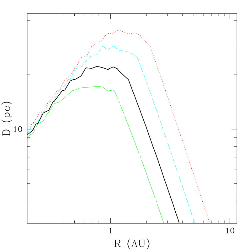
Fig. 7: This figure shows the time needed to detect a planet at the 5$\sigma$ level as a function of the distance to the host star and the distance from the host star to the target planet. The estimate includes the time needed to rotate the telescope to scan the solar system. The contours are for 3 Ks, 10 Ks, 30 Ks and 100 Ks integrations. This right hand panel is for a solar type star.

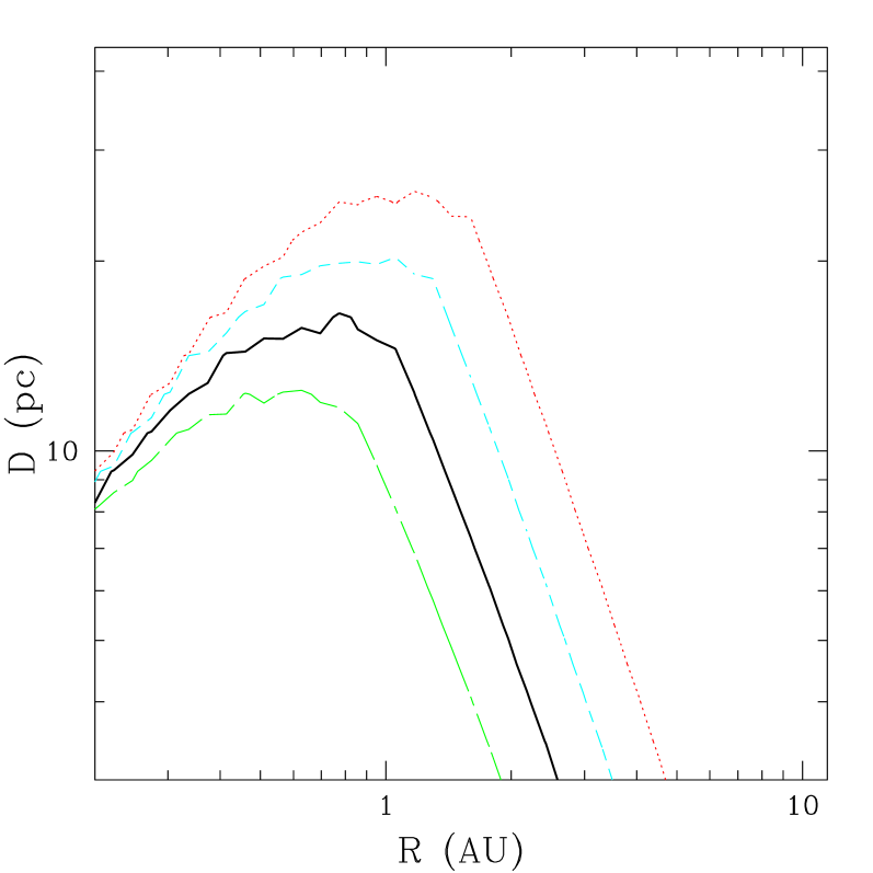
Fig. 8: This figure shows the time needed to detect a planet at the 5$\sigma$ level as a function of the distance to the host star and the distance from the host star to the target planet. The estimate includes the time needed to rotate the telescope to scan the solar system. The contours are for 3 Ks, 10 Ks, 30 Ks and 100 Ks integrations. This panel is for a K2 host star.

In this concluding section, I estimate the detectability of Earthlike planets around G and K stars based on a system built from two 3 x 10 meter mirrors and the system described in this note. In the estimate, I have assumed that the deformable mirrors have been able to correct mirrors at the level of $\lambda/10^{4},$ so that the amplitude of scattered light is comparable to the amplitude of the diffracted light (10^-10 peak value). With this level of supppresion, a planet 1 AU from the host star is as bright as the background light (Q=1 in the language of [4]). Since the brightness of the planet drops  as the distance from the host star increases, the Q value drops for planets further out in the system.

In estimating the signal-to-noise, I have assumed that the Earth-mass planet was at optimal phase and an albedo of 0.5 regardless of frequency for the planet’s surface. I assumed that the planet was monitored in U, B,V, R and I and combined the 5 bands to maximize the signal/noise. I assumed a 10% efficency for the full system at all wavelengths. For planets inside of 0.07 arcseconds, the shorter wavelengths are more important as diffracted light renders the longer wavelengths unusable. While the star is dimmer at short wavelengths, planets near the host star are brighter so that the two factors nearly cancel. Figure 7 shows estimates of time needed to detect the planet around a G2 and K2 star as a function of stellar distance and seperation. This figure shows that the proposed system appears to be a very effective planet finder, all of the G and K stars within 20 parsecs could easily be surveyed for Earthlike planets during the mission lifetime.

The proposed system should also be able to characterize the atmospheres of any detected planet. For an Earth twin around a star at a distance of 10 parsecs, the system should be capable of studying the atmosphere from 0.3 - 1.3 microns. This window contains a number of very important biotracers (O${}_{2},$O₃ and H₂O)[8].

A large optical telescope is a viable alternative to the traditional mid-infrared approach to planet detection. Building a large space telescope will be a challenging task; however, the potential scientific rewards are enormous in fields ranging from cosmology to planetary science.

5. Acknowledgements

This adventure into optical design would not have been possible without the advice of my colleagues. I have benefited from discussions with Jim Gunn, Norm Jarosik, Jeremy Kasdin, Michael Littman, Richard Miles, Sarah Seager and Ed Turner at Princeton. My fellows members of the Ball TPF team, in particular,John Bally, Torsten Boecker, Bob Brown, Chris Burrows, Christ Ftaclas, Steve Kilston, Charley Noecker, and Wes Traub, have provided insightful criticism and commments and have deepened my understanding of optics.

References

- [1] TPF Science Working Group, TPF reference mission, edited by C.A Beichman, N.J. Woolf and C.A Lindensmith, http://tpf.jpl.nasa.gov/mission/reference-mission.html
- [2] Ford, H., Angel, J.R.P., Burrows, Morse, J.A., Trauger, J.R. and Dufford, D.A., “HST to HST10x: A Second Revolution in Space Science”, http://eta.pha.jhu.edu/groups/hst10x/.
- [3] Shull, J.M., Savage, B.D., Morse, J.A., Neff, S.G., Clarke, J.T., Heckman, T., Kinney, A.L., Jenkins, E.B., Dupree, A.K., Baum, S.A. and Hasan, H., “The Emergence of the Modern Universe: Tracing the Cosmic Web”, Report of the UV/O Working Group to NASA, http://xxx.lanl.gov/astro-ph/9907101.
- [4] Brown, Robert A. & Burrows, Christopher J., “On the feasibility of detecting extrasolar planets by reflected starlight us ing the Hubble Space Telescope”, Icarus 87, 484-497 (1990).
- [5] Born, M & Wolf, M., Principles of Optics, Sixth Edition, Pergammon
- [6] Baudoz, P., Rabbia, Y. & Gay, J.,“ Achromatic inter fero coronagraphy I. Theoretical capabilities for ground-based observations”, Astronomy and Astrophysics Supplement, 141, p.319-329 (2000).
- [7] Malbet, F., Yu, J.W., and Shao, M., “High Dynamic Range Imaging Using a Deformable Mirror for Space Coronagraphy”, Publications of the Astronomical Society of the Pacific, 107, 386 - 394 (1995).
- [8] Traub, W.A. & Jucks, K.W., “Visible and Infrared Biomarkers: A Preliminary Comparision”, Ball-TPF progress report.