Intrinsic Shapes of Molecular Cloud Cores

Abstract

We conduct an analysis of the shapes of molecular cloud cores using recently compiled catalogs of observed axis ratios of individual cores mapped in ammonia or through optical selection. We apply both analytical and statistical techniques to de-project the observed axis ratios in order to determine the true distribution of cloud core shapes. We find that neither pure oblate nor pure prolate cores can account for the observed distribution of core shapes. Intrinsically triaxial cores produce distributions which agree with observations. The best fit triaxial distribution contains cores which are more nearly oblate than prolate.

1 Introduction

Molecular clouds are the sites of star formation in our Galaxy. Star formation occurs within dense cores in these clouds (Myers & Benson 1983; Benson & Myers 1989), as evidenced by their correlation with young stars (Beichman et al. 1986). While difficult to de-project, information about the intrinsic shapes of cores can yield insight into which physical processes control their evolution and thereby govern star formation.

Observational estimates of energy densities imply that many cores have magnetic, turbulent, and gravitational energies which are compatible with the cores being in virial equilibrium (Myers & Goodman 1988). Theoretical models of cloud equilibria routinely invoke axisymmetry, so that magnetically supported (Mouschovias 1976) or rotationally supported (e.g., Kiguchi et al. 1987) clouds, which are flattened in a preferred direction, assume an oblate shape. Such equilibria are analogous to axisymmetric oblate equilibrium models applied successfully to understand the structure of stars, planets, and accretion disks.

By analyzing the apparent shapes of 16 cores, Myers et al. (1991) concluded that the mean apparent axis ratio $\langle p\rangle$ $\approx$ 0.5 was consistent with oblate objects of intrinsic axis ratio $q\approx$ 0.1 - 0.3 and prolate objects with $q\approx$ 0.5. Based on a preference for less flattened objects and the suggestive elongation of some cores along elongated parent clouds, Myers et al. (1991) concluded that cores were more likely to be prolate axisymmetric objects than oblate axisymmetric objects. Ryden (1996) looked at the distribution of core shapes from several catalogs, including the Benson & Myers (1989) catalog of ammonia cores (41 objects) and the Clemens & Barvainis (1988) catalog of Bok globules. She concluded that the shape distribution of dense cores was more consistent with prolate rather than oblate objects, assuming that the cores were axisymmetric. The projected shapes of Bok globules were found to be consistent with either hypothesis, with oblate objects requiring an intrinsic mean axis ratio of 0.3, and prolate objects requiring a mean ratio of 0.5. Li & Shu (1996) have also pointed out that oblate objects with intrinsic axis ratio $\approx$ 0.3 can explain the observed $\langle p\rangle$ $\approx$ 0.5. Ciolek & Basu (2000) present a specific case of how an oblate cloud with such an axis ratio can fit the observations of a single core.

The apparent observational bias toward prolate axisymmetric objects has led to some models of equilibrium prolate objects (Tomisaka 1991; Fiege & Pudritz 2000) which require a dominant role for toroidal (rather than poloidal) magnetic fields, in order to maintain an equilibrium along the long axis. In practice, it is difficult to generate a model that can sustain a prolate geometry, as collapse along a poloidal field (parallel to the the long axis) results in oblate objects (Nakamura et al. 1995). Therefore, equilibrium prolate objects supported by toroidal field pressure require a constant source of significant magnetic helicity.

It has also been suggested that the apparently prolate shapes are an indication that cores are not in equilibrium (Fleck 1992). In fact, since many cores appear to be self-gravitating, it is natural to assume that gravitational motions (likely softened due to magnetic and/or turbulent support) are an important component in determining their evolution. An important feature of gravity is that it tends to enhance anisotropies in collapsing bodies (Mestel 1965; Lin, Mestel, & Shu 1965), so that unstable objects first collapse along one dimension, then break up into elongated objects within the sheet. While these objects may eventually break up into near-spherical fragments, this scenario implies that most objects have no intrinsic symmetry; thus a more general configuration is a triaxial, rather than an axisymmetric body. While studies of individual collapsing fragments often assume axisymmetry (e.g., Basu & Mouschovias 1994), as a consequence of equilibrium (or near-equilibrium) initial states, it is likely that such objects will not remain axisymmetric if the numerical restriction of axisymmetry is relaxed (e.g., see Nakamura & Hanawa 1997). Additionally, large scale turbulence in molecular clouds will also likely cause the initial states for collapse to deviate from perfect axisymmetry.

New surveys (Lee & Myers 1999; Jijina, Myers, & Adams 1999) have for the first time cataloged core properties for several hundred objects, allowing a more meaningful statistical analysis of core properties. Jijina et al. (1999) compiled a catalog of 264 dense cores from NH₃ observations, and Lee & Myers (1999) compiled a catalog of 406 dense cores from contour maps of optical extinction. With such data sets, the distribution of apparent projected core axis ratio $p$ (not just the mean value $\langle p\rangle$), can be used to constrain the intrinsic core shapes, similar to what has been done in the field of galaxy studies (see Lambas, Maddox & Loveday 1992; also discussion in Binney & Merrifield 1998)

In this paper, we conduct an analysis of the observed core shape distributions in order to determine their intrinsic shapes. We check the possibility that cores may be axisymmetric (prolate or oblate) objects in § 3, and consider the more general possibility of triaxial objects in § 4. A discussion and summary are given in §§ 5 and 6, respectively.

2 Theoretical Background

Any given oblate, prolate, or triaxial body, when viewed in projection, yields a distribution of observed projected axis ratios $\phi(p)$ arising from the different possible viewing angles. More generally, one often wishes to determine the distribution of intrinsic axis ratios based on the observed $\phi\left(p\right)$. Analytical methods have been developed to determine the intrinsic shapes of elliptical galaxies and globular clusters (for example, Sandage, Freeman & Stokes 1970; Binney 1978; Fall & Frenk 1983) from the observed $\phi(p)$, assuming intrinsically axisymmetric objects. We return to the axisymmetric case in § 3.

In general, a triaxial ellipsoid can be described by the equation

$$x^{2}+\frac{y^{2}}{\zeta^{2}}+\frac{z^{2}}{\xi^{2}}=a^{2},$$ (1)

where $a$ is a constant and $1\geq\zeta\geq\xi$. The geometrical analysis of Stark (1977) and Binney (1985) shows that such a body, when viewed in projection, has elliptical contours. Following Binney (1985), the projection of a triaxial body when viewed from an observing angle $(\theta,\phi)$ (where the angles are defined on an imaginary viewing sphere and have their usual meaning in a spherical coordinate system) is found using the quantities

$$A\equiv\frac{{\cos}^{2}\theta}{\xi^{2}}\left({\sin}^{2}\phi+\frac{{\cos}^{2}\phi}{\zeta^{2}}\right)+\frac{{\sin}^{2}\theta}{{\zeta}^{2}},$$ (2)

$$B\equiv\cos\theta\,\sin 2\phi\left(1-\frac{1}{\zeta^{2}}\right)\frac{1}{\xi^{2}},$$ (3)

and

$$C\equiv\left(\frac{{\sin}^{2}\phi}{\zeta^{2}}+{\cos}^{2}\phi\right)\frac{1}{\xi^{2}}.$$ (4)

The apparent axis ratio in projection then equals

$$p={\left(\frac{A+C-D}{A+C+D}\right)}^{1/2},$$ (5)

where $D\equiv\sqrt{{\left(A-C\right)}^{2}+B^{2}}$. Using these equations, one can construct probability distributions for the projected axis ratio, assuming a large number of randomly distributed viewing angles. If we assume that cores are either oblate or prolate axisymmetric objects, then the above equations simplify further since $\zeta=\xi$ for the prolate case, and $\zeta=1$ for the oblate case. Figure 1 shows an example of the distributions generated from these equations for axisymmetric cores. The oblate object is assumed to have an axis ratio of 0.3 and the prolate object an axis ratio of 0.5. Similar figures are presented in Binney & Merrifield (1998). These distributions peak at a value near the intrinsic axis ratio and then fall off rapidly. The oblate distribution (solid line) levels off to a near-constant value whereas the prolate distribution (dashed line) continues to decrease. The prolate distribution is also much more strongly peaked near its maximum. Both phenomena are related to the intuitive result that prolate (i.e., filamentary) objects appear elongated with an apparent axis ratio close to the true value when seen from most viewing angles. There is only a very rare chance of viewing them nearly along their long axis, from which they appear circular. Interestingly, both curves in Figure 1 have the same mean $\langle p\rangle$ $\approx 0.6$. This is evidence that simply fitting a model to the observed $\langle p\rangle$ may not yield reliable information about the intrinsic distribution of core shapes.

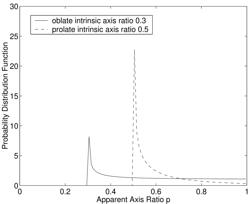
Figure 1: Probability density of observing the projected axis ratio $p$ assuming either a pure oblate intrinsic shape with an axis ratio of 0.3 or pure prolate intrinsic shape with an axis ratio of 0.5.

What would the observed distribution look like if cores were triaxial with particular values for the two axis ratios, $\zeta=b/a$ and $\xi=c/a$? Figure 2 shows the resulting distribution assuming a triaxial object with axis ratios of 0.3 and 0.8. Notice that the distribution, besides having peaks near 0.3 and 0.8, falls to zero at $p=1$, i.e., the body never appears circular in projection. Hence, the differences in shape of the predicted probability distribution, especially in the vicinity of $p=1$, act as an important discriminant in determining which intrinsic shapes best produce an observed distribution.

Figure 2: Probability density of observing the projected axis ratio $p$ assuming a triaxial shape with intrinsic axis ratios of 0.3 and 0.8.

The figures shown here were obtained by using a Monte Carlo program which calculates the expected observed distribution of axis ratios for an assumed intrinsic triaxial body (or distribution of triaxial bodies). The triaxial bodies can be prolate or oblate in special cases. The analytical expression (5) for $p$ is evaluated for a prescribed number of randomly placed viewing angles ($\theta,\phi$). This program is a modified version of one used by Dubinski & Carlberg (1991), and is used extensively to investigate triaxial shapes of cores in § 4.

3 Analytical Application to Ammonia Cores

In this section, we consider the axisymmetric assumption of either prolate or oblate cores. Now, if we assume axisymmetric cores with any intrinsic axis ratio $q$ equally likely, what is the expected distribution? Figure 3 shows the resulting distribution for intrinsic axis ratios distributed uniformly over the parameter space. This figure shows that for both axisymmetric shapes, the distribution peaks at large values of the projected axis ratio $p$; in other words, the projected probability distributions of objects with high $q$ (which have a strong peak at $p\gtrsim q$) dominate the overall distribution. This is clearly different than the actual observed distributions; (see Fig. 4 for example). Therefore, if these objects are axisymmetric, certain values of the axis ratios must be favored.

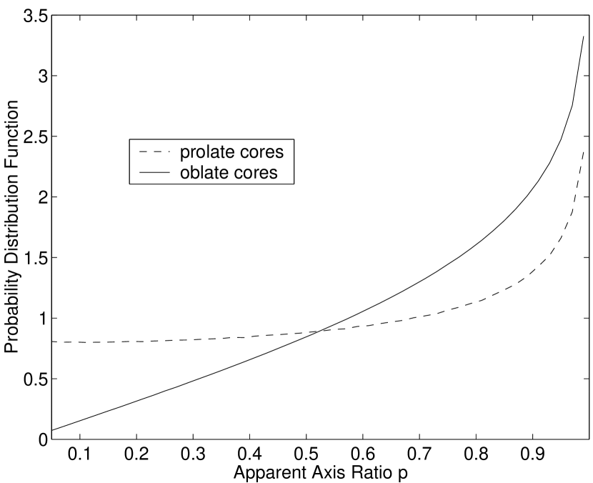
Figure 3: Probability density of observing the projected axis ratio $p$ assuming either an axisymmetric oblate (solid line) or prolate (dashed line) intrinsic shape and a uniform distribution of axis ratios.

Equations have been constructed which relate the observed distribution $\phi(p)$ to the distribution of intrinsic axis ratios $\psi(q)$, assuming either axisymmetric oblate or prolate objects (Fall & Frenk 1983). For pure oblate shapes,

$$\phi\left(p\right)=p\int^{p}_{0}dq\left(1-q^{2}\right)^{-\frac{1}{2}}\left(p^{2}-q^{2}\right)^{-\frac{1}{2}}\psi\left(q\right),$$ (6)

and for pure prolate shapes,

$$\phi\left(p\right)=p^{-2}\int^{p}_{0}dq\,q^{2}\left(1-q^{2}\right)^{-\frac{1}{2}}\left(p^{2}-q^{2}\right)^{-\frac{1}{2}}\psi\left(q\right).$$ (7)

Lambas et al. (1992) use a polynomial fit to the observed data, of the form

$$\phi\left(p\right)=c_{1}p+c_{3}p^{3}+c_{5}p^{5}.$$ (8)

They subsequently invert equations (6) and (7) to obtain

$$\psi_{\rm obl}\left(q\right)=\frac{2}{\pi}\left(1-q^{2}\right)^{1/2}\left(c_{1}+2c_{3}\,q^{2}+\frac{8}{3}c_{5}\,q^{4}\right)$$ (9)

and

$$\psi_{\rm pro}\left(q\right)=q^{-2}\left(1-q^{2}\right)^{1/2}\left(\frac{3}{2}c_{1}\,q^{3}+\frac{15}{8}c_{3}\,q^{5}+\frac{35}{16}c_{5}\,q^{7}\right),$$ (10)

using the methods of Fall & Frenk (1983). Their results show that both $\psi_{\rm obl}$ and $\psi_{\rm pro}$ become negative for values of $q$ greater than 0.9. They conclude that neither pure prolate or pure oblate models adequately describe the intrinsic shape of elliptical galaxies. A similar analysis by Ryden (1996), using a non-parametric kernel method, showed that the observed shape distribution of dense cores available in several catalogs were more consistent with intrinsically prolate (rather than oblate) spheroids, although the cores mapped in ammonia were inconsistent with both the prolate and oblate hypothesis.

Here, we also apply an analytical inversion method, assuming axisymmetry, to the recent survey by Jijina et al. (1999) of dense cores mapped in ammonia. Based on the size and estimated uncertainties of the Jijina et al. data set, a histogram of the observed axis ratios $p$ is created with 10 bins to sample the data adequately. The observations are then fit with polynomials of various degrees in order to find the best fit. Following the approach by Lambas et al. (1992), we find that an odd polynomial of degree 5 represents a good fit to the data, with $c_{1}=1.75,c_{3}=5.28$, and $c_{5}=-6.97$. Figure 4 shows the histogram of the original data and the polynomial fit. Equations (9) and (10) are then evaluated using this polynomial fit. The resulting distributions $\psi_{\rm obl}$ and $\psi_{\rm pro}$ are displayed graphically in Figure 5. For both the assumptions of oblate cores and prolate cores, the predicted intrinsic distribution of axis ratios becomes negative for large values of $q$. Clearly this resulting distribution is unphysical. Either the initial assumption of axisymmetry is incorrect, or errors in one or more of the binning, polynomial fits, or observations have caused this unphysical result. Also, for this analysis to be applicable, the cores must be randomly oriented in space. For specific star forming regions there may be some preferred orientation of the cores; however, this catalog samples many areas of the sky and is composed of hundreds of data points, so we assume that the cores are randomly oriented.

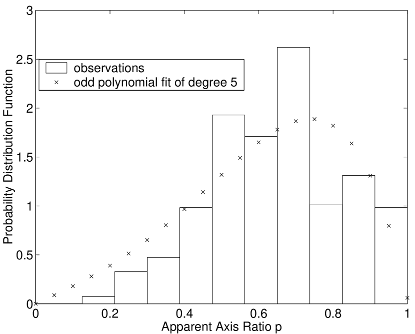
Figure 4: A comparison of the binned data set (a normalized histogram) of projected axis ratios for the cores mapped in ammonia (Jijina et al. 1999) with the odd polynomial fit.

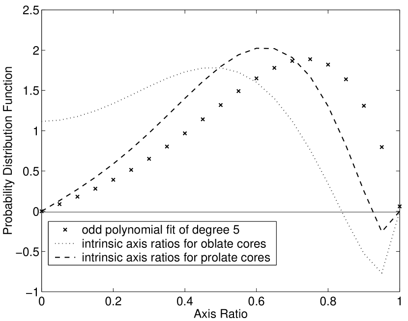
Figure 5: The analytically derived intrinsic axis ratio distributions $\psi_{\rm obl}$ (dotted line) and $\psi_{\rm pro}$ (dashed line) for the Jijina et al. (1999) data. The polynomial fit to the observed axis ratio distribution (crosses) is also shown.

To estimate the effect of observational, binning, and polynomial fitting errors, we apply a technique known as boot-strapping, which requires removing and adding data to various bins in the data set. We are most interested in changes in the values of the projected axis ratios $p\gtrsim 0.8$, which determine whether or not the values of the intrinsic axis ratio $q$ can become positive. Removing data in these bins produces oblate and prolate fits which are more negative. Adding data at large $p$ increases the probability distribution function for large $q$; however, we find that adding up to 20% more data values of $p$ in the range from 0.8 to 0.9 and 0.9 to 1.0 produces intrinsic distributions which still remain negative for large values of $q$. We conclude that neither pure oblate nor pure prolate distributions can reproduce the observed axis ratios.

4 Analysis of Triaxial Cores

Since we reject the possibility that cores are axisymmetric in § 3, we now consider a more general shape for cores. If we assume, for example, that these objects are triaxial with any intrinsic axis ratio equally likely, what is the expected observed distribution? Figure 6 shows the resulting distribution from our Monte Carlo program, assuming triaxial cores with axis ratios $\zeta$ and $\xi$ distributed uniformly in the range [0,1]. (Also shown is a normalized histogram of the observed ammonia cores.) This distribution turns down towards $p=1$, as all distributions for individual triaxial bodies do, and is therefore a better fit to observations than a uniform distribution of axisymmetric objects (see Fig. 3). However, it is still not a good fit to the observations. The distribution greatly overestimates the number of objects with axis ratios $\leq 0.4$, does not fit the peak of the observed distribution near 0.6, and underestimates the number of objects with axis ratios $\geq 0.9$. Therefore, if cores are triaxial in shape, certain values of axis ratios must be preferred.

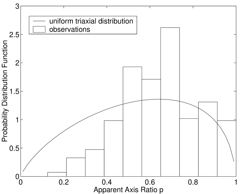
Figure 6: Probability density of observing the projected axis ratio $p$ assuming a triaxial shape for a uniform distribution of axis ratios. Also shown is the binned data set (Jijina et al. 1999) of the cores mapped in ammonia for comparison.

We conduct an investigation in order to determine the most likely values of the axis ratios $\zeta$ and $\xi$ for a distribution of triaxial shaped cores. We assign a Gaussian distribution for each axis ratio $\zeta$ and $\xi$, with a mean in the range $[0,1]$, and standard deviation $\sigma$ typically equal to 0.1, consistent with our use of 10 bins to sample the data. We did test a range of $\sigma$’s from 0.05 to 0.2, and present the best fits for $\sigma=0.1$ in this paper. We find that our conclusions do not change significantly within this range of $\sigma$ values. The drawback to using relatively large $\sigma\gtrsim 0.2$ is that a relatively large fraction of the Gaussian distribution falls outside the allowed range $[0,1]$. We tested several different ways to deal with these values: (1) we set values less than zero to zero and values greater than one to one; (2) we removed all numbers outside of the range of zero to one; (3) we rejected numbers which fell outside of the range of zero to one and repeatedly generated a new random number until one between zero and one was obtained. None of these methods is completely satisfactory since Gaussian distributions modified by these methods clearly have different means and standard deviations than originally specified. We believe that it is not very meaningful to test Gaussian distributions with larger values of $\sigma$ than 0.2 especially near the end-points of our parameter space. For example, a Gaussian distribution centered at 0.8 with a $\sigma$ of 0.2 has $\approx$ 16% of the data $>1$. If one simply truncates the values $>1$, the new resultant distribution is centered at 0.7 with a standard deviation of 0.16. For similar reasons, we limit the $\sigma=0.1$ analysis to the range of axis ratios [0.1,0.9].

In order to find the best fit intrinsic distribution of triaxial bodies, distributions of axis ratios with peak values $\xi_{0}$ and $\zeta_{0}$ (for a given $\sigma$) are input into the Monte Carlo program described in § 2. We typically employ at least $10^{4}$ viewing angles to calculate the projected distribution for each pair of axis ratios, and at least $10^{4}$ axis ratios for each Gaussian distribution. This is more than sufficient for comparison with data sets sampled in only 10 bins. The program produces the expected observed distribution which results from the assumed intrinsic distributions. We compare this output with the observed data sets of both Jijina et al. (1999) and Lee & Myers (1999). The best fits are determined by comparing with the data bins and calculating the $\chi^{2}$ value. Figure 7 and Figure 8 show 2-dimensional plots of the inverse $\chi^{2}$ values for the Jijina et al. data and the Lee & Myers data, respectively. Both data sets are fit best by a triaxial distribution with $\xi_{0}$ just below the observed mean $\langle p\rangle$ and $\zeta_{0}$ close to unity. The Jijina et al. data set is best fit by distributions with axis ratios $(\xi_{0},\zeta_{0})=(0.5,0.9)$, and the Lee & Myers data set is best fit by values $(\xi_{0},\zeta_{0})=(0.3,0.9)$. For comparison, Jijina et al. (1999) calculate a mean projected aspect ratio $\langle p\rangle^{-1}\approx 1.5$, or equivalently $\langle p\rangle\approx.67$. Lee & Myers state a value of $\langle p\rangle^{-1}\approx 2.4$, or equivalently $\langle p\rangle\approx.42$ for their data set. (For the Lee & Myers data set, we calculate a mean projected aspect ratio of 2.0 directly from their data set. It is unclear what the reason for this discrepancy is.) Nevertheless, our main conclusions are clear: (1) a triaxial distribution rather than an axisymmetric distribution can best produce the observed distribution of shapes; (2) the most likely distribution of triaxial shapes has more near-oblate objects than near-prolate ones, since $\zeta_{0}$ is always close to 1. (Formally, one may say that the cores are more nearly oblate if $\zeta_{0}>\text@frac{1}{2}[1+\xi_{0}]$.)

The differences in the best fit axis ratios ($\xi_{0},\zeta_{0}$) for the two data sets may simply reflect differences in the intrinsic shape of these cores when mapped in ammonia lines compared to optical observations. Lee & Myers (1999) state that the optical maps trace regions of mean density $n\simeq(6-8)\times 10^{3}$ cm^-3, which is slightly lower than the $n\gtrsim 10^{4}$ cm^-3 sampled in ammonia maps. Hence, the greater mean elongation (lower $\langle p\rangle$) of the optically selected cores, which results in a lower best-fit $\xi_{0}$, may be related to the theoretical result that outer density contours of core models are often more elongated than inner ones (e.g., Fiedler & Mouschovias 1993). This is due to the isotropic thermal pressure support being relatively more important on smaller scales.

In order to test the robustness of our result, we remove 20% of the data in each sample randomly and recalculate the $\chi^{2}$ values. This is repeated 10 times for each data set. Each such simulation with the Jijina et al. (1999) data set continues to have a best fit at mean axis ratios 0.5 and 0.9. The Lee & Myers data has a best fit with one mean axis ratio 0.3 in all cases, and the other in the range 0.7 to 0.9, with a mean of 0.83.

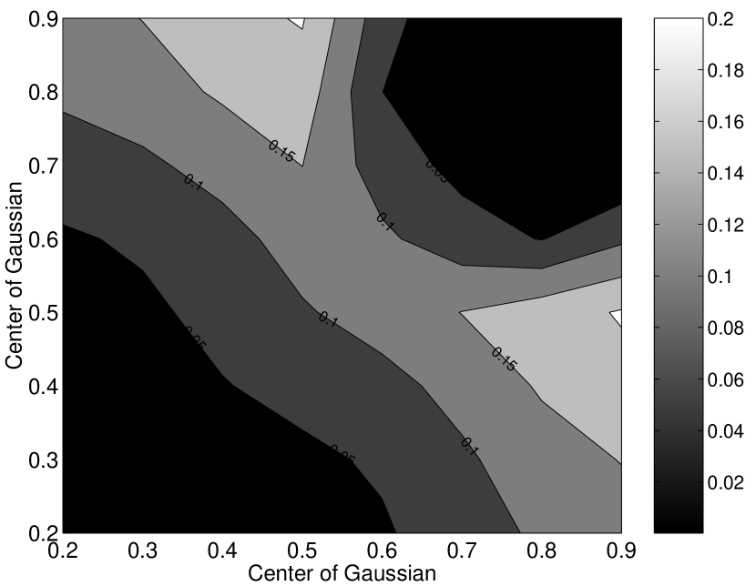
Figure 7: A 2-dimensional plot of inverse $\chi^{2}$ values for triaxial core shape models for the Jijina et al. (1999) data. Note the symmetry of the figure about the line along which the two centers of the axis distributions are equal. For any point in the figure, the smaller axis ratio corresponds to $\xi_{0}$ and the larger to $\zeta_{0}$.

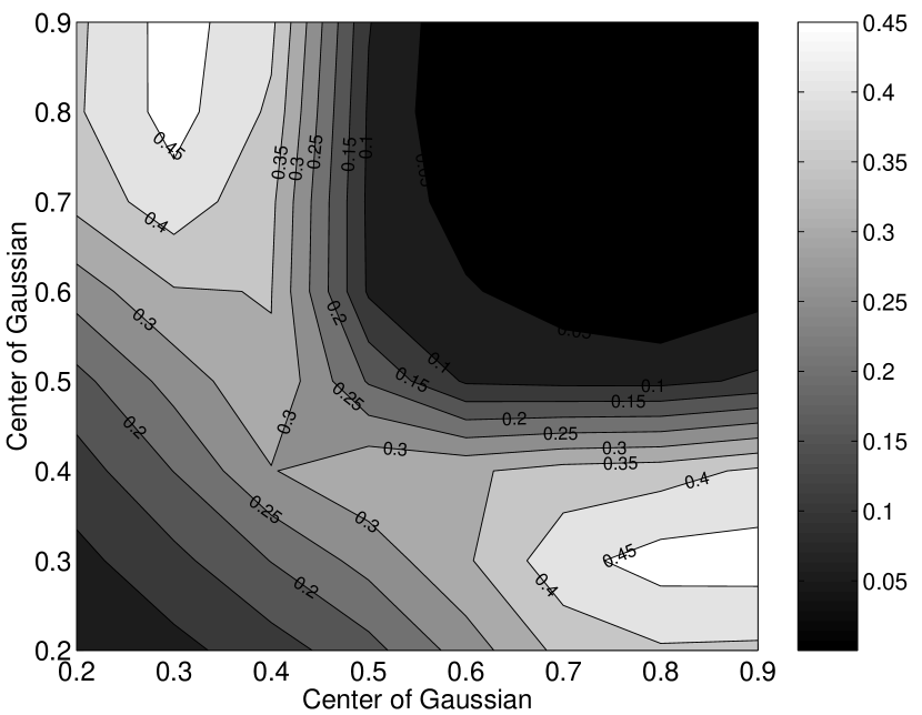
Figure 8: A 2-dimensional plot of inverse $\chi^{2}$ values for triaxial core shape models for the Lee & Myers (1999) data.

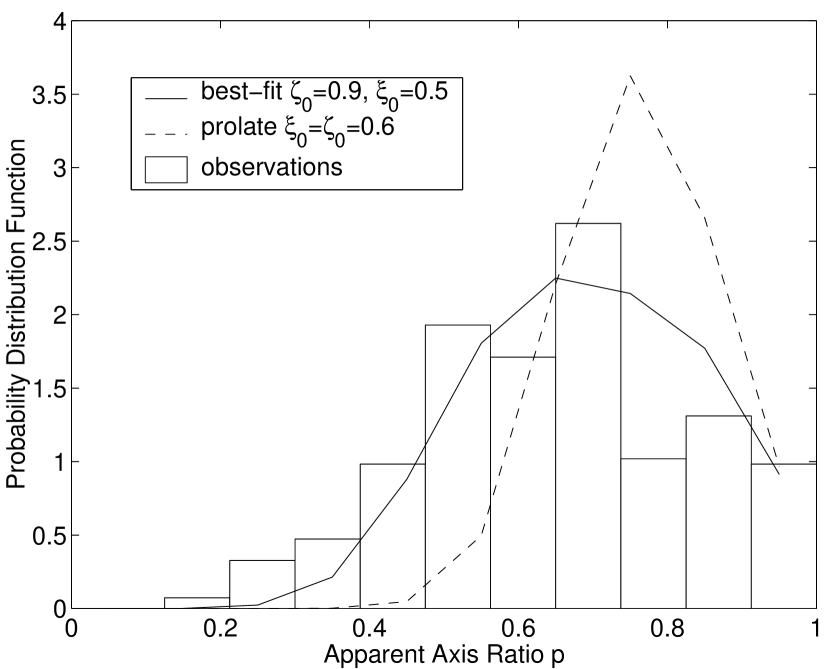
Figure 9: A comparison of the observed axis ratios from the ammonia data set (Jijina et al. 1999) with the best fit assuming triaxial cores (solid line). Also shown is the projected distribution for intrinsic distributions with $\zeta_{0}=\xi_{0}$, i.e., cores which are more prolate in shape (dashed line). Both calculated distributions are binned in ten intervals, as is the data set.

Finally, Figure 9 presents a comparison of the best fit of the projected distribution (based on the $\chi^{2}$ values) with the Jijina et al. (1999) data. For further comparison, we also display the best fit among the projected distributions that arise from intrinsic distributions with $\zeta_{0}=\xi_{0}$, i.e., that emphasize prolate shapes. Notice that such a distribution does not fit the data well; the distribution is much too strongly peaked. This strong peaking can be traced back to the very strongly peaked nature of the observed distribution from any single prolate object (see Fig. 1).

5 Discussion

Why are triaxial bodies favored in this analysis? A very important factor in analyzing the the projected distribution $\phi(p)$ is its shape near $p=1$. The pronounced drop towards $p=1$ (see Fig. 4) favors triaxial bodies since all such bodies viewed in projection yield $\phi(p)\rightarrow 0$ as $p\rightarrow 1$ (see Fig. 2). Within the confines of the axisymmetric assumption, a decrease in $\phi(p)$ towards unity favors prolate over oblate objects (Ryden 1996) because the former are less likely to appear nearly circular in projection (see Fig. 1). However, once the axisymmetric restriction is dropped, all triaxial clouds can satisfy the need for a decrease in $\phi(p)$ towards unity. In this case, the broad peak in the distribution and the fact that a significant number of cores with $p\approx 1$ are still present favors the near-oblate triaxial clouds rather than the near-prolate ones. As exhibited in Figure 1 and Figure 9, prolate clouds (or distributions that emphasize prolate clouds) yield projected distributions that are too sharply peaked and underestimate the data points near $p=1$.

It is interesting to note that our results are qualitatively similar to the conclusions of Lambas et al. (1992) and Binney & Merrified (1998) that triaxial, but more nearly oblate, shapes are always preferred when de-projecting elliptical galaxy shapes. This is despite the different physical forces at play in the support of galaxies versus cloud cores, though both represent self-gravitating systems.

While a triaxial shape for dense cores clearly favors non-equilibrium phenomena influencing their evolution (see discussion in § 1), the near-oblateness also implies that the cores may not be particularly far from equilibrium. Oblateness is theoretically consistent with models of magnetically and/or rotationally supported equilibria (e.g., Mouschovias 1976; Tomisaka, Ikeuchi, & Nakamura 1989). In contrast, prolate equilibria have proven exceedingly difficult to construct, requiring exotic effects whose presence has not been established (see § 1). Near-equilibrium and near-oblate cores are also consistent with the overwhelming observational evidence for near virial equilibrium in cores (e.g., Myers & Goodman 1988), and the evidence for preferential flattening of cores along the direction of the mean magnetic field, shown by the correlation $B\propto\rho^{1/2}$ between magnetic field strength $B$ and density $\rho$ (see Crutcher 1999 and discussion in Basu 2000). Most generally, this preferential flattening of cores along one direction, parallel to the mean magnetic field, favors an oblate (or near-oblate) geometry, in which one direction is especially flattened; in a prolate geometry, two perpendicular directions must have the same degree of flattening.

If cores are indeed flattened along one preferred direction which corresponds to that of the mean magnetic field, one may infer the distribution of observed offset angles $\Psi$ between the projected magnetic field direction and the projected minor axis of the core. As shown by Basu (2000), a triaxial body seen in projection will allow a finite probability of viewing any nonzero $\Psi$, although there will be a bias toward $\Psi=0$. Here, we calculate a probability distribution for viewing $\Psi$ using our best fit intrinsic triaxial shape distribution, and assuming the shortest axis of any core corresponds to the mean magnetic field direction. (See Basu 2000 for a discussion of how $\Psi$ is calculated.) Figure 10 shows the resulting probability distribution for an intrinsic axis ratio distribution with peaks at 0.5 and 0.9, and $\sigma=0.1$. For comparison, the distribution of $\Psi$ for a uniform distribution of triaxial bodies is also shown. There is not a big difference between the two, although the best fit distribution, which emphasizes near-oblate clouds, yields a smaller probability for observing large $\Psi$ (note that in the oblate limit, a cloud only allows observations of $\Psi=0$). These probability distribution functions act as a prediction for future distributions of $\Psi$ obtained through submillimeter polarimetry of a large number of dense cores (e.g., see Matthews & Wilson 2000; Ward-Thompson et al. 2000 for a few recent measurements). The prediction of a bias toward $\Psi=0$ due to preferential flattening along the mean magnetic field direction is consistent with the observed $B\propto\rho^{1/2}$ relation and contrasts with that expected if turbulent motions dominate magnetic forces during core formation, in which case there should be no correlation of $\Psi$ toward any value.

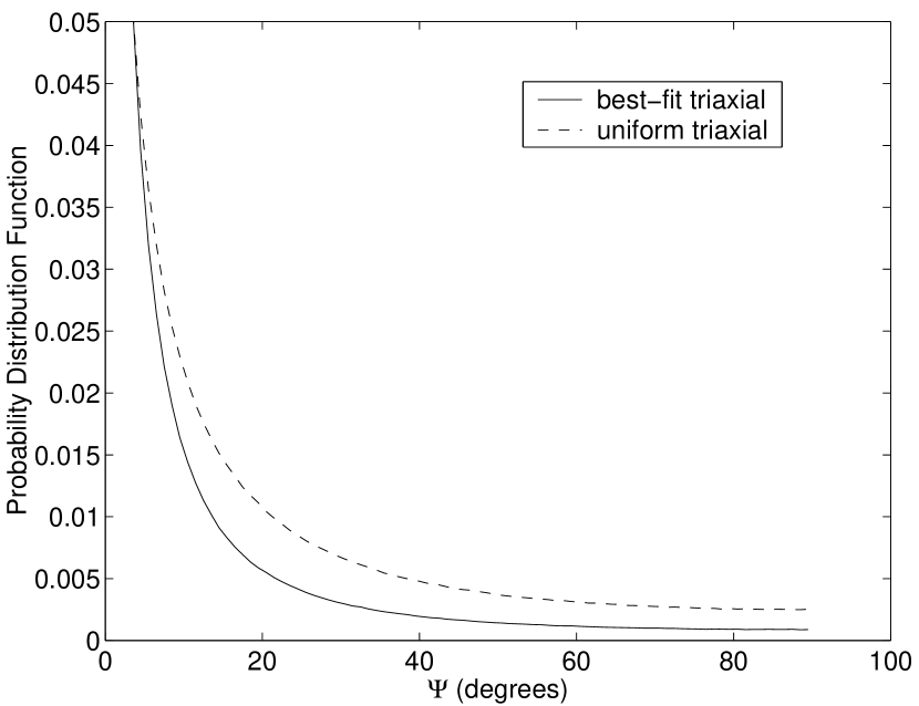
Figure 10: Probability density of observing an offset angle $\Psi$ between the projected magnetic field direction and projected minor axis for a distribution of triaxial bodies for which the short axis coincides with the mean magnetic field direction. We use either our best-fit (to the Jijina et al. data set) distribution of axis ratios (solid line) or a uniform distribution of axis ratios (dashed line).

6 Summary

In § 3 we considered the assumption of pure axisymmetric oblate or prolate cores analytically. We found that this assumption led to unphysical results, so we rejected the hypothesis that cores are axisymmetric. In § 4, we investigated triaxial cores statistically. We found that for the Jijina et al. (1999) data set, intrinsic mean axis ratios of $0.5$ and $0.9$ best fit the observations, and for the Lee & Myers (1999) data set, mean axis ratios of $0.3$ and $0.9$ best fit the observations, for assumed Gaussian distributions with standard deviation $\sigma$ of 0.1. Additionally, choosing $\sigma$ in the range [0.05,0.2] gives essentially the same result.

It is worth reiterating that we find that one of the best fit intrinsic axis ratios is always quite a bit larger than the other axis ratio, which suggests that cores are preferentially flattened in one direction, and close to oblateness. While triaxiality implies a non-equilibrium state for most dense cores, the near-oblate shape implies that the initial conditions for collapse may not be particularly far from equilibrium.

References

- (1)
- (2) Basu, S. 2000, ApJ, 540, L103
- (3)
- (4) Basu, S., & Mouschovias, T. Ch. 1994, ApJ, 432, 720
- (5)
- (6) Beichman, C. A., Myers. P. C., Emerson, J. P., Harris, S., Mathieu, R., Benson, P. J., & Jennings, R. E. 1986, ApJ, 307, 337
- (7)
- (8) Benson, P. J., & Myers, P. C. 1989, ApJS, 71, 89
- (9)
- (10) Binney, J. 1978, MNRAS, 183, 501
- (11)
- (12) Binney, J. 1985, MNRAS, 212, 767
- (13)
- (14) Binney, J., & Merrifield, M. 1998, Galactic Astronomy, (Princeton: Princeton Univ. Press)
- (15)
- (16) Ciolek, G. E., & Basu, S. 2000, ApJ, 529, 925
- (17)
- (18) Crutcher, R. M. 1999, ApJ, 520, 706
- (19)
- (20) Dubinski, J., & Carlberg, R. G. 1991, ApJ, 378, 496
- (21)
- (22) Fall, S. M., & Frenk, C. S. 1983, AJ, 88, 1626
- (23)
- (24) Fiedler, R. A., & Mouschovias, T. Ch. 1993, ApJ, 415, 680
- (25)
- (26) Fleck, R. C. Jr. 1992, ApJ, 401, 146
- (27)
- (28) Jijina, J., Myers, P. C., & Adams, F. C. 1999, ApJS, 125, 161
- (29)
- (30) Kiguchi, M., Narita, S., Miyama, S. M., & Hayashi, C. 1987, ApJ, 317, 830
- (31)
- (32) Lambas, D. G., Maddox, S. J., & Loveday, J. 1992, MNRAS, 258,404
- (33)
- (34) Lee, C. W., & Myers, P. C. 1999, ApJS, 123, 233
- (35)
- (36) Li, Z.-Y., & Shu, F. H. 1996, ApJ, 472, 211
- (37)
- (38) Lin, C. C., Mestel, L., & Shu, F. H. 1965, ApJ, 142, 1431
- (39)
- (40) Matthews, B. C., & Wilson, C. D. 2000, ApJ, 531, 868
- (41)
- (42) Mestel, L. 1965, QJRAS, 6, 161
- (43)
- (44) Mouschovias, T. Ch. 1976, ApJ, 207, 141
- (45)
- (46) Myers, P. C., & Benson, P. J. 1983, ApJ, 266, 309
- (47)
- (48) Myers, P. C., & Goodman, A. A. 1988, ApJ, 326, L27
- (49)
- (50) Nakamura, F., & Hanawa, T. 1997, ApJ, 480, 701
- (51)
- (52) Nakamura, F., Hanawa, T., & Nakano, T. 1995, ApJ, 444, 770
- (53)
- (54) Ryden, B. S. 1996, ApJ, 471, 822
- (55)
- (56) Sandage, A., Freeman, K. C., & Stokes, N. R. 1970, AJ, 160, 831
- (57)
- (58) Stark, A. A. 1977, ApJ, 213, 368
- (59)
- (60) Tomisaka, K. 1991, ApJ, 376, 190
- (61)
- (62) Tomisaka, K., Ikeuchi, S., & Nakamura, T. 1989, ApJ, 341, 220
- (63)
- (64) Ward-Thompson, D., Kirk, J. M., Crutcher, R. M., Greaves, J. S., Holland, W. S., & André, P. 2000, ApJ, 537, L135
- (65)