Optical studies of the X-ray transient XTE J2123–058 – II. Phase-resolved spectroscopy

Abstract

We present time-resolved spectroscopy of the soft X-ray transient XTE J2123–058 in outburst. A useful spectral coverage of 3700–6700 Å was achieved spanning two orbits of the binary, with single epoch coverage extending to $\sim 9000$ Å. The optical spectrum approximates a steep blue power-law, consistent with emission on the Rayleigh-Jeans tail of a hot black body spectrum. The strongest spectral lines are He ii 4686 Å and C iii/N iii 4640 Å (Bowen blend) in emission. Their relative strengths suggest that XTE J2123–058 was formed in the Galactic plane, not in the halo. Other weak emission lines of He ii and C iv are present and Balmer lines show a complex structure, blended with He ii. He ii 4686 Å profiles show a complex multiple S-wave structure with the strongest component appearing at low velocities in the lower-left quadrant of a Doppler tomogram. H$\alpha$ shows transient absorption between phases 0.35–0.55. Both of these effects appear to be analogous to similar behaviour in SW Sex type cataclysmic variables. We therefore consider whether the spectral line behaviour of XTE J2123–058 can be explained by the same models invoked for those systems.

1 Introduction

The soft X-ray transient (SXT) XTE J2123–058 was discovered by the All Sky Monitor (ASM) on the RXTE satellite, and confirmed by the Proportional Counter Array (PCA), on 1998 June 27 (Levine, Swank & Smith 1998). The object was promptly identified with a 17th magnitude blue star with an optical spectrum typical of SXTs in outburst (Tomsick et al. 1998a). The discovery of apparent type-I X-ray bursts (Takeshima & Strohmayer 1998) confirmed that the compact object was a neutron star and detection of twin high frequency quasiperiodic oscillations (Homan et al. 1998, 1999; Tomsick et al. 1999), as seen in other neutron star LMXBs (van der Klis 1999 and references therein) is consistent with this. Casares et al. (1998) reported the presence of a strong optical modulation and attributed this to an eclipse. The orbital period was subsequently determined to be 6.0 hr both photometrically (Tomsick et al. 1998b; Ilovaisky & Chevalier 1998) and spectroscopically (Hynes et al. 1998). Tomsick et al. (1998b) suggested that the 0.9 mag modulation is due to the changing aspect of the heated companion in a high inclination system, although partial eclipses appear also to be superimposed on this (Zurita, Casares & Hynes 1998). Ilovaisky & Chevalier (1998) reported that the light curve shows a further 0.3 mag modulation on a 7.2 d period which they suggested was associated with disc precession. By 1998 August 26 XTE J2123–058 appeared to have reached optical quiescence, at a magnitude of $R\sim 21.7$ (Zurita & Casares 1998; Zurita et al. 2000, hereafter Paper I).

XTE J2123–058 is an important object to study for several reasons. Firstly, neutron star transients with low-mass companions (in contrast to the high-mass Be neutron star X-ray transients and the low-mass black hole X-ray transients) are relatively rare; most neutron star low-mass X-ray binaries (LMXBs) are persistently active. It is important to compare neutron star transients with the apparently more common black hole systems in order to determine how the presence or absence of a compact object hard surface affects the behaviour of the system. Such a comparison can also be used to test models for the formation and evolution of SXTs which predict different evolutionary histories for black hole and neutron star transients (King, Kolb & Szuszkiewicz 1997 and references therein). Secondly, XTE J2123–058 has a high orbital inclination, and possibly exhibits partial eclipses. High inclination systems provide excellent tools with which to probe the system geometry. Thirdly, XTE J2123–058 is at high Galactic latitude ($-36\aas@@fstack{\circ}2$) and distant ($d=8\pm 3$ kpc, Paper I), placing it in the Galactic halo; Tomsick et al. (1999) estimate a distance of at least 2.6 kpc below the Galactic plane. For comparison, the mean altitude of the low-mass X-ray binary distribution (i.e. $z_{\rm rms}$) is only 1 kpc (van Paradijs & White 1995). We must therefore ask if this system is intrinsically a halo object, or if it was formed in the disc and then kicked out at high velocity when the neutron star was formed. This issue is also relevant to LMXB evolution (King & Kolb 1997).

In this paper we present the results of a spectrophotometric study of XTE J2123–058 using the William Herschel Telescope (WHT), La Palma. We will address the questions and possibilities raised above. Our photometric observations were described Paper I.

2 Data reduction

We observed XTE J2123–058 using the ISIS dual-beam spectrograph on the 4.2-m William Herschel Telescope (WHT) on the nights of 1998 July 18–20. A log of exposures is given in Table 1. The R300B grating combined with an EEV $4096\times 2048$ CCD gave an unvignetted wavelength range of $\sim$4000–6500 Å with some useful data outside this range. An 0.7 arcsec slit was used on July 19/20 and 1.0 arcsec on July 20/21. On both of these nights the slit was aligned to pass through a second comparison star. An additional pair of exposures were taken on July 18/19, both using an 0.7 arcsec slit, with R300B/EEV10 on the blue arm and R158R/TEK2 on the red arm. No flux calibration was attempted for these latter spectra and flat fields were not available for the blue side spectrum.

Table 1: Log of WHT spectroscopic observations of XTE J2123–058. Each line represents a group of consecutive observations during which autoguiding maintained the red images of the stars at fixed positions on the slit.

Date	UT Range	Exposures	Number of	Wavelength	Resolution
1998 July		Time (s)	Exposures	range (Å)	(Å)
18/19	02:40–03:00	1200	1	3750–6250	2.9
	02:40–03:00	1200	1	6153–9124	3.4
19/20	23:38–05:45	1200	16	3750–6800	2.9
20/21	23:46–01:29	1200	5	3750–6800	4.1
	02:41–04:48	1200	6	3750–6800	4.1
	05:10–05:30	1200	1	3750–6800	4.1
	05:35–05:37	100	1	3750–6800	5.6

Figure 1: Upper panels: average blue spectrum. All identified absorption or emission lines are marked. Lower panel: red spectrum, binned $\times 2$ for clarity.

Standard iraf procedures were used to de-bias the images. Small scale CCD sensitivity variations were removed using a high signal-to-noise flat field obtained at the beginning of the night of July 20. Fringing (significant above $\sim 5900$ Å) and illumination variations were removed using contemporaneous flats taken at the same time as arc calibrations. One-dimensional spectra were extracted from the processed images using the optimal extraction method (Horne 1986; Marsh 1989).

Wavelength calibration was interpolated between contemporaneous exposures of a copper-argon arc lamp. Second-order flexure effects were corrected using the O [I] 5577.37 Å night sky emission line. This correction was always $\la 0.3$ Å. We performed flux calibration as a two-stage process. The spectrograph slit was aligned to pass through another star to serve as a comparison. Spectra of both stars were extracted from each image, and the spectrum of XTE J2123–058 was then calibrated relative to the on-slit comparison star in each case. A final image using a 4 arcsec slit was used to calibrate the comparison star relative to the spectrophotometric standard Feige 110 (Oke 1990). The absolute flux calibration is sensitive to uncertainty in the extinction curve. The wide slit observation used for absolute calibration was obtained at airmass 1.72, whereas the spectrophotometric standard, Feige 110, was observed at airmass 1.25. An average extinction curve for La Palma (King 1985) was assumed in correcting for this difference but the presence of significant dust in the atmosphere at the time of the observations means that the extinction curve may be far from average and that the extinction may also depend on the azimuth of the star. Differential slit losses represent an additional problem as they vary between spectra. This difficulty will be discussed in Sect. 3.

To obtain the average blue spectrum from July 19–21 shown in the upper two panels of Fig. 1, two combined spectra were generated. The first was a straight sum of recorded counts before slit loss and extinction corrections. As the slit losses in particular are strongly dependent on wavelength and time, this improves the signal-to-noise ratio dramatically compared to averaging calibrated spectra. The second was an average of calibrated spectra resampled onto a uniform phase grid. This should give a true average energy distribution. This second spectrum was then used to calibrate the first high signal-to-noise one. The main drawback of this process is that relative fluxes of widely separated lines may be subject to systematic errors. For example, the line structure in the average blue-end spectrum is predominantly determined from the phase range $\sim$0.0–0.5 when slit losses were minimised, whereas the red-end line spectrum is closer to a uniformly weighted average. Our single red spectrum from July 18/19 is also shown in the lower panel of Fig. 1.

3 The continuum flux distribution and light curve

We show the dereddened spectral energy distribution of XTE J2123–058 in Fig. 2. For comparison, we also show the photometry of Tomsick et al. (1998a) and a spectrum of the black hole candidate GRO J0422+32 in outburst (Shrader et al. 1994). Dereddening assumes $E(B-V)=0.12$ for XTE J2123–058 (Sect. 4.3) and $E(B-V)=0.3$ for GRO J0422+32 (as discussed in Hynes & Haswell 1999). Power-laws of spectral index $\alpha=1.9$ for XTE J2123–058 and $\alpha=0.9$ for GRO J0422+32 (where $F_{\nu}\propto\nu^{\alpha}$) are overplotted to characterise the spectral energy distributions (SEDs) of the two objects. A comparison of these objects is appropriate as GRO J0422+32 has an orbital period of 5.1 hr and is the closest black hole analogue of XTE J2123–058. Its SED is representative of other short period black hole systems, but is redder than that of XTE J2123–058 (compared to both spectroscopy and photometry); the latter SED is closer to an $\alpha=2$ Rayleigh-Jeans spectrum. This suggests that the emission regions in XTE J2123–058 are hotter than in GRO J0422+32, although the possibility of errors in extinction correction, discussed in Sect. 2 weaken this conclusion.

Figure 2: Comparison of dereddened spectral energy distributions of XTE J2123–058 and GRO J0422+32. Points indicate the distribution inferred earlier in the outburst (June 30) from photometry by Tomsick et al. (1998a). Approximately fitting power-laws are also shown. The spectral energy distribution of XTE J2123–058 appears steeper than that of GRO J0422+32.

We show in Fig. 3 light curves for three ‘continuum’ bins at 4500 Å, 5300 Å and 6100 Å. The light curves show very similar shapes, with no significant differences in profile or amplitude within this wavelength range. The apparent differences between them, most noticeable around phase 0.6, are likely due to calibration uncertainties: coverage on each night was approximately from phase 0.6 through 1.6.

Figure 3: Continuum light curves of XTE J2123–058 at several wavelengths. Joined points indicate continuous sequences from Table 1. Solid points indicate the first observation of each night; each observing night ran approximately from phase 0.6–1.6. Apparent inconsistencies between the two nights, and differences between different wavelengths are likely due to calibration errors.

The light curve morphology is fully discussed in Paper I. We believe it is mainly due to the changing aspect of the heated companion star. This is the dominant light source at maximum light, near phase 0.5. At minimum light (phase 0.0) the heated face is obscured and we see the accretion disc only. At all phases the unilluminated parts of the companion star are expected to contribute negligible flux as the outburst amplitude is $\sim 5$ magnitudes. We see no strong dependence of this modulation amplitude on wavelength. This is expected if the emission regions are sufficiently hot that we only see the $F_{\nu}\propto\nu^{2}$ Rayleigh-Jeans part of the spectrum and is consistent with the very steep SED shown in Fig. 2.

4 The line spectrum

At first glance, XTE J2123–058 presents a nearly featureless spectrum, with only the Bowen blend (N iii/C iii 4640 Å) and He ii 4686 Å prominent. A number of weaker emission lines are present too, however, with complex Balmer line profiles and weak interstellar absorption features also seen.

Table 2: Spectral lines detected in XTE J2123–058. No equivalent widths are calculated for Balmer lines due to the complex nature of the line profiles, and for higher order He ii lines due to the difficulty of setting a meaningful continuum level. Errors in equivalent widths are statistical errors in the average spectrum and do not account for intrinsic variability.

Identification	Wavelength	Equivalent
	(Å)	width (Å)
Ca ii K (IS)	3933.7	$+0.30\pm 0.04$
He ii 12–4/H$\delta$	4100.0,4107.7
He ii 11–4	4199.8
He ii 10–4/H$\gamma$	4338.7,4340.5
DIB (IS)	4428	$+0.24\pm 0.05$
He ii 9–4	4541.6
N iii/C iii	4640	$-1.98\pm 0.03$
He ii 4–3	4685.7	$-1.92\pm 0.03$
He ii 8–4/H$\beta$	4859.3,4861.3
He ii 7–4	5411.5	$-0.74\pm 0.05$
C iv	5801.5,5812.1	$-0.39\pm 0.06$
Na i D (IS)	5890.0,5895.9	$+0.59\pm 0.03$
He ii 6–4/H$\alpha$	6560.1,6562.5

4.1 N iii-C iii and He ii 4686 Å emission

The equivalent widths of the N iii/C iii Bowen blend and He ii 4686 Å imply a N iii/C iii-He ii ratio of $1.03\pm 0.02$, thoroughly consistent with the ratios observed in other Galactic LMXBs (typically $\sim 0.5-1.5$; Motch & Pakull 1989). In particular, this ratio is significantly higher than seen in LMXBs in low-metallicity environments (e.g. $<0.12$ for LMC X-2 and $<0.20$ for 4U 2127+11 in the low-metallicity globular cluster M15; Motch & Pakull 1989). This suggests that XTE J2123–058 originates in the Galactic population; see Sect. 7.6 for further discussion. Note that as these two lines are very close, this ratio is not affected by the uncertainty in line flux calibration noted in Sect. 2.

4.2 H i Balmer and He ii Pickering lines

The Balmer lines exhibit a complex profile with broad absorption and a structured emission core. This broad absorption plus core emission line structure is common in SXTs in outburst. Balmer line profiles in GRO J0422+32 (Shrader et al. 1994; Callanan et al. 1995) look very similar, showing a double-peaked core in broad absorption.

Figure 4: Upper three panels: Selected He ii Pickering lines and coincident H i Balmer lines. The horizontal axis is velocity with respect to the rest velocity of the He ii line in each panel. The arrows mark the two prominent emission components and are drawn at the same velocities in each plot. The left-hand peak is clearly a He ii feature, the right hand one is probably due to Balmer lines as it only appears where Balmer lines are present. The spectrum has been dereddened assuming $E(B-V)=0.12$ and the vertical flux scale is the same in each of the upper three plots. Emission line fluxes can therefore be directly compared. The rest wavelength of the Balmer lines corresponds to velocities of $+100$ km s^-1 for H$\alpha$ and $+130$ km s^-1 for H$\beta$. The lower panel shows He ii 4686 Å on the same velocity scale for comparison. It is clearly broader than the Pickering lines, especially on the red wing, but the peak velocity is similar.

The interpretation of the profiles is complicated by the presence of coincident He ii Pickering lines ($n=$ 5,6,7…to 4 transitions) within 2 Å of each Balmer line. The cores are compared in Fig. 4. We show H$\alpha$ and H$\beta$, together with the He ii 6–4, 7–4 and 8–4 lines (Pickering $\beta$–$\delta$). The He ii 4686 Å line is also shown for comparison. Higher order lines show similar behaviour, but with lower resolution and signal-to-noise. The two peaks marked are clearly present in both H$\alpha$ and H$\beta$, and can also be identified in H$\gamma$ and H$\delta$. The blue peak is also seen in He ii 5411 Å (7–4), but the red peak apparently is not. Peak 4686 Å emission also coincides with the blue peak. The blue peak, however, appears weaker in flux in He ii 5411 Å than in H$\alpha$ or H$\beta$. As noted in Sect. 2 we should be cautious about systematic errors in comparing widely separated lines, and the difference is not large. We therefore cannot rule out the possibility that the blue peak is purely He ii emission. Our suggested decomposition of the line profile is therefore that the blue peak contains He ii emission, and possibly also some Balmer emission. The red peak is pure Balmer emission. The broad absorption also appears to be a Balmer feature.

There is a further complication. As will be described in more detail in Sect. 5, H$\alpha$, and possibly also H$\beta$, are also subject to transient absorption, strongest in the phase range 0.35–0.55. The average H$\alpha$ line profile in this phase range is shown in Fig. 7. As the absorption component clearly lies between the two peaks, it may be that weaker absorption at all phases is partly responsible for the apparent separation of the two peaks.

4.3 Interstellar lines

We measure equivalent widths for the Na D lines of $0.29\pm 0.02$ and $0.30\pm 0.02$ Å. Based on the strength of the D1 line and the calibration of Munari & Zwitter (1997) we estimate $E(B-V)=0.12\pm 0.05$. Assuming $R_{\rm V}=3.1$, this implies $A_{\rm V}=0.37\pm 0.15$, agreeing with the value of $A_{\rm V}=0.36$ quoted by Homan et al. based on dust maps in Schlegel, Finkbeiner & Davis (1998). We note, however, that Soria et al. (1999) estimate a somewhat lower value of $E(B-V)=0.054$ using the reddening maps derived by Burstein & Heiles (1982) from H i column densities and galaxy counts.

5 Line variability

The emission lines show significant changes over an orbital cycle, with differences in behaviour between lines. N iii/C iii 4640 Å (Bowen blend) shows a flux modulation, as does He ii 4686 Å emission which also shows complex changes in line position and structure. He ii 6560 Å and H$\alpha$ are blended and in addition to probably showing flux and wavelength modulations are subject to a transient absorption feature that is strongest around phase 0.5. The changes are illustrated with integrated light curves in Fig. 5 and with trailed spectrograms in Fig. 6.

Figure 5: Emission line light curves of XTE J2123–058. Line fluxes are measured relative to the continuum, so the absorption dip in the He ii 6560 Å/H$\alpha$ light curve is real absorption below the continuum, not simply obscuration of the emission component; this can be seen more clearly in Fig. 7

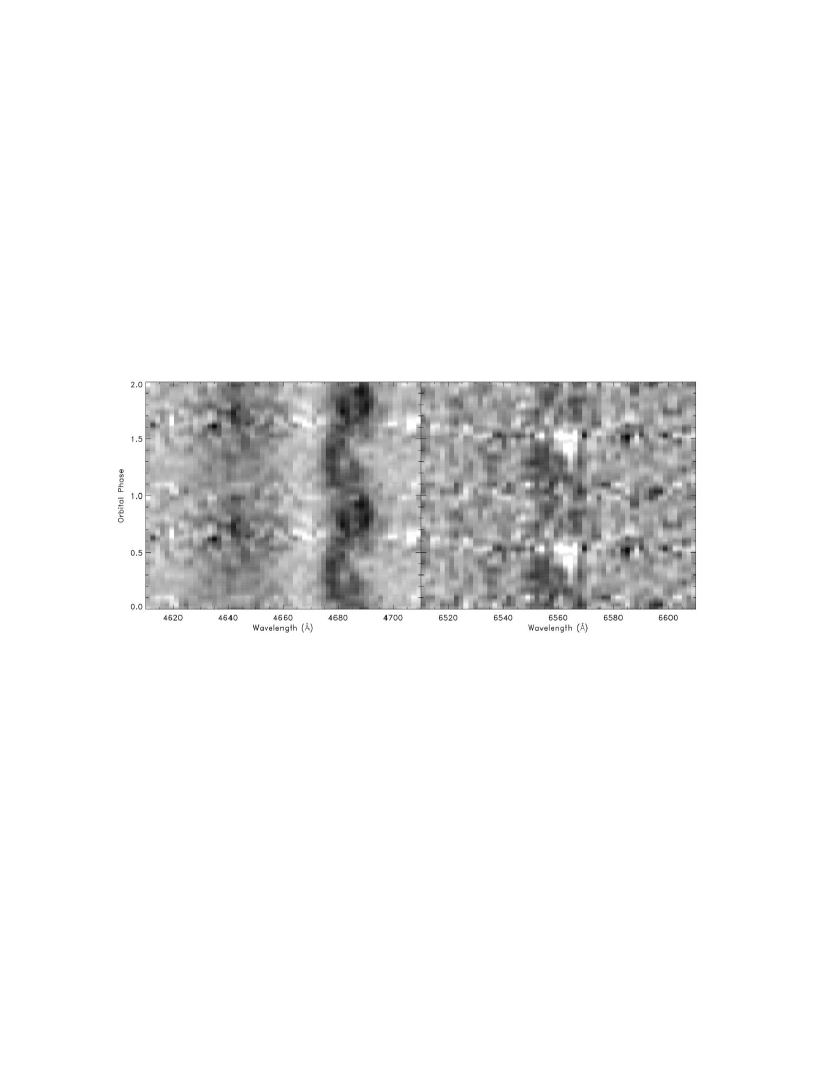
Figure 6: Trailed spectrograms of XTE J2123–058. Data have been phase-binned, with the same data plotted twice. The left hand panel shows behaviour of C iii/N iii 4640 Å and He ii 4686 Å emission. The right hand panel shows blended He ii 6560 Å and H$\alpha$ behaviour. Note the phase 0.5 H$\alpha$ absorption component; the white spot in the right hand panel.

The Bowen blend light curve appears similar to the continuum light curves shown in Fig. 3. Bowen emission may therefore originate on the heated face of the companion star, with the modulation arising from the varying visibility of the heated region.

He ii light curves show a double peaked structure with a strong peak near phase 0.75 and a weaker one near 0.25. We should be cautious in interpreting this light curve in detail, however, as the complex line behaviour seen in the trailed spectrogram indicates multiple emission sites; the integrated light curve is an average of different light curves of several regions.

H$\alpha$ emission is blended with He ii 6560 Å, and as discussed in Sect. 4 also comprises several components. The most striking is the transient absorption component seen near phase 0.5. This can be clearly seen in the light curve and the trailed spectrogram. The light curve is deceptive as it also reflects changes in the emission flux; it suggests that the absorption feature is centred at phase 0.5, but, as can be seen from the trailed spectrogram, this is not really the case. The feature begins quite sharp and red, around phase 0.3 and then becomes progressively more extended to the blue, fading out by phase 0.6. Whilst it is sometimes difficult to distinguish an absorption component from an absence of emission, that is not a problem here; the absorption definitely extends below the continuum as can clearly be seen in Fig. 7.

Figure 7: Average spectra near H$\alpha$ (lower) together with average of phases 0.35–0.55 alone (upper). Real absorption can clearly be seen in the upper spectrum.

6 Doppler tomography

We have used the technique of maximum entropy Doppler tomography (Marsh & Horne 1988) to identify He ii 4686 Å emission sites in velocity space. Our results are shown in Fig. 8. The analytical back-projection method gave similar results. We should beware, however, that one of the fundamental assumptions of Doppler tomography, that we always see all of the line flux at some velocity, is clearly violated, as the integrated line flux is not constant. We attempt to account for this by normalising the spectra (dividing by a smooth fit to the He ii 4686 Å light curve in Fig. 5). If we do not normalise then the structure of the derived tomogram is very similar, so our results do not appear to be sensitive to this difficulty.

Ideally, to perform Doppler tomography we should know the systemic velocity of the binary. We have no a priori knowledge of this, so we estimate it from the He ii 4686 Å line itself. This is done by repeating the tomographic analysis for different assumed mean velocities and seeking to minimise the residuals of the fit of the reconstructed spectrogram to the data (Marsh & Horne 1988). Our measured heliocentric systemic velocity is $\sim-90$ km s^-1 The implications of this velocity are discussed in Sect. 7.6.

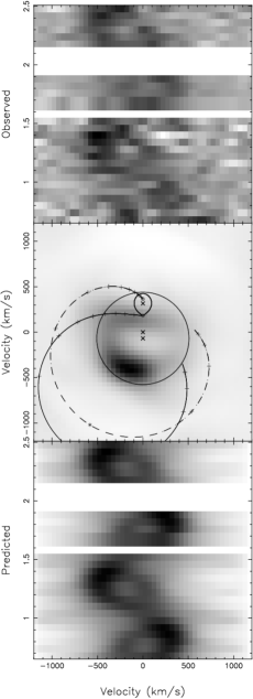
Figure 8: Doppler tomogram of He ii 4686 Å emission in XTE J2123–058. The upper panel shows the observed trailed spectra, normalised to constant total line flux. The middle panel shows the tomogram itself, and the lower panel shows the ideal trailed spectrogram reconstructed from the tomogram. In the middle panel, the solid arc is the ballistic stream trajectory, the dashed arc the Keplerian (disc) velocity at the stream position and the large circle is the Keplerian velocity at the outer disc edge. Phases below 1.6 come from the first night, those above this from the second; three complete cycles have been omitted for clarity.

In order to interpret the tomogram quantitatively, we also require estimates of system parameters. These were derived from results of fits to outburst light curves (see Paper I). The parameters we assume are given in Table 3. The masses deserve comment. The light curve fits only provide a significant constraint on the mass ratio, of $q=M_{1}/M_{2}=4.6^{+0.5}_{-0.2}$. To obtain actual masses, one must make physical assumptions. We assume that the neutron star has a typical mass of $M_{1}\sim 1.4$ M_☉ (see Thorsett & Chakrabarty 1999 for a review of neutron star masses) and hence that the companion should have a mass of 0.3 M_☉. As discussed in Paper I, a main sequence companion should have a mass of 0.6 M_☉ so it is likely that the companion is evolved and undermassive. Other SXTs do appear to have undermassive companions (Smith & Dhillon 1998), so this is a very plausible scenario, and one which is consistent with theoretical predictions (King, Kolb & Burderi 1996) that short period neutron star LMXBs should only be transient if they have evolved companions.

Table 3: Adopted system parameters. These are taken from Paper I except where discussed in the text.

$P_{\rm orb}$	0.24821 d
$i$	73∘
$M_{1}$	1.4 M☉
$M_{2}$	0.3 M☉
$R_{\rm L_{1}}$	$6.6\times 10^{10}$ cm
$R_{\rm disc}$	0.75 $R_{\rm L_{1}}$

The dominant emission site (corresponding to the main S-wave) appears on the opposite side of the neutron star from the companion. For any system parameters, it is inconsistent with the heated face of the companion and the stream/disc impact point. There is a fainter spot near the $\rm L_{1}$ point, corresponding to the fainter S-wave, which is possibly associated with the accretion stream. There also appears to be a loop connecting these two spots and a fainter arc on the right completing the circle. As noted above, however, the assumption that all the line flux is always visible at some velocity is not true for these data, and normalising the total flux is only an approximate solution when several emission components are present. It is likely, therefore, that some low-level artefacts are present and so weaker features in the tomogram may not represent real emission sites. To test this, we have also generated tomograms in which data along the S-wave corresponding to the bright spot are given a very low weight (see Steeghs et al. 2000). This should prevent artefacts due to misfitting of the time-dependence of this feature. We find that the upper left loop appears robustly, and is likely to be a real structure. The apparent arc completing the circle on the right does not appear and so is probably spurious. It is notable that nearly all emission has a lower velocity than Keplerian material at the outer disc edge could have, and so if associated with the disc requires sub-Keplerian emission.

7 Discussion

7.1 A neutron star SW Sex system?

In several respects XTE J2123–058 resembles the SW Sex class of cataclysmic variables. These are all novalike variables, typically seen at a relatively high inclination. Their main defining characteristics are (Thorstensen et al. 1991; Horne 1999; Hellier 2000):

1. Balmer lines are single-peaked and their motions lag behind that of the white dwarf. In a Doppler map emission is typically (though not always) concentrated in the lower-left quadrant at velocities lower than any part of the disc. A high velocity component is detectable with velocity semi-amplitude $\sim 1000$ km s^-1. This has the same phasing as the low velocity component; and their separate identity is vigorously debated.

2. Transient absorption lines are seen. These are strongest near phase 0.5 or slightly earlier and move from red to blue between phases 0.2 and 0.6.

3. Continuum eclipses have a V-shaped profile implying a flatter temperature distribution than expected theoretically. Balmer line eclipses are shallow and occur earlier than continuum eclipses. Red shifted emission remains visible at mid-eclipse.

On the first two points XTE J2123–058 shows striking similarities to the SW Sex systems. Anomalous emission line behaviour is most clearly seen in He ii 4686 Å in this higher excitation system. This line appears, on average, single peaked. The emission is concentrated in the lower-left quadrant at sub-Keplerian velocities. A high velocity component is not detected, but cannot be ruled out without higher quality data. Transient absorption is seen in the Balmer lines before and around phase 0.5. It begins slightly redshifted and moves to the blue. XTE J2123–058 is the SXT with the highest known inclination ($i=73^{\circ}\pm 4^{\circ}$; Paper I), strengthening the similarity to SW Sex systems. It does not deeply eclipse, however, so it is impossible to comment on the third point.

Various models have been proposed for the SW Sex phenomenon including bipolar winds, magnetic accretion and variations on a stream overflow theme. Current opinion favours the latter interpretation, with the stream either being accelerated out of the Roche lobe by a magnetic propeller, or re-impacting the disc. Both of these models are discussed in more detail below.

7.2 Is this behaviour typical of LMXBs?

The only other SXT for which outburst Doppler tomography of adequate quality is available is the black hole candidate GRO J0422+32 (Casares et al. 1995). Using ephemerides determined subsequently (Harlaftis et al. 1999), emission in this object appears to originate from the accretion stream/disc impact point. These data were obtained in the December 1993 mini-outburst, $\sim 500$ d after the peak of the primary outburst.

Amongst other short-period neutron star LMXBs in an active state, only 2A 1822–371 (Harlaftis, Charles & Horne 1997) has Doppler tomography. This was observed in H$\alpha$ and exhibited disc emission enhanced towards the stream impact point. Similar behaviour is suggested by a radial velocity analysis of He ii (Cowley, Crampton & Hutchings 1982). This is different to what we see in XTE J2123–058. Radial velocity analyses of other systems, however, suggest similar behaviour to that seen here. 4U 2129+47 shows a very similar blue spectrum to XTE J2123–058 (Thorstensen & Charles 1982). Clear variations in the He ii 4686 Å radial velocity are seen with maximum radial velocity around phase 0.7–0.8 and semi-amplitude $216\pm 70$ km s^-1. Spectroscopy of EXO 0748–676 (Crampton et al. 1986) also reveals radial velocity modulations in the He ii 4686 Å line. The radial velocity curve measured from the line base shows maximum velocity at phase $0.76\pm 0.16$ with semi-amplitude $210\pm 92$ km s^-1. For comparison, a similar radial velocity curve fit to our He ii spectra (Hynes et al. 1998) yielded maximum velocity close to phase 0.75 with semi-amplitude $\sim 180$ km s^-1. Augusteijn et al. (1998) studied 4U 1636–536 and 4U 1735–44 and found the two systems similar to each other. Both show He ii modulations with semi-amplitude 140–190 km s^-1 with maximum radial velocities measured at phases 0.87–1.04. We therefore suggest that the behaviour we see is common, but not universal, in short period neutron star LMXBs in a high state.

7.3 The magnetic propeller interpretation

It is possible to explain the behaviour of the He ii 4686 Å line in terms of the magnetic propeller model. This model also provides a possible mechanism for explaining the transient Balmer absorption, although this is less satisfactory.

The essence of this model is that in the presence of a rapidly rotating magnetic field, accreting diamagnetic material may be accelerated tangentially, leading to it being ejected from the system. It is easy to see how such a scenario may arise due to a rapidly spinning, magnetised compact object. This mechanism has been invoked to explain the unusual behaviour of the cataclysmic variable AE Aqr in terms of a magnetic field anchored to a spinning white dwarf (Wynn, King & Horne 1997; Eracleous & Horne 1996). It is also likely that magnetic propellers driven by neutron star magnetic fields exist, as proposed by Illarianov & Sunyaev (1975). These may be very important in suppressing accretion in neutron star SXTs in quiescence; see Menou et al. (1999) and references therein for a discussion of this situation. There is an important difference of scale, however; spin periods of white dwarfs are $\ga 30$ s; spin periods of neutron stars are typically of order milliseconds. For XTE J2123–058, $P_{\rm spin}=3.92\pm 0.22$ ms was suggested by Tomsick et al. (1999) based on the beat-frequency model for kilohertz QPOs. This identifies the separation of the QPO peaks with the spin period. While the peak separation is not always exactly constant, Psaltis et al. (1999) examine the model and conclude that the separation is still likely to be close to the spin period. Thus the spin period of the neutron star in XTE J2123–058 is probably not far from 4 ms. For such rapid rotation we must consider the light-cylinder, defined by the radius at which the magnetic field must rotate at the speed of light to remain synchronised with the compact object spin. Outside of this radius, the magnetic field will be unable to keep up and hence becomes wound up. This will make the propeller less effective, although it may still produce some acceleration (Wynn et al. 1997; Wynn priv. comm.). For a $\sim 4$ ms spin period in XTE J2123–058, this is $\sim 6\times 10^{-5}\,R_{\rm disc}$; for comparison, the closest approach of a ballistic stream is $\sim 0.2\,R_{\rm disc}$. We would therefore not expect a neutron star propeller to strongly affect the stream overflow material, although simulations are needed to test this. An alternative mechansim was suggested by Horne (1999) for SW Sex systems, in which a magnetic propeller can arise from the magnetic fields of the disc itself. This has problems, in that it should very efficiently remove angular momentum from the disc (Wynn & King priv. comm.), but this could perhaps be overcome if only a small fraction of stream material passes through the propeller. This mechanism allows much lower angular velocities for the field and may be the only large scale propeller mechanism possible in a neutron star system.

We adopt the parameterisation used by Wynn, King & Horne (1997) to describe the magnetic propeller in AE Aqr. The magnetic field is simplistically modelled as a dipole with angular velocity $\omega_{\rm f}$. While such a field may be a reasonable representation of that of a compact star (white dwarf or neutron star), it is clearly a gross simplification of that of a disc-anchored propeller. In the latter case the net effect would probably arise from a mixture of unstable field structures of varying strengths and anchored at a range of radii. For simplicity and consistency with existing work on magnetic propellers, however, we approximate the complex field structure with a single rotating dipole. The propeller mechanism assumes that the flow breaks up into diamagnetic blobs of varying size and density. The field can only partially penetrate the blobs, and hence they are accelerated, but not locked to the field lines. The magnetic acceleration on a blob is given by $g_{\rm mag}=-k[v-v_{\rm f}]_{\perp}$, where $v$ is the stream velocity, $v_{\rm f}=r\omega_{\rm f}$ is the field velocity and the component of the velocity difference perpendicular to the field is taken. The parameter $k$ parameterises our ignorance of the magnetic field strength and blob size and density, and following Wynn & King (1995) we adopt the functional dependence $k=k_{0}(r/r_{0})^{-2}$, where $r_{0}=10^{10}$ cm. Different blob sizes and densities will lead to a spread of values of $k_{0}$ and hence different trajectories. The uncertainty in the angular velocity of the magnetic field is also factored into the uncertainty in $k_{0}$ provided it is high enough that $v_{\rm f}\gg v$ at all points along the stream trajectory, and low enough that all regions of interest are within the light cylinder. For XTE J2123–058, this corresponds to a field period of approximately $500\,{\rm s}\gg P_{\rm spin}\gg 10$ s (i.e. a field anchored at $0.16r_{\rm disc}\gg R\gg 0.012r_{\rm disc}$). Within this regime varying $P_{\rm spin}$ has the same effect as varying $k_{0}$, and different trajectories can be described by a single parameter. This gives a plausible range of radii for anchoring the magnetic field and so we adopt this simple case for our model and arbitarily set $P_{\rm spin}=50$ s, corresponding to a field anchored at radius $\sim 0.03$ of the disk radius. As noted above, this is only an approximation to a more chaotic field structure.

As we are considering a system in which most of the accretion likely proceeds through the disc, we assume that the propeller mechanism acts only on overspill from the stream-disc impact point. Our model therefore calculates a trajectory which is purely ballistic until it reaches the disc edge and is subject to a propeller force thereafter. Quantitatively, this makes little difference to the results compared to allowing the magnetic force to act everywhere on the stream.

We adjust the $k_{0}$ parameter to find a trajectory which passes through the central emission on the tomogram. This is shown in Fig. 9 together with two bracketting trajectories to show the dependence on $k_{0}$. For this to be a plausible model, we also require an explanation for why one particular place on the trajectory is bright. Such an explanation is offered by Horne (1999): there is a point outside the binary at which trajectories for different values of $k$ intersect. At this point, faster moving blobs cross the path of slower blobs and enhanced emission might be expected. This can be seen in Fig. 9. We identify the region where the trajectories collide with the emission region.

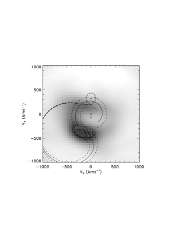
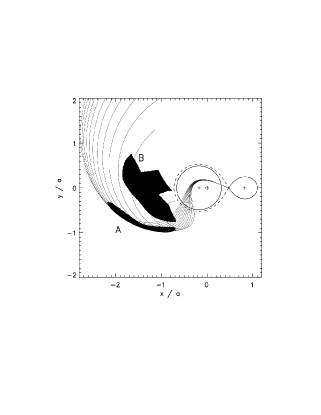
Figure 9: A magnetic propeller model for He ii emission; see text for details of the model. The left hand panel shows the tomogram with three model trajectories corresponding to different values of $k_{0}$. The white shading indicates the region of strongest emission. In the right hand panel, the trajectories are shown in real space in the corotating frame; units are the binary separation. Phase 0.0 corresponds to viewing from the right of the diagram, with 0.25 from the bottom, 0.5 from the left and 0.75 from the top. The region of strongest emission in the tomogram maps to the solid area A, assuming the propeller velocity field. It is striking that this emission is coincident with the location where the stream trajectories intersect in real space. Points within solid area B will obscure the disc with the phasing and velocity observed in H$\alpha$.

To make a quantitative comparison of our data with the model, we transform the brightest emission spot of the tomogram into real space. Such a conversion is not in general possible, of course, but can be performed if system parameters and a velocity field are assumed, provided that the velocity–space mapping is one–one or many–one. That is true in this case if we only consider emission from the first loop around the binary. We construct a series of trajectories in velocity space defined by uniform steps in $k_{0}$, and select points for which the tomogram intensity is above a certain value. The selected points are shown spatially in the right hand panel of Fig. 9 as region A. We can see that, subject to the assumptions made, emission does occur at the point where trajectories cross. Our data are therefore consistent with the emission mechanism suggested by Horne (1999). We emphasise that this spatial map is only valid in the context of the propeller model.

One point should be noted. Hellier (2000) suggests that the propeller model should predict a continuous S-wave, which is not seen. This is not necessarily the case. If the region in which accelerated blobs collide is optically thick in the line then emission is expected predominantly from the inner edge of this region where fast moving blobs impact slow moving blobs. For the geometry we have considered, as can be seen in Fig. 9, this will result in emission predominantly towards the top of the figure. This corresponds to seeing maximum emission near phase 0.75, exactly as is observed in our data and in that of SW Sex systems, such as PX And (Hellier & Robinson 1994). The phase dependence of emission line flux is therefore not a problem with the propeller model, but instead a prediction made by it.

We have demonstrated that both our He ii tomogram and the line-flux light curve are consistent with emission from the region where material ejected by a propeller is expected to converge. Can we interpret the phase-dependent Balmer absorption as arising from the same region, as was suggested by Horne (1999) in the context of SW Sex systems? This model certainly predicts some ejecta in front of the disc and/or companion at phases 0.3–0.6 where absorption is observed. As can be seen in Fig. 6, however, we also have information on the absorption kinematics. We can thus perform a similar mapping to that used for the emission to determine if absorption is predicted with the right phasing and kinematics and where it would have to originate. We construct a fine grid of trajectories and for each point calculate the phase and velocity at which this would pass in front of the centre of the disc. If this lies within the absorption region in the trailed spectrogram then we mark that point as within region B in Fig. 9. We find that the resulting points do populate the observed absorption region fully, so the model can produce the absorption. The material involved, however, is not on the same trajectories as the emission, but occurs on lower velocity tracks. The absence of emission from region B may indicate that only high velocity material undergoes sufficiently energetic collisions to produce He ii emission. The converse, that absorption does not reach to region A, could arise because the emission region has a higher brightness temperature in the lines than the disc continuum. It also remains unexplained why absorption is only seen along part of the trajectories. For the low velocity trajectories, some material may fall back onto the disc. The phase dependence may also be related to the height of the absorbing material above the disc plane, as may the lack of absorption from region A. Clearly these are further questions to address in developing a full propeller model for these data. Such a three-dimensional treatment is beyond the scope of our simplistic model however, and we leave these points as observational requirements that a full model must satisfy.

7.4 The stream overflow and disc re-impact interpretation

The most popular alternative explanation for the SW Sex phenomenon is the accretion stream overflow and re-impact model. This was originally suggested by Shafter, Hessman & Zhang (1988); for a recent exposition see Hellier (2000).

In this model the overflowing stream can be thought of in two regions. The initial part of the stream produces the transient absorption when seen against the brighter background of the disc. The latter part, where the overflow re-impacts the disc, is seen in emission giving rise to the high velocity component. To reproduce observations, this model requires a number of refinements.

In the simplest form of the model, the overflow stream should produce absorption at all phases; it always obscures some of the disc. This problem is overcome by invoking a strongly flared disc so that the overflow stream is only visible near phase 0.5. We see an absorption depth of 15 per cent of the continuum flux. At this phase, at least 40  per cent of the continuum flux actually comes from the companion star, so we require absorption of 25 per cent of the visible disc light to achieve the observed depth, and hence at least 25 per cent of the visible disc to be covered by the obscuring material; more if absorption is not total. With a strongly flared disc, however, the near side may be self-occulted so only $\sim 10$ per cent of the total disc area need be covered by the overflowing material. This is not implausible, and simulations can produce such a messy splash (Armitage & Livio 1998). There are difficulties in invoking a strongly flared disc in XTE J2123–058, however. It has lower inclination than typical SW Sex systems: $73^{\circ}\pm 4^{\circ}$ (Paper I) and does not show X-ray eclipses. The strong photometric modulation due to heating of the companion also constrains the amount that the disc can be flared; too much and the companion will be shielded from X-rays. In Paper I an upper limit to the flare angle of $8\aas@@fstack{\circ}6$ was derived (99 per cent confidence) from fitting of optical lightcurves $\sim 10$ days after the WHT observations. Comparing this with the viewing angle of $17^{\circ}\pm 4^{\circ}$ it is clear that the near side of the disc, and hence the overflowing material, should never be completely obscured, rendering the phase dependence difficult to account for.

The re-impact model requires that the strong emission in the lower-left quadrant be produced by overlap of weaker emission from the high-velocity component (the re-impact point) and the disc. To produce emission at the low velocities observed, however, requires the ‘disc’ component to be sub-Keplerian by a significant amount. This problem is not peculiar to XTE J2123–058, for which parameters are uncertain, but common to the SW Sex class in general. In our case, such a sub-Keplerian ring may be present, but it is likely that this is not a real feature. There is no evidence for a high velocity component, but given our data quality, this is also inconclusive.

7.5 X-ray signatures of the absorbing material

In principal X-ray observations can provide a diagnostic tool not available in SW Sex systems, and could constrain the location of the absorbing material. In the overflow and reimpact model it is necessary for the disc to be highly flared to reproduce the phase dependence of the absorption, and for the overflow to splash over a moderately large area to reproduce the absorption depth. One might then expect that some of the overflowing material would cross our line of sight to the neutron star and produce X-ray dips in the phase range $\sim 0.6$–1.0, as seen in other high inclination LMXBs, the dipping sources. Such dips are also possible in the propeller model, although not necessary as this does not require a flared disc or extended splash. This model would, however, be expected to produce X-ray dips in the same range as the transient H$\alpha$ absorption, $\sim 0.3$–0.6.

Tomsick et al. (1998b) reported no evidence for an X-ray orbital modulation in RXTE/PCA data. We have obtained archival PCA data from 1998 July 14 and 22 and examined Standard-2 mode lightcurves to reexamine this issue. Background subtraction was done using bright source background models dated 1999 September 17 and lightcurves were extracted for both the whole PCA bandpass and for 3–5 keV only. We find no evidence for dips of longer than 16 s with depth greater than 10 per cent at any orbital phase. We have also phase-binned all of these data to search for broader structures. Approximately 60 per cent of phase bins have data combined from at least two binary orbits; amongst these, with the exception of the X-ray bursts (Takeshima & Strohmayer 1998; Tomsick et al. 1998b) there are no excursions of greater than $\pm 10$ per cent about the mean.

It is unfortunate that the RXTE data is not simultaneous with our WHT observations and phase coverage is incomplete. Thus we can say that X-ray observations provide no evidence in favour of either the reimpact or propeller models, but they do not rule either out.

7.6 The origin of XTE J2123–058

The question of the origin of XTE J2123–058 was raised in Sect. 1: is it intrinsically a halo object or was it kicked out of the Galactic plane? The strongest evidence is provided by the ratio of N iii/C iii-He ii. This is typical of Galactic LMXBs and is inconsistent with known halo objects. In principal, the systemic velocity is also an important clue. For this object to have reached its present location it must have received a kick when the neutron star was formed, and hence it may now have a large peculiar velocity (150–400 km s^-1, Homan et al. 1999). Our measured radial component of velocity is $\sim-90$ km s^-1 which is not inconsistent with the predictions of Homan et al., which could also be lowered if the source distance is less than the 10 kpc value assumed by those authors. We should add a note of caution, however, as systemic velocities inferred from emission lines are sometimes unreliable; a definitive measurement of the systemic velocity must await a study based on photospheric absorption lines of the companion star.

8 Conclusions

Three key issues were raised in Sect. 1 and we conclude by returning to these. As a neutron star transient, XTE J2123–058 is valuable for comparison with black hole systems. Of the latter, GRO J0422+32 is the most similar, and appears to show a less steep optical spectral energy distribution than XTE J2123–058, consistent with the suggestion of King et al. (1997) that irradiation is more efficient in neutron star systems. The high orbital inclination of XTE J2123–058 has made possible Doppler tomography of He ii emission, and the detection of transient Balmer line absorption. These effects suggest similarities to SW Sex type cataclysmic variables. Unlike SW Sex systems, XTE J2123–058 shows characteristic SW Sex emission line kinematic effects (in He ii) decoupled from transient absorption providing constraints not possible when both effects occur in the same line. We have examined our results in the context of stream overflow models applied to these systems, both with stream reimpact and propeller ejection. The reimpact model, while plausible physically, has difficulties accounting for our observations. The propeller model can successfully explain both emission and absorption behaviour, but has yet to overcome theoretical difficulties. Both theoretical work, and higher quality observations will be required to conclusively decide between the models, and it remains possible that neither is correct. As an object currently located in the Galactic halo, the origin of XTE J2123–058 is also of interest. Bowen line strengths, relative to He ii, indicate abundances similar to Galactic sources but different to globular cluster and Magellanic LMXBs and hence we suggest that this object was formed in the plane and subsequently kicked out.

References

- [Armitage & Livio 1998] Armitage P. J., Livio M., 1998, ApJ, 493, 898
- [Augusteijn et al. 1998] Augusteijn T., van der Hooft F., de Jong J. A., van Kerkwijk M. H., van Paradijs J., 1998, A&A, 332, 561
- [Callanan et al. 1995] Callanan P. J, et al., 1995, ApJ, 441, 786
- [Casares et al. 1995] Casares J., Marsh T. R., Charles P. A., Martin A. C., Martin E. L., Harlaftis E. T., Pavlenko E. P., Wagner R. M., 1995, MNRAS, 274, 565
- [Casares et al. 1998] Casares J., Serra-Ricart M., Zurita C., Gomez A., Alcalde D., Charles P., 1998, IAU Circ. 6971
- [Cowley, Crampton & Hutchings 1982] Cowley A. P., Crampton D., Hutchings J. B., 1982, ApJ, 255, 596
- [Crampton et al. 1998] Crampton D., Cowley A. P., Stauffer J., Ianna P., Hutchings J. B., 1986, ApJ, 306, 599
- [Eracleous & Horne 1996] Eracleous M., Horne K., 1996, ApJ, 471, 427
- [Harlaftis, Charles & Horne 1997] Harlaftis E. T., Charles P. A., Horne K., 1997, MNRAS, 285, 673
- [Harlaftis et al. 1999] Harlaftis E., Collier S., Horne K., Filippenko A. V., 1999, A&A, 341, 491
- [Hellier 2000] Hellier C., 2000, in proc. Warner Symposium on Cataclysmic Variables, eds. P. A. Charles, A. R. King, D. O’Donoghue, New Astronomy Reviews, 44, 131
- [Hellier & Robinson 1994] Hellier C., Robinson E. L., 1994, ApJ, 431, L107
- [Homan et al. 1998] Homan J., van der Klis M., van Paradijs J., Mendez M., 1998, IAU Circ. 6971
- [Homan et al. 1999] Homan J., Méndez M., Wijnands R., van der Klis M., van Paradijs J., 1999, ApJ, 513, L119
- [Horne 1999] Horne K, 1999, in Magnetic Cataclysmic Variables, eds. K. Mukai, C. Hellier, ASP, p. 349
- [Hynes & Haswell 1999] Hynes R. I., Haswell C. A., 1999, MNRAS, 303, 101
- [Hynes et al. 1998] Hynes R. I., Charles P. A., Haswell C. A., Casares J., Serra-Ricart M., Zurita C., 1998, IAU Circ. 6976
- [Illarionov & Sunyaev 1975] Illarionov A. F., Sunyaev R. A., 1975, A&A, 39, 185
- [Ilovaisky & Chevalier 1998] Ilovaiksy S. A., Chevalier C., 1998, IAU Circ. 6975
- [King 1985] King D. L., 1985, RGO/La Palma Technical Note 31
- [King, Kolb & Burderi 1996] King A. R., Kolb U., Burderi, L., 1996, ApJ, 464, L127
- [King & Kolb 1997] King A. R., Kolb U., 1997, ApJ, 481, 918
- [King, Kolb & Szuszkiewicz 1997] King A. R., Kolb U., Szuszkiewicz E., 1997, ApJ, 488, 89
- [Krelowski et al. 1987] Krelowski J., Walker G. A. H., Grieve G. R., Hill G. M., 1987, ApJ, 316, 449
- [Levine, Swank & Smith 1998] Levine A., Swank J., Smith E., 1998, IAU Circ. 6955
- [Marsh & Horne 1988] Marsh T. R., Horne K., 1988, MNRAS, 235, 269
- [Menou et al. 1999] Menou K., Esin A. A., Narayan R., Garcia M. R., Lasota J. -P., McClintock J. E., 1999, ApJ, 520, 276
- [Motch & Pakull 1989] Motch C., Pakull M. W., 1989, A&A, 214, L1
- [Munari & Zwitter 1997] Munari U., Zwitter T., 1997, A&A, 318, 274
- [Oke 1990] Oke J. B., 1990, AJ, 99, 1621
- [Psaltis et al. 1998] Psaltis D. et al., 1998, 501, L95
- [Schlegel, Finkbeiner & Davis 1998] Schlegel D. J., Finkbeiner D. P., Davis M., 1998, ApJ, 500, 525
- [Shafter, Hessman & Zhang 1988] Shafter A. W., Hessman F. V., Zhang E. H., 1988, ApJ, 327, 248
- [Shrader et al. 1994] Shrader C. R., Wagner R. M., Hjellming R. M., Han X. H., Starrfield S. G., 1994, ApJ, 327, 248
- [Smith & Dhillon 1994] Smith D. A., Dhillon V. S., 1998, MNRAS, 301, 767
- [Soria et al. 1999] Soria R., Wu K., Galloway D., 1999, MNRAS, 309, 528
- [Steeghs 2000] Steeghs D. et al., 2000, in preparation
- [Takeshima & Strohmayer 1998] Takeshima T., Strohmayer T. E., 1998, IAU Circ. 6958
- [Thorsett & Chakrabarty 1999] Thorsett S. E., Chakrabarty D., 1999, ApJ, 512, 288
- [Thorstensen & Charles 1982] Thorstensen J. R., Charles P. A., 1982, ApJ, 253, 756
- [Thorstensen et al. 1991] Thorstensen J. R., Ringwald F. A., Wade R. A., Schmidt G. D., Norsworthy J. E., 1991, ApJ, 102, 272
- [Tomsick et al. 1998a] Tomsick J. A., Halpern J. P., Leighly K. M., Perlman E., 1998a, IAU Circ. 6957
- [Tomsick et al. 1998b] Tomsick J. A., Kemp J., Halpern J. P., Hurley-Keller D., 1998b, IAU Circ. 6972
- [Tomsick et al. 1998b] Tomsick J. A., Halpern J. P., Kemp J., Kaaret P., 1999, ApJ, 521, 341
- [van der Klis 1999] van der Klis M., 1999, in proc. 3rd William Fairbank Meeting, Rome, 1998 June 29 – July 4 (astro-ph/9812395)
- [van Paradijs & White 1995] van Paradijs J., White N., 1995, ApJ, 447, L33
- [Wynn & King & 1995] Wynn G. A., King A. R., 1995, MNRAS, 275, 9
- [Wynn, King & Horne1997] Wynn G. A., King A. R., Horne K., 1997, MNRAS, 286, 436
- [Zurita & Casares 1998] Zurita C., Casares J., 1998, IAU Circ. 7000
- [Zurita, Casares & Hynes 1998] Zurita C., Casares J., Hynes R. I., 1998, IAU Circ. 6993
- [Zurita et al. 2000] Zurita C. et al., 2000, MNRAS, 316, 137