Studying the Galactic Bulge Through Spectroscopy of Microlensed Sources:
II. Observations

Abstract

The spectroscopy of microlensed sources towards the Galactic bulge provides a unique opportunity to study (i) the kinematics of the Galactic bulge, particularly its far-side, (ii) the effects of extinction on the microlensed sources, and (iii) the contributions of the bulge and the disk lenses to the microlensing optical depth. We present the results from such a spectroscopic study of 17 microlensed sources carried out using the ESO Faint Object Spectrograph (EFOSC) at the 3.6 m European Southern Observatory (ESO) telescope. The spectra of the unlensed sources and Kurucz model spectra were used as templates to derive the radial velocities and the extinctions of the microlensed sources. It is shown that there is an extinction shift between the microlensed population and the non-microlensed population but there is no apparent correlation between the extinction and the radial velocity. This extinction offset, in our best model, would imply that 65% of the events are caused by self-lensing within the bulge. The sample needs to be increased to about 100 sources to get a clear picture of the kinematics of the bulge.

1 INTRODUCTION

By now, several authors (Kiraga & Paczyński, 1994; Paczyński et al., 1994b; Mollerach & Roulet, 1996; Zhao et al., 1995) have pointed out that the stars within the Galactic bulge may play a dominant role as gravitational lenses, and a significant fraction of the detected events may be due to lensing by stars within the bulge. If a significant fraction of these events are indeed due to lenses within the bulge, then the microlensing characteristics can provide a powerful technique of deriving the stellar mass density and mass function within the Galactic bulge (Zhao et al., 1995). However, the contributions of different populations to the microlensing optical depth remain uncertain, and their determination is important in using the microlensing characteristics to derive other quantities such as the stellar mass density and the stellar mass function.

If the lensing is caused predominantly by bulge stars, then a major fraction of the lensed stars will be at the far side of the bulge so that there are enough stars in front to cause the lensing. Thus they would be fainter in general, and it was shown by Stanek (1995) that the magnitude offset between the lensed sources and non-lensed sources can be a good measure of the fraction of the events caused by bulge lenses. A similar test was suggested by Kane & Sahu (2000) (hereafter referred to as paper I) through the measurement of extinction and it was shown that an extinction offset may be measurable from the spectra of lensed and non-lensed sources. This test used the principle that the lensed stars should have larger extinction since they would predominantly be on the far side.

If the sources are predominantly in the far side of the bulge, then the spectra of these sources give a unique opportunity to derive the radial velocities of the objects in the far side of the Galactic bulge. The radial velocities derived from the observed spectra can be combined with the proper motion derived from the microlensing time scales to determine the 3-dimensional velocity structure of the far side of the Galactic bulge.

This paper presents the results of a spectroscopic study of microlensed sources conducted using data obtained with the 3.6 m telescope of the European Southern Observatory (ESO) at La Silla, Chile. Kurucz model spectra were used to create theoretical extinction effects for various spectral classes of stars towards the Galactic bulge. These extinction effects are used to interpret spectroscopic data consisting of a sample of microlensed stars towards the Galactic bulge. The extinction offsets of the lensed source with respect to the average population is derived and a measurement of the fraction of bulge-bulge lensing is made. Measurements of the radial velocities of these sources are used as an attempt to determine the kinematic properties of the far side of the Galactic bulge.

2 OBSERVATIONS AND DATA REDUCTION

2.1 Details of the Observations

The observations were taken with the ESO 3.6 m telescope using the ESO Faint Object Spectrograph and Camera (EFOSC). The data were obtained in two observing runs: the first run was from June 28 to July 1, 1995 during which a major part of the observations were taken, and the second run was on the night of June 14, 1996 during which only one source was observed. The sky condition was clear during the whole 1995 observing run; the 1996 observations, however, were affected by passing cirrus and clouds. Table 1 shows the grisms that were used for the observations. The CCD detector used has $512\times 512$ pixels and a pixel scale of 0.61 arcsec pixel^-1 both in the dispersion and the cross-dispersion directions. The seeing during the observations was $\sim$1 arcsec, and a slit-width of $1.5^{\prime\prime}$ was used for all the observations. The spectral resolution depends on the chosen slit width, and for our observations, the true spectral resolution is approximately 2.46 times the dispersion (Å per pixel) shown in Table 1. At the time of observations, the camera was set to have a gain of 3.8 electrons per count for which the read-out noise is 8.5 electrons per pixel.

As the name implies, the EFOSC is both an imaging and a spectrographic camera. The imaging capability of this spectrograph greatly facilitates the spectroscopic observations of stars in crowded fields such as the Galactic bulge by examining the field first, before placing the slit on the object of interest. This facility was particularly useful for our purpose of simultaneously obtaining the spectra of a few non-microlensed sources along with the microlensed source, by placing them all along the same slit. In order to achieve this, an image was obtained first, with a typical integration time of about 2 minutes. This image was taken using a clear (unfiltered) aperture to avoid any shift while placing the slit. Then the slit was centered on the microlensed source and its orientation was set such that (i) it was close to the East-West direction (so that the differential atmospheric dispersion was minimum along the slit), and (ii) there were a sufficient number of non-lensed sources on the slit (which would be later used as the control sample in the analysis). Since the size of the detector is rather small ($512\times 512$ pixels), the spectral coverage in each setting is accordingly small. So it was generally necessary to take two separate spectra using two grisms in the blue and the red, in order to cover the wavelength range of our interest. This limited spectral coverage in a single grism setting had the advantage that the effect of the differential atmospheric dispersion at various wavelengths in a spectrum is minimal. Nevertheless, attempts were made to do the observations in low air-masses to further minimize any differential atmospheric dispersion at different wavelengths in a given setting.

To correct for the electronic noise associated with the detector readout, 5 bias exposures were taken every evening, the median of which was used for subtracting the bias level. To correct for pixel-to-pixel sensitivity variations of the detector, flat-field exposures were taken by observing a part of the dome illuminated with a tungsten lamp. Typically, 3 flat-field exposures were taken for each grism in the beginning of each night, the average of which was used during the data reduction.

For wavelength calibration, spectra were taken by illuminating the slit with a He lamp, followed by an Ar lamp in the same exposure. The combination of He and Ar was necessary to get enough lines both in the blue and the red region of the spectrum simultaneously. The rms deviation of the residuals from the dispersion relations for each grism are shown in Table 1. The lamp spectra were taken for each grism at the beginning and end of every night. The typical wavelength shift during a night was less than 0.1 pixels, which is not more than the rms deviation of the residuals from the dispersion relations.

Since this study is mostly interested in the relative fluxes and line strengths rather than their absolute values, observing a single standard star per night was deemed sufficient. The standard star LTT 9239 was used for the 1995 observations and the standard star LTT 8702 was used for the 1996 observations. The uncertainty in absolute flux calibration would normally be in the range of 10–20% in clear sky conditions and worse if the sky is not photometric, however the relative fluxes will be more accurate.

The spectra of 17 different microlensed sources were obtained during these observing runs. Since the purpose of this study is to compare the spectra of microlensed sources with a control sample of other stars, 5 non-lensed stars were chosen from each field whose spectra were also reduced. The microlensing events observed are summarized in Table 2, where $t_{E}$ is the time taken by the lens to cross the Einstein ring radius. This information has been extracted from the MACHO alerts (http://darkstar.astro.washington.edu/) and from the OGLE and DUO publications (Alard et al., 1995; Woźniak & Szymański, 1998). The binary events have an undetermined characteristic time scale $t_{E}$. The galactic longitude and latitude of the sources lie in the range $0.55\arcdeg<l<3.98\arcdeg$ and $-4.92\arcdeg<b<-2.68\arcdeg$ respectively. A summary of the observations of these events is shown in Table 3. DUO 95-BLG-2 and OGLE 95-BLG-3 were also observed, but the sky was scattered with clouds during these observations. As a result, the signal-to-noise in these spectra are considerably lower. Hence these two sources and their associated non-microlensed stars are not included in the following analysis.

2.2 Data Reduction

After the usual bias subtraction, the wavelength calibration for the entire 2-dimensional image was carried out through the lamp spectra obtained with the appropriate grism during that particular night. The 1-dimensional spectra were extracted for the microlensed source and 5 non-microlensed sources in the image using an extraction height of 5–7 pixels for each source. The images being crowded, sky subtraction was tricky, so care was taken in choosing an appropriate region for the sky subtraction. The spectra were corrected for atmospheric extinction using a model available for the ESO observing site (for details, see the MIDAS manual). The resulting 1-dimensional spectra were flux calibrated through a standard star observation carried out in the same night. The flat-field images obtained with the illuminated dome were found to be relatively smooth, and the pixel-to-pixel response variation was found to be small, so the flat-field images were not used in the reduction. Instead, the flat-fielding and the flux calibration was done through a single step through the standard star observations. These final 1-dimensional spectra are then used for further analysis.

3 ESTIMATING SPECTRAL TYPE, EXTINCTION, AND RADIAL VELOCITY

In order to process the large number of spectra that were obtained, a MIDAS script was written which estimates both the spectral type and the extinction for each individual spectrum. This script uses a large library of model spectra that was constructed from the Kurucz database and a cross-correlation technique to achieve this, as explained in more detail later. An additional script was written to determine the radial velocities of the microlensed and non-microlensed sources which uses a high signal-to-noise template spectrum and a cross-correlation technique. More details of the method used in these scripts are given in Section 3.2. (The script itself, with ample comments describing the algorithms, is published by Kane, (2000)).

3.1 The Model Spectra

The 1993 Kurucz stellar atmospheres atlas (Kurucz, 1993) covers a wide range of metallicities, effective temperatures, and gravities. The models were first developed by Kurucz in 1970 using the stellar atmosphere modeling program ATLAS (Kurucz, 1970). The 1993 atlas contains about 7600 models which are convenient to access using the IRAF (Image Reduction Analysis Facility) task synphot, which is available in the stsdas package developed at the Space Telescope Science Institute. The task synphot was used to extract a full grid of model spectra from the atlas, by specifying the appropriate range of temperatures, metallicities and the surface gravities, as explained below.

Figure 1: Surface gravity $\log g$ for luminosity classes I, III, and V.

To extract the model spectra from the atlas, an exhaustive list of stellar parameters was needed for each of the stellar sub-types and luminosity classes. The values for the effective temperature $T_{eff}$, the surface gravity $\log g$, and the absolute magnitude $M_{V}$ characterizing each star were obtained from Schmidt-Kaler’s compilation of physical parameters of stars (Schmidt-Kaler, 1982). However, the values of $\log g$ were found to be severely lacking in their coverage of the stellar sub-types and so the remaining values were determined from the interpolation of the values given by Schmidt-Kaler. As shown in Figure 1, a fourth-order polynomial of the form $y=ax^{4}+bx^{3}+cx^{2}+dx+e$ was fitted to the available data for each luminosity class. The coefficients for the polynomial fitted to each luminosity class are shown in Table 4. The estimates obtained for the required values of $\log g$ by this method were sufficient to create the desired spectral models since spectral classification within a luminosity class has a weak dependence on surface gravity. It is worth mentioning that the grids of theoretical isochrones calculated by Bertelli et al. (1994) also provide a useful set of stellar parameters. Although there are slight differences in the model parameters between these two references, they are too small to affect the main results of this study. A total of 226 spectra were produced for this analysis. Galactic bulge stars tend to have a large range of metallicity. Although most stars are thought to be more metal poor than solar (Seeds, 1999), recent work suggests that there is a large dispersion in the stellar metallicity in the Galactic bulge stars, ranging from 0.2 solar to more than solar (Feltzing & Gilmore, 2000; Stanek et al., 2000). We used an extensive library of model spectra which included metallicity ranges from high metallicity of approximately solar to low-metallicity of 0.1 times solar corresponding to population II stars.

3.2 Fitting Routine for Determining Spectral Class and Extinction

Spectral classification is based on the strength of various spectral features in the spectra which are compared with those of a set of standard stars defining the classification system. Although the classification of the observed spectra is not the primary goal of this analysis, it serves as a tool in deriving the necessary information such as the extinction and the radial velocity.

The main purpose of this MIDAS fitting routine was to provide a reasonable estimate of the extinction present in each of the measured spectra. The fitting routine first combines spectra of a star observed through multiple grisms into a single spectrum in order to increase the reliability of the spectral classification. The fitting routine then sequentially compares the spectrum with each of the model spectra from the constructed model spectral library. The details of this routine will now be outlined.

The observed spectrum was divided by the model spectrum and then linear regression was used to calculate the slope of the resulting image. This step was then repeated, incrementing the interstellar extinction (Galactic extinction data from Seaton (1979)) applied to the model spectrum with each repetition, until the slope was approximately equal to zero. The value of $E_{B-V}$ used to achieve a slope of zero was then adopted as the extinction value for that model spectrum.

Once the extinction was estimated for the model spectrum, the extincted model was fitted to the observed spectrum. The flux of the model was first approximated to match the flux of the observed spectrum by normalizing the flux of the model to that of the observed spectrum. A fitting parameter was calculated by measuring the mean flux for each 10 pixels along the entire wavelength range for both the observed spectrum and the model. The squares of the differences of these two values were added and this sum was taken as the fit parameter for that spectral model, similar to that which is obtained in a $\chi^{2}$ analysis. This method takes both the continuum as well as the spectral lines into account, but places more weight on the spectral lines in the spectral classification. Thus, the model spectrum with the lowest value of the fit parameter was the one that fitted the observed spectrum best, and the corresponding spectral class and the extinction value was assigned to this particular source.

It should be noted that, although the spectral lines are used in the classification, the effect of any single spectral line (such as the NaD feature) in estimating the extinction is minimal. The use of both the shape of the spectrum as well as the spectral lines considerably reduces the degeneracy between the stellar spectral type and the extinction.

Figure 2: Event MACHO 95-BLG-10 fitted with four different Kurucz models. The fitted extinction values for the models G0III, G2III, G5III, and G8III are 1.1, 0.99, 0.86, and 0.71 respectively. The best fitting model, G2III, is shown in the top-right panel.

This is illustrated in Figure 2 where we show an example of various model fits to the spectrum of MACHO 95-BLG-10. The fitted extinction values for the models G0III, G2III, G5III, and G8III are 1.1, 0.99, 0.86, and 0.71 respectively. In this case the G2III model provides the best fit to the data. Adding larger extinction to earlier-type models or smaller extinction to later-type models quickly deteriorates the fit. This implies that the value of extinction derived from this method is good to within $\pm$0.1 for individual stars.

Clearly, the error in the extinction is not necessarily a reflection of the error in the fit but rather it is a reflection of the difference in fitted extinction between the models. Several steps were taken to make sure that this method works correctly, which are described below.

First, to guard against any possible flaws in the fitting routine, the spectral classification of stars using the fitting routine was accompanied by a manual comparison with standard stars from libraries of stellar spectra (Danks & Dennefeld, 1994; Jacoby et al., 1984; Torres-Dodgen & Weaver, 1993). The MK classification of stellar spectra (Morgan et al., 1943) provides a complete and detailed 2-dimensional classification system for the classification of stars of almost the entire spectral sequence. This method consists of estimating relative intensities of suitable lines, some of which are sensitive to temperature and some others sensitive to luminosity. The luminosity and temperature dependence of many of the main spectral lines have been conveniently summarized by Torres-Dodgen & Weaver (1993) which was used to cross-check the classifications.

We note that our fitting routine described here uses a combination of line ratios and the shape of the entire continuum. So our classification should be at least as reliable as the MK classification method. As an example, the method described here provides a classification of M2III for MACHO 95-BLG-30, a close match (within the uncertainties) to the result of M4III derived by the MACHO collaboration (Alcock et al., 1997) (More on this comparison in Section 4).

Second, we have also used the luminosities as a safeguard against the ‘degenerate’ models. The observed luminosities are expected to be different for different spectral type, and this information can be used to choose the correct model. As explained later, the observed luminosities are consistent with that expected from the model which suggests that the derived models are reasonable.

The limitations in the model spectra also play some role in the spectral classification. The model spectra cover a wavelength range from the ultra-violet (1000 Å) to the infra-red (10 $\mu$m). However, the model spectra are particularly unreliable for wavelengths greater than 9000 Å, largely due to very strong atmospheric water band extinction, and indeed spectral information in this region has only been obtained in recent years (after the models were created). To account for this, wavelengths greater than 9200 Å were ignored for spectra obtained through the R300 grism. However, R300 observations are available only for one source (MACHO 95-BLG-13). Furthermore, this source has been observed both in B150 and O150 gratings with good signal-to-noise making the spectral classification fairly secure.

There is a truncation error in the stellar parameters used for each model due to the limitations in the grid of models available from the Kurucz stellar atmospheres atlas. This resulted in a limitation in the number of models that could be produced and consequently in the resolution of the fitting procedure. The lower threshold in the grid of temperatures of 3500 K meant that stars cooler than spectral types of about M2 could not be created. This consideration led to an estimated uncertainty in the classification of about two spectral subtypes if it is M2 or later. However, we do not expect any of the observed stars to be later than M2 (because of the magnitude limit of the sample), and hence this limitation in unlikely to have a significant effect on our analysis.

It should be noted that for 8 of the 17 observed events, spectra were only obtained through the O150 grism. The limited wavelength range in these spectra (5230–6970 Å) made the fitting of an adequate model a more challenging task. Further limitations were found when the fitting routine attempted to fit models for late K and early M-type stars, particularly for stars which were only observed using the O150 grism. The spectral bands (such as the TiO band that is characteristic of M-type stars) that tend to dominate these stellar types created problems which in some cases caused a mis-classification of the spectra. In these cases, special care was taken to identify the spectra through the use of the previously mentioned libraries of stellar spectra and their luminosities.

It is important to remember, however, that the exact spectral classification is not important for our purpose as long as the extinction values are not severely affected. As explained above, we have taken several precautionary measures in estimating the spectral classes and extinction values. The error in the extinction of an individual star may be high, but we are interested in comparing the extinctions of a sample as a whole. Hence the derived extinction values should be adequate for the statistical investigation that we intend to undertake in this study.

3.3 Procedure for Radial Velocity Determination

In general, the radial velocity of a star may be measured from the Doppler shift of stellar spectral lines. The radial velocity is then given by $v_{r}=(\Delta\lambda/\lambda_{0})c$ where $\Delta\lambda=\lambda-\lambda_{0}$ is the Doppler shift of the line from its rest wavelength $\lambda_{0}$. However, there are factors intrinsic to stellar structure, such as surface convection and magnetic fields, which can affect the symmetry and wavelength of line profiles (Dravins, 1999). An approximate value of the radial velocity may still be determined from one of the few lines, such as H$\alpha$ (6563 Å), which are less sensitive to the velocity structure of the photosphere.

A more reliable and accurate method for measuring the radial velocity of a star is to cross-correlate the stellar spectrum with a template spectrum. The correlation between them may be analyzed using the cross-correlation function from which the location of the main peak is used to determine the wavelength shift. Cross-correlation techniques and the theory of correlation analysis have been described in detail by, for example, Tonry & Davis (1979).

To obtain absolute radial velocities (radial velocities relative to the barycenter of the solar system), it is often necessary to cross-correlate the stellar spectrum with that of a radial velocity standard star, such as those monitored by CORAVEL (Udry et al., 1999). No such standard stars were observed to carry out such an analysis since we are mostly interested in the relative radial velocities. As noticed earlier by Morse et al. (1991), when a large number of spectral lines are used for the radial velocity determination, the systematic errors caused by lines formed at different regions of the stellar atmosphere average out, and the resultant radial velocity determination is insensitive to the choice of template for late-type stars. So the radial velocities measured relative to a template bright star are adequate for this analysis. The template used for these measurements (see Figure 3) was a bright star with high S/N selected from the MACHO 95-BLG-12 field. By fitting a gaussian to the H$\alpha$ line, the absolute radial velocity of the template star was found to be $-98.5\pm 18.0\,\mathrm{km\,s^{-1}}$. Taking into account the wavelength calibration residuals, the absolute radial velocity is correctly stated as $-98.5\pm 37.3\,\mathrm{km\,s^{-1}}$. Note that the random errors in the data, which are subsequently used for the cross-correlation, can significantly affect the results. So it is important to make sure that the signal-to-noise (S/N) of the template spectrum is large (so that the effect of the random noise is small). Our choice of a bright star as a template, and the consequent high S/N of the spectrum, should help in this regard. It is worth emphasizing here that we are mainly interested in the differential radial velocities between the lenses and the sources. So the uncertainties in the absolute velocity used for this star and the associated uncertainties do not impact our analysis.

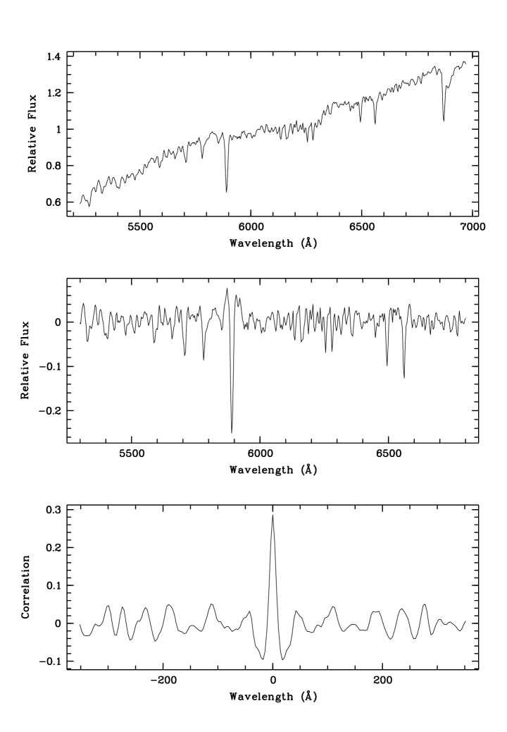
Figure 3: Top: Normalized spectrum of the star to be used as the cross-correlation template. Middle: The result of subtracting the continuum, applying a bandpass filter, and extracting the region of the spectrum that excludes atmospheric lines. Bottom: The cross-correlation function that results from correlating the template with itself. The shift of the central peak is approximately zero as expected.

A MIDAS script was written to perform the cross-correlation and extract the radial velocity information. Prior to performing the correlation, it is important to appropriately prepare a spectrum to reduce noise in the cross-correlation function. The first step in this process is to normalize the spectrum. Next, an eighth-order polynomial is fitted to the continuum and the continuum is subtracted. A bandpass filter is applied to the spectrum which excises both high and low spatial frequency components. The final step is to extract a large segment of the spectrum which excludes atmospheric absorption lines. These steps are shown in Figure 3 in which the template spectrum is cross-correlated with itself.

After cross-correlating the stellar spectrum with the template spectrum, the wavelength shift was determined from the position of the peak of the cross-correlation function. As amply demonstrated by the recent extra-solar planet detections through radial velocity measurements (see, eg., Butler et al. (1996)), the uncertainty in the radial velocity measurements through a cross-correlation technique can be substantially smaller than the spectral resolution, if the S/N in the spectrum is large and the choice of the template spectrum is appropriate. The central position of the cross-correlation peak was determined by fitting a gaussian which has an associated error. In order to determine the error in the cross-correlation process, it was necessary to take a cross-correlation for which the result was known and then add noise to one of the spectra. To do this, a program was written which takes a spectrum of reasonable S/N and cross-correlates the spectrum with itself several hundred times. With each iteration, various wavelength shifts and noise levels were simulated in the duplicate spectrum. The average difference between the calculated wavelength shift and the real wavelength shift was used to estimate the error in the cross-correlation process for different values of S/N. The results showed that the error in the cross-correlation is around 5 km/s and only becomes significant for very low S/N. Hence the cross-correlation algorithm is fairly robust, mostly due to the number of lines used. This error was combined with the error in the gaussian fit to estimate the total error in the radial velocity. The MIDAS cross-correlation script was also successfully tested by simulating line shifts in various spectra and by performing correlations on restricted wavelength ranges within a spectrum.

The template spectrum of the bright star was cross-correlated with the spectra of the lensed and the unlensed sources in each image, and their radial velocities were determined as outlined above.

4 RESULTS AND DISCUSSION

For each source an estimate of the spectral type, extinction, and relative radial velocity is made as discussed above. It is important to remember that the measurements of the microlensed sources apply only to the source and not the lens itself. The contribution of the lens is assumed to be small because the stellar mass function is biased towards lower masses and hence the lens is likely to be less massive and considerably fainter than the source (Mao et al., 1998). Low luminosity stars do not contribute significantly as sources since these would not normally be detected by the magnitude limited microlensing surveys.

Figure 4: Spectra (solid line) and fitted models (dashed line) for MACHO 95-BLG-17 and five non-microlensed stars in the field.

Table 3 gives the details of the observations, such as the grisms used, the date of observations, and the exposure times for all the observations. Table 5 shows the results of the analysis for all the observed microlensed sources. For the purpose of this table, the names of the events have been abbreviated, the first letter indicating the name of the collaboration and the following two numbers indicating the identity of the event. The results include the estimated spectral class, the color excess, and radial velocity, along with the uncertainties for each source.

For illustration, more details of the analysis procedure are presented for MACHO 95-BLG-17 which was observed with B150 and O150 grisms. For this event, the observed spectra of the microlensed source and five other stars in the field, along with their associated model spectra are shown in Figure 4. The results from fitting models to the spectra are given in Table 6. Shown in Figure 5 is the cross-correlation function for the spectrum when cross-correlated with the chosen radial velocity standard.

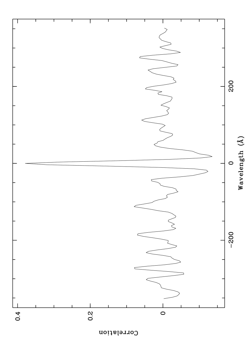
Figure 5: Cross-correlation function for the spectrum of MACHO 95-BLG-17.

The spectra of the remainder of the microlensed sources are shown in Figures 6–9. Note that most stars were fitted better by the lower metallicity models. This is an expected result since the Galactic bulge tends to be dominated by population II stars (Seeds, 1999).

Figure 6: Spectra of the microlensed sources DUO 95-BLG-2, MACHO 95-BLG-2, MACHO 95-BLG-3, and MACHO 95-BLG-4.

Figure 7: Spectra of the microlensed sources MACHO 95-BLG-8, MACHO 95-BLG-9, MACHO 95-BLG-10, and MACHO 95-BLG-12.

Figure 8: Spectra of the microlensed sources MACHO 95-BLG-13, MACHO 95-BLG-14, MACHO 95-BLG-18, and MACHO 95-BLG-19.

Figure 9: Spectra of the microlensed sources MACHO 95-BLG-30, OGLE 95-BLG-3, OGLE 95-BLG-7, and OGLE 95-BLG-16.

Unfortunately, our wavelength coverage is 3500-7000 Å, which is different from that of the MACHO collaboration. Furthermore, the spectrum by the MACHO group was obtained when the source was amplified. So the blending fraction (i.e., fraction of light from a possible blended object) may be different at the two epochs which may affect the result. And, as explained earlier, the limitations in the theoretical models make our spectral classifications uncertain if the spectral type is about M2 or later.

It would be interesting to compare our spectral classification with other such estimates available in the literature. There is one such source, MACHO 95-BLG-30, which has been studied in detail by the MACHO collaboration (Alcock et al., 1997) who obtained spectra with a wavelength coverage of 6230–9340 Å. From this they estimated a spectral type of M4III, which is close to and within uncertainties of our determination of M2III.

As explained earlier, our velocity determinations are relative and the absolute velocity can have large uncertainties because of the uncertainty in the absolute velocity of the template star. However, we are interested only on relative velocities in this study, which are more accurate as explained before.

4.1 Color-Magnitude Diagram Analysis

In carrying out a comparative study of the properties of the microlensed and non-microlensed sources, it is important to check the distributions of both samples of the sources in the color-magnitude diagram (CMD) since they can provide some insight into the sample being analyzed.

There have been several studies performed on Galactic bulge CMDs, such as Terndrup (1988) who was the first to use a CCD in this analysis. The OGLE collaboration has since presented CMDs of 14 fields surveyed in the direction of the Galactic bulge (Udalski et al., 1993). Some of the features common to these CMDs have been further studied, such as the well-defined red clump branch (Stanek et al., 1994) and the distribution of the disk stars (Paczyński et al., 1994a).

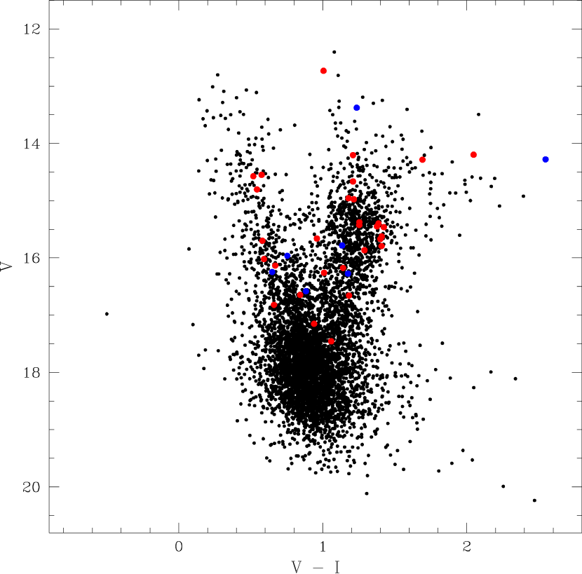
Figure 10: Combined color-magnitude diagram for the MACHO bulge fields 10, 12, 13, 17, 18, 19, and 30. The microlensed sources are shown in blue and the non-microlensed sources are shown in red.

During the 1995 observing season, photometric data from 7 of the 17 fields studied in this paper were obtained by the PLANET collaboration (Albrow et al., 1998). The CMDs for the individual fields have been combined into a single CMD, as shown in Figure 10. The combined CMD contains almost 22000 stars from the MACHO bulge fields 10, 12, 13, 17, 18, 19, and 30. Since the distribution of stars in the individual CMDs was almost identical, the colors and magnitudes were calibrated by adopting the position for the bulge red clump giants as estimated by Paczyński & Stanek (1998), who found an average $(V-I)$ for the red clump region of 1.22 and an average $I$ magnitude of 14.34. The microlensed sources are shown in blue in the CMD and the non-microlensed sources are shown in red.

The combined CMD is in good agreement with the CMDs published by OGLE. As expected, the CMD is dominated by bulge stars contained in a wide main sequence turnoff point and the red giant branch. Also visible in the diagram is a high concentration of stars in the blue part of the CMD, suggested to be dominated by disk stars (Paczyński et al., 1994a). The non-microlensed stars chosen for this study are of similar brightness to the microlensed sources. The combined CMD shows that these stars lie within the same sample as the microlensed sources and are generally located in the recognizable main sequence or red giant branch. Hence, the non-microlensed stars chosen for comparison in this study are fairly typical of the population towards the Galactic bulge and are suitable for use in this study.

It is of interest to compare the magnitudes and colors of the sources as derived from the CMD with the spectral classifications derived from the spectra. Shown in Table 7 are these results along with an estimate of the absolute magnitude $M_{V}$. The value of $M_{V}$ derived here assumes that the peak of the red clump is at $m_{I}=14.34$ and $(V-I)=1.22$, as found by Paczyński & Stanek (1998). This is equivalent to assuming that the star is approximately in the middle of the bulge corresponding to a distance modulus of 14.62. The error in $M_{V}$ is dominated by the intrinsic dispersion of the bulge stars, which is $\sigma_{V}\sim 1.5$ magnitudes. These results show that the luminosities measured from the CMD are roughly consistent with the classifications derived from the spectra and that giant stars have been preferentially selected since they are most likely to be in the Galactic bulge. Note that the magnitudes and colors shown in Table 7 are not the calibrated values but they are the expected dereddened magnitudes and colors if the sources were at the middle of the Galactic bulge. This also shows that the non-microlensed stars chosen here are also within the bulge and hence they form a good sample for our comparative study.

4.2 Extinctions of Microlensed vs. Non-microlensed Sources

Although the internal extinction within Baade’s window is thought to be small, there are large uncertainties. As discussed earlier, the microlensed sources will show an extinction offset relative to the unlensed stars if the extinction within the bulge is non-negligible. We note that almost all the sources (the microlensed as well as the comparison stars) are expected to be within the bulge, and that the sources lie within a fairly restricted region of the bulge ($0.55\arcdeg<l<3.98\arcdeg$ and $-4.92\arcdeg<b<-2.68\arcdeg$). Hence the foreground extinction caused by the Galactic disk (i.e., excluding the extinction within the bulge) is expected to be the same for all the sources. Thus, any extinction offset between the non-microlensed and microlensed samples would indicate that extinction within the bulge is non-negligible. As explained in paper I, this extinction offset can be used to estimate the fraction of bulge-bulge lensing.

Figure 11: Histogram of extinction values for microlensed and non-microlensed stars.

Shown in Figure 11 is a histogram of the extinction for microlensed and non-microlensed stars. There is a surprisingly large number of stars with little or no extinction amongst the non-microlensed stars which is most likely due to disk stars of low mass. This could be explained in part by the findings of Paczyński et al. (1994a) that indicate that there is an excess of disk stars by a factor of $\sim 2$ between us and a distance of 2.5 kpc towards the Galactic bulge, and a rapid drop by a factor of $\sim 10$ beyond that distance. The average extinction for the microlensed sources is $E_{B-V}=0.68$ and is $E_{B-V}=0.43$ for the non-microlensed stars. As expected, the distributions peak at these average values. The offset between the two mean values of $\Delta E_{B-V}=0.25$ is equivalent to a magnitude offset of $\approx 0.80$ in $V$.

To investigate the significance of the offset between the two mean values, a t-test was performed on the histogram data. A value of $t=3.07$ was obtained for 93 degrees of freedom which results in a probability of $p=0.01$. In other words, the difference in the mean values of the two distributions is significant at the 99% confidence level. To test how much weight is held by the unlensed stars with zero extinction, the t-test was performed again after removing these stars from the sample. This reduced the values to $t=2.42$ for 81 degrees of freedom which results in a probability of $\approx 0.02$, or significance at the 98% confidence level.

This test assumes a normal distribution for the data sets which is difficult to determine given the relatively small number of microlensed sources included in this sample. These results appear to agree with the previous discussions regarding the extinction bias of microlensed sources and a clear trend is seen in the presented histogram.

As explained in paper I, from the extinction distribution for microlensed sources it is possible to make an estimate of the fraction of bulge-bulge lensing. Using the formalism of paper I, a simple estimate of the fraction of bulge-bulge lensing is found to be $\sim 65\%$. This is consistent with earlier predictions based on the presence of the bar (Paczyński et al., 1994b; Zhao et al., 1995).

We now turn to another possible effect: the time scales of the microlensing events versus the extinction. For self-lensing within the bulge, the Einstein ring size increases if the distance between the lens and the source is larger. Since the microlensed sources are preferentially located at the far side of the bulge, the characteristic time scale should be longer for events exhibiting larger extinction if the internal extinction is important. However, the time scale of an event is also a function of the velocities of the lens and the source and so the time scale may depend upon the Galactic kinematics. If the velocity dispersion is the dominant component and is similar in different regions of the bulge then the time scale should be larger for a higher value of extinction. On the other hand, if rotation is the dominant component then the time scale may show a behavior which is only a small function of the extinction value.

Figure 12: Plot of the extinction of microlensed sources as a function of their characteristic time scales. Events exhibiting binary behavior are not included in this plot. Top: An abbreviated version of the event names is used to indicate the source positions. Bottom: A line of best fit to the points excluding events MACHO 95-BLG-3 and MACHO 95-BLG-13.

Shown in Figure 12 is a plot of the extinction of the microlensed sources as a function of their characteristic time scales. The top frame uses the abbreviated names of the events to show their positions on the plot and the bottom frame shows the corresponding data points with error bars. We should note that MACHO 95-BLG-13 is a very bright source and it has relatively low extinction. Therefore, it is almost certainly a disk star and hence should not be included in this analysis. MACHO 95-BLG-3 has an extremely short time scale which could mean that the source and the lens are very close to each other (both at the far side of the bulge), rather than a very small mass of the lens or a very high relative velocity. As indicated in paper I, this would make the event quite unusual and not typical of Galactic microlensing.

Rejecting these two anomalous points for the reasons expressed above, a line was fitted to the data using linear regression. This fit is shown in the bottom panel of Figure 12. The trend in this data shows that the velocity dispersion component of the Galactic kinematics is strong enough such that there is a correlation between the extinction and the characteristic time scale of the event. Linear regression was used to obtain a linear fit which produces the following equation for this trend

$$E_{B-V}=0.018\,t_{E}+0.13$$ (1)

Of course, contamination due to disk lensing will cause greater scatter in this result. This clear trend seems to further confirm the earlier result that the microlensed sources suffer from larger extinction and that they are predominantly at the far side of the bulge. We emphasize however, that the uncertainty in individual extinction measurements can be large. Furthermore, although there seems to be a clear linear trend, the trend is dominated by just two points, namely MACHO 95-BLG-02 and MACHO 95-BLG-10. Further observations will help in confirming this result.

4.3 Kinematics of Microlensed Sources

The microlensed sources provide a unique opportunity to investigate the kinematic properties in this region. The kinematic properties of our Galaxy have been studied and used with microlensing to construct consistent models of the Galaxy (Méra et al., 1998). It was suggested by Walker (1997) that one could use the kinematic properties of microlensed sources to distinguish between a lens population in the disk and a lens population in the bulge. It was also found that the radial velocity distributions between the two populations should not be substantially different for an axisymmetric bulge model but may exhibit a relative shift if the bulge is non-axisymmetric (barred), depending upon the kinematics of the bar. As we found in the previous section, the distribution of transverse velocities of these two populations should be substantially different.

Figure 13: Histogram of relative radial velocities for microlensed and non-microlensed stars.

Shown in Figure 13 is a histogram of the relative radial velocities for microlensed and non-microlensed stars. The average relative radial velocity for the microlensed sources is $v_{r}=-81.2$ and is $v_{r}=-71.5$ for the non-microlensed stars. There appears to be a slight shift between the peak values of these two distributions but this is well within the velocity dispersions of the sources, and given the small number of samples and the low-resolution of the spectra, this is not statistically significant.

To investigate the significance between the two mean values, a t-test was performed on the histogram data. A value of $t=0.52$ was obtained for 92 degrees of freedom which results in a very high probability that the difference in the mean values of the two distributions is not statistically significant.

This lack of correlation could be due to either of the following: (i) there is no intrinsic correlation, or (ii) the uncertainties in the velocity measurements is larger than estimated here, or (iii) the resolution is insufficient to see any correlation. Clearly, more spectroscopic observations with better S/N at a higher resolution will help in finding the exact cause.

We note that there was a significant difference between the extinction distributions for the microlensed and non-microlensed stars. Since there is no such difference between the radial velocity distributions, it is not expected that there will be a correlation between the extinction and radial velocity of the observed sources.

Figure 14: Plot of the extinction of all observed sources as a function of their relative radial velocities. The microlensed sources are shown as open circles and the non-microlensed sources are shown as crosses.

Shown in Figure 14 is a plot of the extinction of the microlensed and non-microlensed stars as a function of their relative radial velocities. This figure excludes only one star, namely star 3 from the MACHO 95-BLG-30 field, for which there were not enough spectral lines in the star’s B150 spectrum for an accurate estimate of the radial velocity. (For this source, the routine produced a relative radial velocity measurement of $v_{r}=-399.8\pm 14.1$, but this may be because of a misidentification of some spectral lines).

The microlensed sources are shown as circles and the non-microlensed sources are shown as crosses. As expected, there is an extinction shift between the microlensed population and the non-microlensed population but there is no apparent correlation between the extinction and the radial velocity. These results appear to agree with the postulates made by Walker (1997). These results are also expected since the total extinction varies depending upon the line of sight.

5 CONCLUSIONS

We have presented spectra of 17 microlensed sources taken with the EFOSC at the ESO 3.6m telescope. These spectra were used to derive the spectral type, extinction, and the radial velocities of these stars. Spectra were also taken of many non-microlensed sources in the same fields. The same analysis was done for the non-microlensed sources, and their spectral types, extinctions, and radial velocities were determined. This was carried out by developing MIDAS scripts to provide estimates of the extinction, spectral type, and radial velocity for each individual spectrum. A large library of Kurucz model spectra was constructed to model the spectra, and the radial velocities were measured relative to a bright star using the cross-correlation technique. These results are used for a comparative study of the physical properties of the microlensed and non-microlensed stars.

A comparison of the extinction distributions for microlensed and non-microlensed stars have been carried out through a statistical analysis. The average extinction for the microlensed sources is $E_{B-V}=0.68$ and is $E_{B-V}=0.43$ for the non-microlensed stars. The offset between the two mean values of $\delta E_{B-V}=0.25$ corresponds to a magnitude offset of $\delta A_{v}\approx 0.80$. A t-test performed on these distributions showed that the difference in the mean values of the two distributions is significant at the 99% confidence level.

A plot of the extinction of the microlensed sources as a function of their characteristic time scales shows that the sources with larger extinction, in general, correspond to larger time scales. This is consistent with the expectation that the sources with larger extinction lie farther along the line of sight.

The histogram presenting the relative radial velocities for microlensed and non-microlensed stars shows that the difference between the two distributions is not statistically significant. The sample needs to be increased to about 100 sources to detect any possible offset. Thus, more spectra of microlensed sources will be very useful in modeling the kinematics of the Galactic bulge. It is expected, however, that the transverse velocities of these two populations would be different. Hence it would be of great interest to determine the transverse velocities of the microlensed sources as these would, when combined with the radial velocities, contribute significantly to the knowledge of the kinematics of the far side of the Galactic bulge. It should be possible to make such measurements with the Hubble Space Telescope or with future space telescopes, such as NGST.

An estimate of the fraction of bulge-bulge lensing was made from the extinction distribution for microlensed sources. This simple method provides a rough estimate of the fraction of bulge-bulge lensing and is found to be $\sim 65\%$. This value is similar to the results obtained by previous investigations (Paczyński et al., 1994b; Zhao et al., 1995; Kiraga & Paczyński, 1994).

Table 1: Grisms used, their characteristics, and the rms deviations from the dispersion relation.

Grism	Wavelength Range (Å)	Dispersion (Å/pixel)	rms (pixels)
B150	3780–5510	3.3	0.18
B300	3740–6950	6.3	0.31
O150	5220–6980	3.4	0.19
R300	5890–9920	7.9	0.20

Table 2: Microlensing event information provided by the MACHO alerts and the OGLE and DUO publications. Information includes the coordinates of the sources, the baseline $V$ and $R$ magnitudes, and the characteristic time scales of the events.

Event	R.A. (J2000)	DEC. (J2000)	V	R	$t_{E}$ (days)
DUO-1995-BLL-2	18:10:17.2	-27:28:49	-	18.6	binary
MACHO 95-BLG-2	18:08:25.2	-27:58:38	19.0	17.9	61.0
MACHO 95-BLG-3	18:02:37.5	-29:39:36	18.7	17.6	1.0
MACHO 95-BLG-4	18:00:03.4	-29:11:04	18.1	17.1	3.5
MACHO 95-BLG-8	18:16:46.0	-26:11:43	17.1	16.3	15.5
MACHO 95-BLG-9	18:06:32.3	-30:55:55	17.2	16.2	12.0
MACHO 95-BLG-10	17:58:16.0	-29:32:11	18.9	18.0	47.5
MACHO 95-BLG-12	18:06:04.8	-29:52:38	18.6	17.7	binary
MACHO 95-BLG-13	18:08:47.0	-27:40:47	16.6	15.6	73.5
MACHO 95-BLG-14	18:01:26.3	-28:31:14	17.4	16.5	9.0
MACHO 95-BLG-17	18:03:01.1	-28:21:09	18.8	18.0	18.5
MACHO 95-BLG-18	18:07:20.6	-28:36:51	18.7	17.8	39.5
MACHO 95-BLG-19	18:11:32.5	-27:45:27	18.6	17.9	31.5
MACHO 95-BLG-30	18:07:04.3	-27:22:06	16.1	14.7	33.5
OGLE 95-BLG-3	18:04:43.5	-30:14:11	17.7	-	11.5
OGLE 95-BLG-7	18:03:35.8	-29:47:06	19.3	-	binary
OGLE 95-BLG-16	18:02:07.6	-30:01:12	20.0	-	26.2

Table 3: Summary of microlensing events observed. Information includes the date of observation (HJD - 2449000), the grisms used, and the respective exposure times.

Event	Obs. Date	Grisms Used	Exposure (seconds)
DUO 95-BUL-2	899.64	B150,O150	1800,2220
MACHO 95-BLG-2	899.89	O150	2280
MACHO 95-BLG-3	899.86	O150	1200
MACHO 95-BLG-4	899.84	O150	1800
MACHO 95-BLG-8	899.71	O150	2700
MACHO 95-BLG-9	899.78	O150	1800
MACHO 95-BLG-10	897.79	B150,O150	1800,1800
MACHO 95-BLG-12	897.74	B150,O150	1500,1200
MACHO 95-BLG-13	897.70	B150,O150,R300	900,600,120
MACHO 95-BLG-14	899.81	O150	1800
MACHO 95-BLG-17	898.69	B150,O150	1200,1800
MACHO 95-BLG-18	898.73	B150,O150	1800,1800
MACHO 95-BLG-19	897.85	B150,O150	1800,1800
MACHO 95-BLG-30	1251.75	B150,B300	1200,900
OGLE 95-BLG-3	899.75	O150	1800
OGLE 95-BLG-7	898.84	O150	2700
OGLE 95-BLG-16	898.79	B150,O150	1800,1800

Table 4: Coefficients for polynomial fits to $\log g$ values.

Class	a	b	c	d	e
I	$1.71\times 10^{-3}$	-0.05	0.37	-1.50	4.05
III	$5.75\times 10^{-3}$	-0.06	0.04	0.44	2.91
V	$9.30\times 10^{-3}$	-0.13	0.56	-0.80	4.30

Table 5: Classification, extinction, and relative radial velocity results for each of the observed microlensed sources.

Spectrum	Class	$E_{B-V}$	$v_{r}\,\mathrm{(km\,s^{-1})}$
D02	K2III	$0.22\pm 0.09$	$-97.3\pm 16.6$
M02	G2III	$1.19\pm 0.01$	$-210.7\pm 11.2$
M03	G0III	$1.31\pm 0.01$	$-37.6\pm 19.0$
M04	K0III	$0.63\pm 0.03$	$-46.7\pm 10.0$
M08	G0III	$0.61\pm 0.03$	$-21.9\pm 11.2$
M09	K4III	$0.39\pm 0.21$	$-34.2\pm 7.8$
M10	G2III	$0.99\pm 0.01$	$-41.1\pm 7.9$
M12	K0III	$0.58\pm 0.16$	$9.5\pm 8.0$
M13	K1I	$0.48\pm 0.07$	$-65.9\pm 9.1$
M14	K4III	$0.32\pm 0.06$	$-181.0\pm 11.4$
M17	G5III	$0.55\pm 0.04$	$-21.3\pm 6.6$
M18	K0III	$0.66\pm 0.09$	$-102.6\pm 6.9$
M19	G2III	$0.47\pm 0.11$	$-62.3\pm 8.8$
M30	M2III	$0.56\pm 0.02$	$-162.0\pm 22.7$
O03	K2I	$0.08\pm 0.01$	$-63.1\pm 11.3$
O07	G0III	$0.79\pm 0.02$	$-137.9\pm 11.5$
O16	G5III	$0.60\pm 0.01$	$-102.9\pm 10.0$

Table 6: Classification, extinction, and relative radial velocity results for the MACHO-1995-BLG-17 field.

Spectrum	Class	$E_{B-V}$	$v_{r}\,\mathrm{(km\,s^{-1})}$
Source	G5III	$0.55\pm 0.04$	$-21.3\pm 6.6$
Star 1	K3III	$0.42\pm 0.13$	$-72.1\pm 10.4$
Star 2	K5III	$0.33\pm 0.03$	$-150.1\pm 10.3$
Star 3	K2III	$0.64\pm 0.09$	$-72.1\pm 9.4$
Star 4	G2III	$0.29\pm 0.03$	$-182.1\pm 17.4$
Star 5	K2III	$0.46\pm 0.07$	$-180.9\pm 12.5$

Table 7: Classifications derived from spectra, dereddened apparent magnitudes and colors, and an estimate of the absolute magnitude for each of the microlensed and non-microlensed sources of interest included in the CMD.

Star	Classification	$m_{V}$	$V-I$	$M_{V}$
MB95010	G2III	16.25	0.65	1.63
Star 1	G0III	16.13	0.67	1.51
Star 2	K5III	14.28	1.69	-0.34
Star 4	K5III	15.67	1.40	1.05
Star 5	K3III	15.63	1.41	1.01
MB95012	K0III	16.27	1.18	1.65
Star 1	G2III	17.15	0.94	2.52
Star 2	K2III	15.86	1.29	1.24
Star 3	K3III	15.45	1.38	0.83
Star 4	G5V	16.82	0.66	2.20
Star 5	G2III	16.02	0.59	1.40
MB95013	K1I	13.38	1.24	-1.24
Star 1	K5III	15.40	1.39	1.78
Star 2	G2III	14.96	1.18	0.34
Star 3	K5III	15.38	1.25	0.76
Star 4	K5III	15.46	1.42	0.84
Star 5	K3III	15.43	1.25	0.81
MB95017	G5III	16.58	0.88	1.94
Star 1	G5III	14.57	0.52	-0.05
Star 3	G5III	15.70	0.58	1.08
MB95018	K0III	15.78	1.13	1.16
Star 1	K4III	14.66	1.21	0.04
Star 2	K2III	14.98	1.22	0.36
Star 3	K4III	15.79	1.41	1.17
Star 4	G5III	16.64	0.84	2.02
Star 5	K5III	14.20	2.04	-0.42
MB95019	G2III	15.96	0.75	1.34
Star 1	G5III	15.66	0.96	1.04
Star 2	G5III	17.45	1.06	2.83
Star 3	G8III	16.17	1.14	1.55
Star 4	K3III	16.66	1.18	2.04
Star 5	G8III	16.26	1.01	1.64
MB95030	M2III	14.28	2.55	-0.34
Star 1	G8III	14.80	0.54	0.28
Star 2	K3I	12.73	1.00	-1.89
Star 3	K1I	14.20	1.21	-0.42
Star 4	G5III	14.55	0.57	-0.07

References

- Alard et al. (1995) Alard, C., Mao, S., Guibert, J. 1995, A&A, 300, L17
- Albrow et al. (1998) Albrow, M., et al. 1998, ApJ, 509, 687
- Alcock et al. (1997) Alcock, C., et al. 1997, ApJ, 491, 436
- Bertelli et al. (1994) Bertelli, G., et al. 1994, A&AS, 106, 275
- Butler et al. (1996) Butler, R.P., et al. 1996, PASP, 108, 500
- Danks & Dennefeld (1994) Danks, A.C & Dennefeld, M. 1994, PASP, 106, 382
- Dravins (1999) Dravins, D. 1999, in Proc. IAU Symp. 170, “Precise Stellar Radial Velocities”, ed. J.B. Hearnshaw & C.D. Scarfe, p.268
- Feltzing & Gilmore (2000) Feltzing, S. & Gilmore, G. 2000, A&A, 355, 949
- Jacoby et al. (1984) Jacoby, G.H., Hunter, D.A., Christian, C.A. 1984, ApJS, 56, 257
- Kane, (2000) Kane, S.R. 2000, Ph.D. Dissertation, University of Tasmania, Hobart, Australia
- Kane & Sahu (2000) Kane, S.R. & Sahu, K.C. 2000, ApJ, submitted (astro-ph/0011383)
- Kiraga & Paczyński (1994) Kiraga, M. & Paczyński, B. 1994, ApJ, 430, L101
- Kurucz (1970) Kurucz, R. 1970, “Atlas: A computer program for calculating model stellar atmospheres”, SAO Special Report, Cambridge: Smithsonian Astrophysical Observatory
- Kurucz (1993) Kurucz, R. 1993, ATLAS9 Stellar Atmosphere Programs and 2 km/s grid. Kurucz CD-ROM No. 13. Cambridge, MA: Smithsonian Astrophysical Observatory
- Mao et al. (1998) Mao, S., Reetz, J., Lennon, D.J. 1998, A&A, 338, 56
- Méra et al. (1998) Méra, D., Chabrier, G., Schaeffer, R. 1998, A&A, 330, 937
- Mollerach & Roulet (1996) Mollerach, S. & Roulet, E. 1996, ApJ, 458, L9
- Morgan et al. (1943) Morgan, W.W., Keenan, P.C., Kellman, E. 1943, “An Atlas of Stellar Spectra with an Outline of Spectral Classification” (University of Chicago Press)
- Morse et al. (1991) Morse, J.A., Mathieu, R.D., Levine, S.E. 1991, AJ, 101, 1495
- Paczyński et al. (1994a) Paczyński, B., et al. 1994a, AJ, 107, 2060
- Paczyński et al. (1994b) Paczyński, B., et al. 1994b, ApJ, 435, L113
- Paczyński & Stanek (1998) Paczyński, B. & Stanek, K.Z. 1998, ApJ, 494, L219
- Schmidt-Kaler (1982) Schmidt-Kaler, T. 1982, BICDS, 23, 2
- Seaton (1979) Seaton, M.J. 1979, MNRAS, 187, 73p
- Seeds (1999) Seeds, M.A. 1999, Foundations of Astronomy (1999 ed.; Belmont, CA: Wadsworth Pub. Co)
- Stanek et al. (1994) Stanek, K.Z., et al. 1994, ApJ, 429, L73
- Stanek (1995) Stanek, K.Z. 1995, ApJ, 441, L29
- Stanek et al. (2000) Stanek, K.Z., et al. 2000, Acta Astron., 50, 191
- Terndrup (1988) Terndrup, D.M. 1988, AJ, 96, 884
- Tonry & Davis (1979) Tonry, J., Davis, M. 1979, AJ, 84, 1511
- Torres-Dodgen & Weaver (1993) Torres-Dodgen, A.V. & Weaver, W.B. 1993, PASP, 105, 693
- Udalski et al. (1993) Udalski, A., et al. 1993, Acta Astron., 43, 69
- Udry et al. (1999) Udry, S., et al. 1999, in Proc. IAU Symp. 170, “Precise Stellar Radial Velocities”, ed. J.B. Hearnshaw & C.D. Scarfe, p.383
- Walker (1997) Walker, M.A. 1997, MNRAS, 287, 629
- Woźniak & Szymański (1998) Woźniak, P., Szymański, M. 1998, Acta Astron., 48, 269
- Zhao et al. (1995) Zhao, H., Spergel, D.N., Rich, R.M. 1995, ApJ, 440, L13