Stellar Collisions and Blue Straggler Formation
Abstract
We review recent 3D hydrodynamic calculations of stellar collisions using the Smoothed Particle Hydrodynamics (SPH) method, and we discuss the implications of the results for the formation and evolution of blue stragglers in globular clusters. We also discuss the construction of simple analytic models for merger remnants, approximating the mass loss, shock heating, mixing, and angular momentum transport during a collision with simple algorithms that can be calibrated using our 3D hydrodynamic results. The thermodynamic and chemical composition profiles predicted by these simple models are compared with those from our SPH simulations, demonstrating that our new models provide accurate representations of true collisional merger remnants.
Vassar College, 124 Raymond Ave., Poughkeepsie, NY 12604-0562
MIT 6-201, Cambridge, MA 02139
1. Introduction
1.1. Stellar Interactions in Globular Clusters
In the cores of dense globular clusters, the stellar collision time can become comparable to the cluster lifetime, implying that essentially all stars must be affected by collisions (Hills & Day 1976). Stellar collisions have important consequences for the overall dynamical evolution of dense star clusters. The dissipation of kinetic energy in collisions and tidal encounters and the formation of more massive objects through mergers tend to accelerate core collapse. On the other hand, mass loss from evolving collision products can provide indirect heating of the cluster core, thereby slowing down core collapse.
In addition, in globular clusters, stellar collisions are thought to produce a variety of interesting observable objects at rates far exceeding those in the rest of the Galaxy. Low-mass X-ray binaries and recycled pulsars are thought to be formed through close dynamical interactions involving main-sequence or red-giant stars and neutron stars (see, e.g., Davies et al. 1992; Di Stefano & Rappaport 1992; Rasio & Shapiro 1991; Rasio et al. 2000). Cataclysmic variables are also expected to be produced through interactions involving white dwarfs (e.g., Di Stefano & Rappaport 1994; Davies 1997). Both white dwarfs and cataclysmic variables have now been detected directly in many clusters (Bailyn et al. 1996; Cool et al. 1998; Cool, in this volume; Edmonds et al. 1999; Richer et al. 1997).
Interactions involving main-sequence (MS) stars are thought to be related to the blue straggler phenomenon. Blue stragglers are objects that appear as MS stars above the turnoff point in the color-magnitude diagram (CMD) of a star cluster. All observations suggest that they are indeed massive MS stars formed through the merger of two (or more) lower-mass stars. In particular, Saffer et al. (1997) and Sepinsky et al. (2000) have directly measured the masses of several blue stragglers in the cores of 47 Tuc and NGC 6397 and confirmed that they are well above the MS turnoff mass (see also the article by Saffer in this volume). Gilliland et al. (1998) have demonstrated that the masses estimated from the pulsation frequencies of four oscillating blue stragglers in 47 Tuc are consistent with their positions in the CMD.
Mergers of MS stars can occur in at least two different ways: following the physical collision of two single stars, or through the coalescence of the two components in a close binary system (Bailyn 1995; Leonard 1989; Livio 1993). Direct evidence for binary progenitors has been found in the form of contact (W UMa type) binaries among blue stragglers in low-density globular clusters such as NGC 5466 (Mateo et al. 1990) and M71 (Yan & Mateo 1994), as well as in many open clusters (see Ahumada & Lapasset 1995 for a recent survey). At the same time, strong indication for a collisional origin comes from detections by HST of large numbers of blue stragglers concentrated in the cores of some of the densest clusters, such as M15 (De Marchi & Paresce 1994; Guhathakurta et al. 1996), M30 (Yanny et al. 1994; Guhathakurta et al. 1998), NGC 6624 (Sosin & King 1995), and M80 (Ferraro et al. 1999).
Collisions can happen directly between two single stars only in the cores of the densest clusters, but, even in moderately dense clusters, they can also happen indirectly, during resonant interactions involving primordial binaries (Bacon et al. 1996; Cheung et al. 2000; Davies & Benz 1995; Sigurdsson et al. 1994; Sigurdsson & Phinney 1995). Observational evidence for the existence of dynamically significant numbers of primordial binaries in globular clusters is well established (Côté et al. 1994; Hut et al. 1992; Rubenstein & Bailyn 1997). Dynamical interactions between hard primordial binaries and other single stars or binaries are thought to be the primary mechanism for supporting a globular cluster against core collapse (Gao et al. 1991; Goodman & Hut 1989; Rasio 2000). In addition, exchange interactions between primordial binaries and compact objects can explain very naturally the formation in globular cluster cores of large numbers of X-ray binaries and recycled pulsars (see, e.g., Rasio, Pfahl, & Rappaport 2000 and references therein).
In all clusters, dynamical interactions between primordial binaries can result in dramatically increased collision rates. This is because the interactions are often resonant, with all four stars involved remaining together in a small volume for a long time ( orbital times). For example, in the case of an interaction between two typical hard binaries with semi-major axes AU containing MS stars, the effective cross section for collision between any two of the four stars involved is essentially equal to the entire geometric cross section of the binaries (Bacon et al. 1996; Cheung et al. 2000). This implies a collision rate times larger than what would be predicted for single stars. Collisions involving more than two stars can be quite common during binary–binary interactions, since the product of a first collision between two stars expands adiabatically following shock heating, and therefore has a larger cross section for subsequent collisions with one of the other two stars (Cheung et al. 2000). These multiple collisions provide a natural explanation for the existence of blue stragglers that may have masses above twice the turnoff mass (Saffer, in this volume; Sepinsky et al. 2000).
1.2. Hydrodynamic Calculations of Stellar Mergers
Benz & Hills (1987; 1992) performed the first 3D calculations of direct collisions between two MS stars, using the Smoothed Particle Hydrodynamics (SPH) method. An important conclusion of their pioneering study was that stellar collisions could lead to thorough mixing of the fluid. In particular, they pointed out that the mixing of fresh hydrogen fuel into the core of the merger remnant could reset the nuclear clock of a blue straggler, allowing it to remain visible for a full MS lifetime yr after its formation. In subsequent work it was generally assumed that the merger remnants resulting from stellar collisions were nearly homogeneous. Blue stragglers would then start their life close to the zero-age MS, although with an anomalously high helium abundance coming from the hydrogen burning in the parent stars. In contrast, little hydrodynamic mixing was expected to occur during the much gentler process of binary coalescence, which could take place on a stellar evolution timescale rather than on a dynamical timescale (Bailyn 1992; Mateo et al. 1990).
On the basis of these ideas, Bailyn (1992) suggested a way of distinguishing observationally between the two possible formation processes. Blue stragglers made from collisions would have a higher helium abundance in their outer layers than those made from binary mergers, and this would generally make them appear somewhat brighter and bluer. A detailed analysis was carried out by Bailyn & Pinsonneault (1995), who performed the first stellar evolution calculations for blue stragglers assuming various initial chemical composition profiles. To represent the collisional case, chemically homogeneous initial profiles with enhanced helium abundances were assumed. For the dense cluster 47 Tuc, the observed luminosity function and numbers of blue stragglers appeared to be consistent with a collisional origin.
Lombardi, Rasio, & Shapiro (1995, 1996) later re-examined the question of hydrodynamic mixing during stellar collisions, using higher-resolution SPH calculations. They found that, in contrast to previous results, hydrodynamic mixing during collisions may be very inefficient, and typical merger remnants produced by collisions could be far from chemically homogeneous. In the case of collisions between two nearly identical stars, the final chemical composition profile is in fact very close to the initial profile of the parent stars (Lombardi, Rasio, & Shapiro 1995; Rasio 1996a). For two turnoff stars, this means that the core of the merger remnant is mostly helium. Prompted by these results, Sills, Bailyn & Demarque (1995) started investigating the possible consequences of blue stragglers being born unmixed. Using stellar structure calculations, they compared the predicted colors and luminosities of initially unmixed models with observations of the six very bright blue stragglers in the core of NGC 6397. They concluded that some of these blue stragglers have observed colors that cannot be explained using unmixed initial models (cf. Ouellette & Pritchet 1998). Initially homogeneous models, however, could reproduce all the observations. In addition, unmixed models have very short MS lifetimes and may be generally incompatible with the observed numbers of blue stragglers in dense cluster cores. The key to resolving this apparent inconsistency may be stellar rotation, which can both provide more mixing and increase the stellar evolution lifetime of collision products (Sills et al. 2000; Sills, in this volume).
Our most recent hydrodynamic calculations (Sills & Lombardi 1997; Sills et al. 2000) improve on previous studies (Benz & Hills 1987, 1992; Lombardi et al. 1995, 1996; Sandquist et al. 1997) by adopting more realistic initial stellar models and by performing numerical calculations with increased spatial resolution. The latest version of our SPH code has been fully parallelized and allows calculations to be performed with SPH particles, compared to the used in previous studies. All spurious transport processes affecting SPH calculations can be reduced significantly by increasing the number of SPH particles (Lombardi et al. 1999). For the first time in a study of stellar collisions, accurate initial stellar models have been calculated using a state-of-the-art stellar evolution code (the YREC code developed at Yale by Demarque and collaborators; see Guenther et al. 1992 and Sills et al. 2000). This allows us, in particular, to study chemical mixing and stellar evolution of collision products in a completely self-consistent way. The importance of using realistic initial models (rather than simple polytropes, which were used in all previous studies) in stellar collision calculations was demonstrated by Sills & Lombardi (1997). In some cases, results based on calculations for polytropes can actually lead to qualitatively incorrect conclusions about the structure of the merger remnant.
The vast majority of 3D numerical studies of stellar collisions have used the SPH method (see, e.g., Monaghan 1992 and Rasio & Lombardi 1999 for recent reviews). Indeed, because of its Lagrangian nature, SPH presents some clear advantages over more traditional grid-based methods for calculations of stellar interactions. Most importantly, fluid advection, even for stars with a sharply defined surface, is accomplished without difficulty in SPH, since the particles simply follow their trajectories in the flow. In contrast, to track accurately the orbital motion of two stars across a large 3D grid can be quite tricky, and the stellar surfaces then require a special treatment (to avoid “bleeding”). A Lagrangian scheme is also ideal for following hydrodynamic mixing, since the chemical composition attached to each particle is simply advected with that particle. This is a key advantage for the problems discussed here, where the chemical composition profiles of merger remnants must be determined accurately. SPH is also very computationally efficient, since it concentrates the numerical elements (particles) where the fluid is at all times, not wasting any resources on emty regions of space. For this reason, with given computational resources, SPH can provide higher averaged spatial resolution than grid-based calculations, although Godunov-type schemes such as PPM typically provide better resolution of shock fronts. SPH also makes it easy to track the hydrodynamic ejection of matter to large distances from the central dense regions. This is a key advantage for calculating processes such as collisions, where ejection of significant amounts of matter through rotational instabilities or gas shocking plays an important role. Sophisticated nested-grid algorithms and more expensive calculations are necessary to accomplish the same with grid-based methods.
Spurious transport by SPH particles can render completely unphysical the results of low-resolution hydrodynamics calculations. For example, particle shear viscosity can lead to the artificial generation of vorticity. The strong differential rotation observed in collision products could also be damped rapidly, leading to spurious transport of angular momentum away from the central region. In addition, numerical viscosity can also lead to spurious entropy production and this contributes systematic errors in all thermodynamic properties of the fluid. When studying chemical mixing during mergers, it is particularly important to calibrate how much of the observed mixing is real, and how much results from spurious diffusion of SPH particles. Based on a very extensive study with test calculations (Lombardi et al. 1999), we are confident that, with SPH particles, and with the latest improvements to our code (see Lombardi et al. 1999 for details), spurious transport processes can be brought down to an acceptable level.
1.3. Thermal Relaxation and Stellar Evolution of Merger Remnants
Hydrodynamic calculations are of course limited to following the evolution of mergers on a dynamical timescale (hours for MS stars) but are not capable of following processes taking place on a thermal timescale (yr for MS stars). The final configurations obtained at the end of hydrodynamic calculations are very close to hydrostatic equilibrium, but are generally far from thermal equilibrium. Therefore, the merger remnant will need to contract (on its Kelvin time ) before it can be treated as a star again. This thermal relaxation of an object initially far from equilibrium cannot be calculated with most standard stellar evolution codes, which assume small departures from thermal equilibrium. However, to compute theoretically the subsequent stellar evolution of the object, and to make comparisons with observations, it is necessary to perform detailed calculations of this thermal relaxation phase, taking into account processes that are not always incorporated into existing stellar evolution codes. As the object evolves towards thermal equilibrium, many processes can lead to additional mixing of the fluid. In particular, thermal convection, which is well known to occur during the evolution of ordinary pre-MS stars, could produce significant mixing in blue stragglers (see Leonard & Livio 1995). Even if ordinary convection does not occur, local thermal instabilities such as semi-convection and thermohaline-type instabilities (Spruit 1992) can develop, leading to mixing on the local radiative damping timescale. Indeed, some of our previous hydrodynamic calculations (Lombardi et al. 1996) suggest that many merger remnants, although convectively stable, have temperature and chemical composition profiles with large thermally unstable regions. For the rapidly (and differentially) rotating products of grazing collisions, meridional circulation, as well as various rotationally-induced instabilities (see, e.g., Tassoul 1978), can lead not only to mixing, but also to angular momentum transport and mass loss. Loss of angular momentum through magnetic braking or coupling of the star to an outer disk of ejected material could also play an important role in spinning down the merger remnant.
For each final configuration obtained with our SPH code, we calculate the thermal relaxation of the remnant using a modified version of the Yale stellar evolution code (YREC, see Sills at al. 2000 and Sills, in this volume), which follows the evolution of a rotating star both on a thermal timescale and on a nuclear timescale (Sills 1998). YREC evolves a star through a sequence of models of increasing age, solving the linearized stellar evolution equations for interior profiles such as chemical composition, pressure, temperature, density and luminosity. All relevant nuclear reactions (including pp-chains, the CNO cycle, triple- reactions and light element reactions) are treated. Recent opacity tables are used (ensuring that the remnant’s position in a CMD can be accurately determined). YREC incorporates standard treatments of convection, semi-convection and rotationally-induced mixing and angular momentum transport through processes such as dynamical and secular shear instabilities, meridional circulation, and the Goldreich-Schubert-Fricke instability (see Guenther et al. 1992 for details). The free parameters in the code (the mixing length and parameters that set the efficiency of angular momentum transport and rotational chemical mixing) are set by calibrating a solar mass and solar metallicity model to the Sun. For blue stragglers, the various transport processes can potentially carry fresh hydrogen fuel into the stellar core and thereby extend the MS lifetime of the remnant. Furthermore, any helium mixed into the outer layers affect the opacity and hence the remnant’s position in a CMD.
This treatment, combining hydrodynamics and stellar evolution, attempts to provide a complete, self-consistent description of blue straggler formation and evolution, assuming a collisional origin. Our first results demonstrating the feasibility of this basic approach have been presented in Sills et al. (2000; see also Sills, in this volume). These results, although encouraging, have revealed a number of important theoretical problems that will have to be addressed carefully in future work. Most importantly, we find that even slightly off-axis collisions produce merger remnants that can be rotating near break-up. As they contract to the MS, these objects must lose some mass and a large amount of angular momentum. The most likely angular momentum loss mechanism, which we plan to study in detail, is magnetic coupling to an outer disk (containing the material ejected during the initial collision). Ordinary magnetic braking (as in pre-MS stars) is not likely to be important since, at least based on the calculations we performed so far, typical merger remnants never develop outer convective envelopes.
2. SPH Calculations of Stellar Collisions
2.1. Implementation of the SPH Code
Our most recent hydrodynamic calculations have been done using a new, parallel version of the SPH code developed originally by Rasio (1991) specifically for the study of hydrodynamic stellar interactions (see, e.g., Faber & Rasio 2000; Lai et al. 1993; Lombardi et al. 1995, 1996; Rasio & Livio 1996; Rasio & Lombardi 1999; Rasio & Shapiro 1991, 1992, 1995).
The gravitational field in our code is calculated on a 3D grid using an FFT-based convolution algorithm. The density field is placed on a 3D grid by a cloud-in-cell method, and convolved with a kernel function calculated once during the initialization of the simulation. We use zero-padding of our grids to obtain correct boundary conditions for an isolated system, at the expense of memory storage. Gravitational forces are calculated from the gravitational potential by finite differencing on the grid, and then interpolated for each particle using the same cloud-in-cell assignment. For most problems, the CPU time is dominated by the calculation of the gravitational field. The current implementation is based on the high-performance FFTW parallel routines (Frigo & Johnson 1997). Our SPH code was parallelized using MPI (the message passing interface), to run efficiently on multiple processors. In benchmarking tests, we have found that our parallel code scales very well when using up to processors on a distributed shared-memory supercomputer. Our parallel code now allows us to perform SPH calculations using up to particles, which provides a spatial resolution for colliding stars of radius . For more details on the current implementation of our parallel code, see Faber & Rasio (2000).
Local densities and hydrodynamic forces at each particle position are calculated by smoothing over nearest neighbors. The size of each particle’s smoothing kernel is evolved in time to keep close to a predetermined optimal value. For the high-resolution calculations in this paper the optimal number of neighbors was set at . Neighbor lists for each particle are recomputed at every iteration using a linked-list, grid-based parallel algorithm. Note that neighborhood is not a symmetric property, as one particle can be included in another’s neighbor list but not vice versa. Pressure and artificial viscosity forces are calculated by a “gather-scatter” method, looping over all particles in turn, gathering the force contribution on each particle from its neighbors, and scattering out the equal and opposite force contribution on the neighbors from each particle.
A number of variables are associated with each particle , including its mass , position , velocity , entropic variable and numerical smoothing length . The entropic variable is a measure of the fluid’s compressibility and is closely related (but not equal) to specific entropy: for example, both and specific entropy are conserved in the absence of shocks. For convenience, we refer to simply as “entropy.” In this paper we adopt an equation of state appropriate for a monatomic ideal gas: the adiabatic index and , where and are the density and pressure of particle .
The equation of motion for the SPH particles can be written as
| (1) |
where is the gravitational acceleration and
| (2) |
The summation in equation (2) is over neighbors and is a symmetrized smoothing kernel (see Rasio & Lombardi 1999 for details). The artificial viscosity (AV) term ensures that correct jump conditions are satisfied across (smoothed) shock fronts, while the rest of equation (2) represents one of many possible SPH-estimators for the acceleration due to the local pressure gradient (see, e.g., Monaghan 1985).
The rate of increase, due to shocks, for the entropy of particle is given by
| (3) |
We adopt the form of AV proposed by Balsara (1995):
| (4) |
where
| (5) |
The terms and are, respectively, the average smoothing length and sound speed associated with particles and . Here is the so-called form function for particle , defined by
| (6) |
where
| (7) |
and
| (8) |
The function acts as a switch, approaching unity in regions of strong compression () and vanishing in regions of large vorticity (). Consequently, this AV has the advantage that it is suppressed in shear layers. In this paper we use , and . This choice of AV treats shocks well, while introducing only relatively small amounts of numerical viscosity (Lombardi et al. 1999).
For stability, the timestep must satisfy a modified Courant condition, with replacing the usual grid separation. For accuracy, the timestep must be a small enough fraction of the dynamical time. To determine the timestep, we follow the prescription proposed by Monaghan (1989), which allows for an efficient use of computational resources. This method sets
| (9) |
where the constant dimensionless Courant number typically satisfies , and where
| (10) | |||||
| (11) |
with being a constant of order unity.
Our simulations employ equal-mass SPH particles, both to keep the resolution high in the stellar cores and to minimize spurious mixing during the simulation (see Lombardi et al. 1999 for a discussion of spurious transport induced by unequal mass particles). Due to extreme central densities in the parent stars (especially turnoff stars), the Courant stability condition requires exceedingly small timesteps. Consequently, an elapsed physical time of one hour in our high-resolution calculations can require roughly 1000 iterations and 100 CPU hours on an SGI/Cray Origin2000 supercomputer.
2.2. Initial Conditions
All our recent simulations use parent star models calculated with YREC, as discussed in Sills & Lombardi (1997) and Sills et al. (2000). In particular, we have evolved (non-rotating) MS stars of total mass and with a primordial helium abundance and metallicity for 15 Gyr, the amount of time needed to exhaust the hydrogen at the center of the star (a typical globular cluster turnoff mass). The total helium mass fractions for the and parent stars are 0.286 and 0.395, and their radii are and , respectively. From the pressure and density profiles of these models, we compute the entropy profile and assign values of to SPH particles accordingly. In addition, the chemical abundance profiles of 15 different elements are used to set the composition of the SPH particles. To minimize numerical noise, each parent star’s SPH model is relaxed to equilibrium using an artificial drag force on the particles, and then these relaxed models are used to initiate the collision calculations.
The stars are initially non-rotating and separated by , where is the radius of the turnoff () star. The initial velocities are calculated by approximating the stars as point masses on an orbit with zero orbital energy and a pericenter separation . A Cartesian coordinate system is chosen such that these hypothetical point masses of mass and would reach pericenter at positions , , where and refers to the more massive star. The orbital plane is chosen to be . With these choices, the center of mass resides at the the origin.
2.3. Sample of Numerical Results
Table 1 summarizes the parameters and results of the simulations presented in this section. The first column gives the name by which the calculation is referred to in this paper; we use lower-case letters to distinguish the present calculations from the corresponding calculations involving polytropic parent stars presented in Lombardi et al. (1996). The second and third columns give the masses and of the parent stars. Column (4) gives the ratio , where is the pericenter separation for the initial orbit and is the sum of the two (unperturbed) stellar radii. This ratio has the value for a head-on collision, and for a grazing encounter. Column (5) gives the number of SPH particles. Column (6) gives the final time at which the calculation was terminated. Column (7) gives the total angular momentum of the merger remnant. Column (8) gives the ratio of rotational kinetic energy to gravitational binding energy of the (bound) merger remnant in its center-of-mass frame at time . Since the amount of mass ejected during a parabolic collision is quite small, the merger remnant never acquires a large recoil velocity. The Case e, f and k simulations implemented neighbors per particle on average, while Case j′ implemented an average of 32 neighbors per particle. Case j′ is a low-resolution calculation of a nearly head-on collision used in Sills et al. (2000) to help demonstrate the applicability of our approach for converting the final SPH remnant model to a YREC starting model.
| Case | |||||||
|---|---|---|---|---|---|---|---|
| [hours] | [g cm2 s-1] | ||||||
| (1) | (2) | (3) | (4) | (5) | (6) | (7) | (8) |
| e | 0.8 | 0.6 | 0.25 | 11.10 | 0.101 | ||
| f | 0.8 | 0.6 | 0.50 | 24.64 | 0.119 | ||
| k | 0.6 | 0.6 | 0.25 | 11.10 | 0.085 | ||
| j′ | 0.6 | 0.6 | 0.01 | 9.25 | 0.005 |
Figure 1 illustrates the dynamical evolution of the entropy in the orbital plane for case e: a terminal age main-sequence star () collides with a slightly less massive star (). The parabolic trajectory has a pericenter separation . The first collision occurs hours after the initial configuration of the calculation. The impact disrupts the outer layers of the two parents, but leaves their inner cores essentially undisturbed. The two components withdraw to apocenter at hours, with a bridge of low entropy fluid from the smaller parent connecting the cores. As the cores fall back towards one another and merge, a complicated shock heating pattern ensues, with the strongest shocks occurring near the leading edge of the fluid from the smaller parent. The cores themselves are largely shielded from the shock heating, and the lowest entropy fluid settles down to the center as the remnant approaches dynamical equilibrium. The merger remnant is rapidly and differentially rotating, and shear makes the bound fluid quickly approach axisymmetry within a few dynamical timescales. Visualizations of our collision calculations can be found at http://research.amnh.org/summers/scviz/lombardi.html.
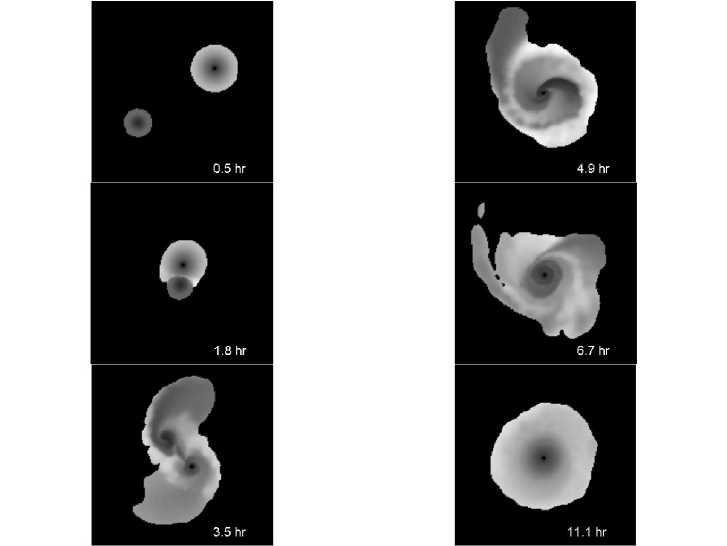
Figure 2 shows contours of density , entropy and component of the specific angular momentum for each collision remnant in a slice containing its rotation axis. The contours shown represent an average over the azimuthal angle, as the remnant approaches axisymmetry at the end of the simulation. The conditions for dynamical stability against axisymmetric perturbations are that (1) the entropy never decreases outward, and (2) on each constant surface, the specific angular momentum increases from the poles to the equator (the Hoiland criterion; see, e.g., Tassoul 1978, Chap. 7). Both of these conditions are met throughout the preponderance of mass in our remnant models.

Figure 2 also reveals that for our rapidly rotating remnants (cases e, f and k) the specific angular momentum (and hence the angular velocity , related by ) varies significantly on the cylindrical surfaces of constant . These rotating remnants are therefore not barotropes, by definition. For a rotating, chemically homogeneous star, stable thermal equilibrium requires , where is measured along the direction of the rotation axis (the Goldreich-Schubert criterion; see, e.g., Tassoul 1978, Chap. 7). In chemically inhomogeneous stars, regions with a sufficiently large and stabilizing composition gradient can in principle still be thermally stable even with . However, all of our remnants, rotating or not, are far from thermal equilibrium.
To convert our fully three-dimensional hydrodynamic results into the one-dimensional YREC format, we first average the entropy and specific angular momentum values in bins in enclosed mass fraction. With the and profiles given, the structure of the rotating remnant is uniquely determined in the formalism of Endal and Sofia (1976), by integrating the general form of the equation of hydrostatic equilibrium [see their eq. (9)]. To do so, we implement an iterative procedure in which initial guesses at the central pressure and angular velocity are refined until a self-consistent YREC model is converged upon. Although the pressure, density, and angular velocity profiles of the resulting YREC model cannot also be simultaneously constrained to equal the corresponding (averaged) SPH profiles, the differences are slight (see, for example, the profiles in Figure 3). Indeed, the subsequent evolutionary tracks are not significantly different for remnant models that use the form of the profile taken directly from SPH.

Examples of results from YREC integrations for collision products and predictions for the location of rotating blue stragglers in the CMD are presented in the article by Sills (in this volume).
3. Simple Models for Merger Remnants
The results of our hydrodynamic calculations can be used to construct a set of simple analytic fitting formulae that can be used in other studies to construct approximate models for stellar collision products, without resorting to full hydrodynamic calculations. In particular, these results can be used in studies of dense star cluster dynamics that take into account the important effects of stellar collisions on the overall dynamical evolution of the cluster, and in scattering experiments for binary–single and binary–binary interactions that take into account the (very frequent) stellar collisions occurring during resonant interactions (instead of the far more costly approach of running a low-resolution SPH simulation each time a collision takes place; cf. Davies et al. 1994).
We begin with two (non-rotating) parent star models, specifying initial profiles for the stellar density , pressure , and abundance of chemicals. The profile for the entropic variable can also be calculated easily and is of central importance. Fluid elements with low values of sink to the bottom of a gravitational potential well, and the profile of a star in stable dynamical equilibrium increases radially outwards. Indeed, it is easy to show that the condition is equivalent to the usual Ledoux criterion for convective stability of a nonrotating star (Lombardi et al. 1996). Since the quantity depends only on the chemical composition and the entropy, it remains constant in the absence of shocks. Our algorithms are based upon closely modeling the results of SPH calculations presented in Lombardi et al. (1996) (for collisions of polytropic stars) as well as in Sills & Lombardi (1997) and §2.3 of this paper (for collisions of more realistically modeled stars). We model mass loss, shock heating, fluid mixing, and the angular momentum distribution.
3.1. Mass Loss
The velocity dispersion of globular cluster stars is typically only km s-1, which is much smaller than the escape velocity from the surface of a MS star [for example, a star of mass and radius has an escape velocity km s-1]. For this reason, collisional trajectories are well approximated as parabolic, and the mergers are relatively gentle: the mass lost is never more than about 8% of the total mass in the system (mass loss with hyperbolic trajectories is treated by Lai, Rasio, & Shapiro 1994). Furthermore, most main sequence stars in globular clusters are not rapidly rotating, and it is a good approximation to treat the initial parent stars as non-rotating.
Given models for the parent stars (see Table 2), we first determine the mass lost during a collision. Inspection of hydrodynamic results for collisions between realistically modeled stars, as well as for collisions between polytropes, suggests that the fraction of mass ejected can be estimated approximately by
| (12) |
where and are dimensionless constants which we take to be 0.1 and 3, is the reduced mass of the parent stars, is the radius of parent star , is the radius of parent star at an enclosed mass fraction , and is the periastron separation for the initial parabolic orbit. While developing equation (12) we searched for a relation that accounted for the mass distribution (not just the total masses and radii) of the parent stars in some simple way. The more diffuse the outer layers of the parents, the longer the stellar cores are able to accelerate towards each other after the initial impact: the in the denominator of equation (12) accounts for this increased effective collision speed for parents whose mass distributions are centrally concentrated. The dependence on in equation (12) arises from the expectation that the mass loss will be roughly proportional to the kinetic energy at impact, and from the fact that a simple rescaling of the stellar masses () in a hydrodynamic simulation leaves unchanged. This method yields remnant masses which are seldom more than different than what is given by a hydrodynamic simulation (see the last two columns of Table 3); this is clearly a significant improvement over neglecting mass loss completely, which sometimes can overestimate the remnant mass by more than .
We distribute the mass loss between the two parent stars in such a way that the outermost fluid layers of each parent which are retained in the remnant have the same entropic variable .
| Structure type | |||
|---|---|---|---|
| Polytropic | 0.8 | 0.955 | 0.38 |
| Polytropic | 0.6 | 0.54 | 0.36 |
| Polytropic | 0.4 | 0.35 | 0.25 |
| Polytropic | 0.16 | 0.15 | 0.11 |
| Realistic | 0.8 | 0.955 | 0.284 |
| Realistic | 0.6 | 0.517 | 0.262 |
| Realistic | 0.4 | 0.357 | 0.227 |
| Casea | b | c | d | e | |||
|---|---|---|---|---|---|---|---|
| A | 0.8 | 0.8 | 0.00 | 0.064 | 0.063 | 1.50 | 1.50 |
| B | 0.8 | 0.8 | 0.25 | 0.023 | 0.022 | 1.56 | 1.57 |
| C | 0.8 | 0.8 | 0.50 | 0.012 | 0.013 | 1.58 | 1.58 |
| D | 0.8 | 0.6 | 0.00 | 0.057 | 0.050 | 1.32 | 1.33 |
| E | 0.8 | 0.6 | 0.25 | 0.024 | 0.020 | 1.37 | 1.37 |
| F | 0.8 | 0.6 | 0.50 | 0.008 | 0.012 | 1.39 | 1.38 |
| G | 0.8 | 0.4 | 0.00 | 0.056 | 0.046 | 1.13 | 1.14 |
| H | 0.8 | 0.4 | 0.25 | 0.028 | 0.018 | 1.17 | 1.18 |
| I | 0.8 | 0.4 | 0.50 | 0.008 | 0.011 | 1.19 | 1.19 |
| J | 0.6 | 0.6 | 0.00 | 0.049 | 0.038 | 1.14 | 1.16 |
| K | 0.6 | 0.6 | 0.25 | 0.028 | 0.018 | 1.17 | 1.18 |
| L | 0.6 | 0.6 | 0.50 | 0.022 | 0.012 | 1.17 | 1.19 |
| N | 0.6 | 0.4 | 0.25 | 0.029 | 0.017 | 0.97 | 0.98 |
| O | 0.6 | 0.4 | 0.50 | 0.010 | 0.011 | 0.99 | 0.99 |
| P | 0.4 | 0.4 | 0.00 | 0.037 | 0.035 | 0.77 | 0.77 |
| Q | 0.4 | 0.4 | 0.25 | 0.029 | 0.017 | 0.78 | 0.79 |
| R | 0.4 | 0.4 | 0.50 | 0.010 | 0.011 | 0.79 | 0.79 |
| S | 0.4 | 0.4 | 0.75 | 0.008 | 0.008 | 0.79 | 0.79 |
| T | 0.4 | 0.4 | 0.95 | 0.011 | 0.007 | 0.79 | 0.79 |
| U | 0.8 | 0.16 | 0.00 | 0.026 | 0.031 | 0.94 | 0.93 |
| V | 0.8 | 0.16 | 0.25 | 0.025 | 0.012 | 0.94 | 0.95 |
| W | 0.8 | 0.16 | 0.50 | 0.021 | 0.007 | 0.94 | 0.95 |
| a | 0.8 | 0.8 | 0.00 | 0.080 | 0.084 | 1.47 | 1.47 |
| e | 0.8 | 0.6 | 0.25 | 0.029 | 0.022 | 1.36 | 1.37 |
| f | 0.8 | 0.6 | 0.50 | 0.014 | 0.013 | 1.38 | 1.38 |
| g | 0.8 | 0.4 | 0.00 | 0.063 | 0.057 | 1.12 | 1.13 |
| k | 0.6 | 0.6 | 0.25 | 0.032 | 0.020 | 1.16 | 1.18 |
3.2. Shock Heating
Shocks increase the value of the fluid’s entropic variable (see eq. 3). The distribution and timing of shock heating during a collision involve numerous complicated processes (see Fig. 1): an initial shock front is generated at the interface between the stars during impact, the oscillating merger remnant sends out waves of shock rings, and finally the outer layers of the remnant are shocked as gravitationally bound ejecta fall back to the remnant surface. Our goal is not to derive approximations describing the shock heating during each of these stages, but rather empirically to determine physically reasonable relations which fit the available SPH data.
Let and be, respectively, the final and initial values of the entropic variable for some particular fluid element. We used the results of hydrodynamic calculations to examine how the change , as well as the ratio , depended on a variety of functions of (the initial pressure) and . Our search for a simple means of modeling this dependence was guided by a handful of features evident from hydrodynamic simulations: (1) fluid deep within the parents are shielded from the brunt of the shocks, (2) in head-on collisions, fluid from the less massive parent experiences less shock heating than fluid with the same initial pressure from the more massive parent, (3) in off-axis collisions with multiple periastron passages before merger, fluid from the less massive parent experiences more shock heating than fluid with the same initial pressure from the more massive parent, and (4) the amount of shock heating for each parent clearly must be the same if the two parent stars are identical.
We find that when is plotted versus , the resulting curve for each parent star was fairly linear (see Fig. 4) with a slope of approximately throughout most of the remnant in the simulations we examined:
| (13) |
Here the intercept is a function of the periastron separation for the initial parabolic trajectory as well as the masses and of the parent stars. Larger values of correspond to larger amounts of shock heating in star , where the index for the more massive parent and for the less massive parent (). For simplicity of notation, we have suppressed the index on the , and in equation (13).

The SPH data suggest that the intercepts can be fit according to the relations.
| (14) | |||||
| (15) |
where , , and is the intercept for a head-on collision () between the two parent stars under consideration. Our method for determining is discussed in the next paragraph. Clearly, expressions such as equations (13), (14) and (15) are rather crude approximations which lump together complicated effects from the various stages of the fluid dynamics. Note, however, that these expressions do necessarily imply the desirable qualitative features discussed above: (1) fluid with large initial pressure (the fluid shielded by the outer layers of the star) is shock heated less, (2) , so that the smaller star is shock heated less in head-on collisions, (3) increases with while decreases with , so that for sufficiently large we have and the less massive star is shock heated more, and (4) whenever , so that identical parent stars always experience the same level of shock heating.
Although equations (13), (14) and (15) describe how to distribute the shock heating, the overall strength of the shock heating hinges on the value chosen for . To determine , we consider the head-on collision between the parent stars under consideration and exploit conservation of energy: more specifically, we choose the value of which ensures that the initial energy of the system equals the final energy during a head-on collision. Since we are considering parabolic collisions, the orbital energy is zero and the initial energy is simply , the sum of the energies for each of the parent stars. The final energy of the system includes any energy associated with ejecta and the center of mass motion of the remnant, in addition to the energy of the remnant in its own center of mass frame. Values of , and are the sum of the internal and self-gravitational energies calculated while integrating the equation of hydrostatic equilibrium. Since the energy depends on the structure of the remnant, it is therefore a function of a shock heating parameter (see §3.3 for the details of how the remnant’s structure is determined).
The difference between the initial energy of the system and the energy of the remnant should be close to zero, but it differs by an amount proportional to the total mass of the ejecta:
| (16) |
where the coefficient is order unity and is the fraction of mass lost during the collision (see §3.1). We use a value of , which is consistent with all the available SPH data. In equation (16), the left hand side is the initial energy of the system, and the right hand side is its final energy. The second term on the right hand side accounts for the energy associated with these ejecta and with any center of mass motion of the remnant (note this term is positive since ). In practice, we iterate over until equation (16) is solved. Equation (16) needs to be solved only once for each pair of parent star masses and : once is known, we can model shock heating in a collision with any periastron separation by first calculating and from equations (14) and (15) and by then using these values in equation (13).
3.3. Merging and Fluid Mixing
As with any star in stable dynamical equilibrium, the remnant will have an profile that increases outward. In our model, fluid elements with a particular value in both parent stars will mix to become fluid in the remnant with the same value of the entropic variable. Furthermore, if the fluid in the core of one parent star has a lower value than any of the fluid in the other parent star, the former’s core must become the core of the remnant, since the latter cannot contribute at such low entropies. When merging the fluid in the two parent stars to form the remnant, we use the post-shock entropic variable , as determined from equation (13).
Within the merger remnant, the mass enclosed within a surface of constant must equal the sum of the corresponding enclosed masses in the parents:
| (17) |
It immediately follows that the derivative of the mass in the remnant with respect to equals the sum of the corresponding derivatives in the parents: dddddd, or . We calculate these derivatives using simple finite differencing. Consequently, if we break our parent stars and merger remnant into mass shells, then two adjacent shells in the remnant which have enclosed masses which differ by will have entropic variables which differ by
| (18) |
The value of at a particular mass shell in the remnant is then determined by adding to the value of in the previous mass shell.
In the case of the (non-rotating) remnants formed by head-on collisions, knowledge of the profile is enough to uniquely determine the pressure , density , and radius profiles. While forcing the profile to remain as was determined from sorting the shocked fluid, we integrate numerically the equation of hydrostatic equilibrium with dd to determine the and profiles [which are related through ]. This integration is an iterative process, as we must initially guess at the central pressure. Our boundary condition is that the pressure must be zero when the enclosed mass equals the desired remnant mass . During this numerical integration we also determine the remnant’s total energy and check that the virial theorem is satisfied to high accuracy. The total remnant energy appears in equation (16), and if this equation is not satisfied to the desired level of accuracy, we adjust our value of accordingly and redo the shocking and merging process.
Once the profile of the remnant has been determined, we focus our attention on its chemical abundance profiles. Not all fluid with same initial value of is shock heated by the same amount during a collision, since, for example, fluid on the leading edge of a parent star is typically heated more violently than fluid on the trailing edge of the parent. Consequently, fluid from a range of initial shells in the parents can contribute to a single shell in the remnant. To model this effect, we first mix each parent star by spreading out its chemicals over neighboring mass shells, using a Gaussian-like distribution which depends on the difference in enclosed mass between shells. Let be the chemical mass fraction of some species in a particular shell , and let the superscripts “pre” and “post” indicate pre- and post-mixing values, respectively. Then
| (19) | |||||
| (20) | |||||
| (21) |
where is the mass of shell , is the mass enclosed by shell , is the total mass of the parent star, and is a dimensionless coefficient which we choose to be 1.5. We have suppressed an additional index in equations (19) through (21) which would label the parent star. The summand in equation (19) is the contribution from shell to shell . The second term in the distribution function equation (20) is important only for mass shells near the center of the parent, while the third term becomes important only for mass shells near the surface; these two correction terms guarantee that an initially chemically homogeneous star remains chemically homogeneous during this mixing process (constant, for any shell ). The bar in equation (21) represents an average over the parent star, and the dependence of on the average ensures that stars with steep entropy gradients are more difficult to mix (see Table 4 of Lombardi et al. 1996).
Consider a fluid layer of mass in the merger remnant with an entropic variable which ranges from to . The fraction of that fluid which originated in parent star can be calculated as . Therefore, the composition of this fluid element can be determined by the weighted average
| (22) |
where all derivatives are evaluated at , the value of the entropic variable under consideration. Equation (22) allows us to determine the final composition profile of any merger remnant simply from the profiles of the parent stars and merger remnant, as well as the (post-mixed) composition profile of each parent as given by equation (19).
3.4. Angular Momentum Distribution
To estimate the total angular momentum of the remnant in its center of mass frame, we use angular momentum conservation in the same way that energy conservation was used in §3.2. In particular, the total angular momentum in the system is given by
| (23) |
where is Newton’s gravitational constant, and this angular momentum must equal plus a contribution due to mass loss [cf. eq. (16)]:
| (24) |
The SPH simulations demonstrate that is always slightly larger than , and the choice does a good job of replicating the SPH results. Equation (24) can be solved for , and the results are compared with those of SPH simulations for a few typical cases in Table 4.
The structure of the rotating remnants formed in off-axis collisions depends on the distribution of this angular momentum within the remnant. The goal here is to simplify this complicated distribution (see Fig. 2) into an average one-dimensional profile that can be used in YREC. The specific angular momentum profile for the SPH remnants increases outward and is typically concave upward throughout most of the remnant when averaged over isodensity surfaces and plotted against enclosed mass. Once an approximate analytic form for this average profile (which is only weakly dependent on the periastron separation ) is specified, the profile can be normalized simply by requiring
| (25) |
where corresponds to the mass enclosed within a constant density surface and is determined from equation (24). We find that, unlike a simple power-law dependence, the relation (with ) is able to reproduce the qualitative features of the angular momentum profile. Using equation (25) to find the proportionality coefficient, one obtains
| (26) |
Other forms for could also be used, being normalized through equation (25).
| Case | [g cm2/s] | [g cm2/s] | [g cm2/s] |
|---|---|---|---|
| E | 2.1 | 2.0 | 2.0 |
| I | 2.0 | 2.0 | 2.0 |
| e | 2.1 | 2.0 | 2.0 |
| f | 3.0 | 2.8 | 2.9 |
| k | 1.4 | 1.4 | 1.4 |
3.5. Comparisons with SPH Results
To test further the accuracy of our simple models, we compare them to the results of SPH simulations. For the two collisions presented Sills & Lombardi 1997, the realistic parent star models were created using YREC. The first collision, Case a, is between two (turnoff) stars, and the second, Case g, is between a star and a star (see Tables 2 and 3 for more details).
For Case a, the total energy of the system is erg, and the total energy of the remnant is erg [see eq. (16)]. For Case g, these energies are erg and erg. For Case a, for the parents; for Case g, for the parent and for the parent.
Thermodynamic (Fig. 5) and chemical (Fig. 6) profiles show that our remnant models are quite accurate. In Case g, our remnant displays the kink in the profile near (see Fig. 5), inside of which fluid originates solely from the star. Our models also reproduce the chemical profiles of the SPH remnant very well: the peak values in the chemical abundances are accurate to within roughly ten percent, and the shapes of these profiles, though sometimes peculiar, are followed closely. Helium distribution is particularly important to model well since it will determine the MS lifetime of the remnant. The central values of the fractional helium abundance given by our model differ from the SPH result by only about 0.05.


Similar levels of agreement are found between our models of rotating remnants and their corresponding SPH models. Specific angular momentum profiles, averaged over surfaces of constant density, are compared in Figure 7 for cases e, f and k. Note that the hump in the SPH profile in the outer few percent of the remnant is due to having to terminate the simulation before all of the gravitationally bound fluid has fallen back to the merger remnants: this feature is still diminishing gradually during the final stage of the SPH calculation and hence we do not attempt to model it.

It is interesting to note that there is very little lithium in our remnants. Lithium is burned during stellar evolution except at very low temperatures ( K), and therefore can be used as an indicator of mixing. If a star has a deep enough surface convective layer, there will be essentially no lithium, because the convection mixes any lithium from the outer layers into the hot interior where it is burned. A small amount of lithium in our parent star does exist in the outer few percent of its mass and consequently becomes part of the ejecta during the collision. Although near the remnant’s surface our method yields a large fractional error in lithium abundance (see Fig. 6), this is simply because the overall abundance is so close to zero. For example, the predicted surface fractional Li6 abundance of for our Case a remnant is an overestimate, but is roughly 30 times smaller than the surface fractional abundance in the parent. Except for in the extreme case of grazing collisions (in which mass loss would be exceedingly small), collisional blue stragglers should be severely depleted in lithium, a prediction that can be tested with appropriate observations (see Shetrone & Sandquist 2000 for a recent attempt at detecting lithium in blue stragglers).
Since our method takes considerably less than a minute to generate a model on a typical workstation, versus hundreds or thousands of hours for a hydrodynamic simulation to run on a supercomputer, we are able to explore the results of collisions in a drastically shorter amount of time. Our approach is easily generalized to work for more than two parent stars, by colliding two stars first and then colliding the remnant with a third parent star. Such algorithms will make it possible to incorporate the effects of collisions in simulations of globular clusters as a whole.
Acknowledgments.
We would like to thank Joshua Faber, Jessica Sawyer, Alison Sills, and Aaron Warren for their many contributions to this work. J.C.L. acknowledges support from the Keck Northeast Astronomy Consortium, from a grant from the Research Corporation, and from NSF Grant AST-0071165. F.A.R. acknowledges support from NSF Grants AST-9618116 and PHY-0070918, NASA ATP Grant NAG5-8460, and a Sloan Research Fellowship. This work was also partially supported by the National Computational Science Alliance under Grant AST980014N and utilized the NCSA SGI/Cray Origin2000 parallel supercomputer.
References
Ahumada, J., & Lapasset, E. 1995, A&AS, 109, 375
Bacon, R., Sigurdsson, S. & Davies, M.B. 1996, MNRAS, 281, 830
Bailyn, C.D. 1992, ApJ, 392, 519
Bailyn, C.D. 1995, ARA&A, 33, 133
Bailyn, C.D., & Pinsonneault, M.H. 1995, ApJ, 439, 705
Bailyn, C.D., et al. 1996, ApJ, 473, L31
Balsara, D. 1995, J. Comput. Phys., 121, 357
Benz, W., & Hills, J. G. 1987, ApJ, 323, 614
Benz, W., & Hills, J. G. 1992, ApJ, 389, 546
Cheung, P., Portegies Zwart, S., Rasio, F.A., & Tam, B. 2000, in preparation
Côté, P., et al. 1994, ApJS, 90, 83
Cool, A.M., Grindlay, J.E., Cohn, H.N., Lugger, P.M., & Bailyn, C.D. 1998, ApJ, 508, L75
D’Antona, F., Vietri, M., & Pesce, E. 1995, MNRAS, 272, 730
Davies, M.B. 1997, MNRAS, 288, 117
Davies, M.B., & Benz, W. 1995, MNRAS, 276, 876
Davies, M.B., Benz, W., & Hills, J.G. 1992, ApJ, 401, 246
Davies, M.B., Benz, W., & Hills, J.G. 1994, ApJ, 424, 870
De Marchi, G., & Paresce, F. 1994, ApJ, 422, 597
Di Stefano, R., & Rappaport, S. 1992, ApJ, 396, 587; erratum 1993, 404, 417
Di Stefano, R., & Rappaport, S. 1994, ApJ, 423, 274
Djorgovski, S., Piotto, G., Phinney, E.S., & Chernoff, D.F. 1991, ApJ, 372, L41
Edmonds, P.D., Grindlay, J.E., Cool, A., Cohn, H,. Lugger, P., Bailyn, C. 1999, ApJ, 516, 250
Endal, A. S., & Sofia, S. 1976, ApJ, 210, 184
Faber, J.A., & Rasio, F.A. 2000, Phys.Rev.D, 62, 064012
Ferraro, F.R., Paltrinieri, B., Rood, R.T., & Dorman, B. 1999, ApJ, 522, 983
Frigo, M. & Johnson, S. 1997, MIT Laboratory of Computer Science Publication MIT-LCS-TR-728
Gao, B., Goodman, J., Cohn, H., & Murphy, B. 1991, ApJ, 370, 567
Gilliland, R.L.. et al. 1998, ApJ, 507, 818
Goodman, J., & Hut, P. 1989, Nature, 339, 40
Guenther, D.B., Demarque, P., Kim, Y.-C., & Pinsonneault, M.H. 1992, ApJ, 387, 372
Guhathakurta, P., Webster, Z.T., Yanny, B., Schneider, D.P., & Bahcall, J.N. 1998, AJ, 116, 1757
Guhathakurta, P., Yanny, B., Schneider, D.P., & Bahcall, J.N. 1996, AJ, 111, 267
Hills, J.G., & Day, C.A. 1976, Ap. Letters, 17, 87
Hut, P., et al. 1992, PASP, 104, 981
Kalużny, J., & Ruciński, S.M. 1993, in Blue Stragglers, ed. R. E. Saffer (ASP Conf. Ser. Vol. 53), 164
Lai, D., Rasio, F.A., & Shapiro,S.L. 1993, ApJ, 412, 593
Lai, D., Rasio, F.A., & Shapiro, S.L. 1994, ApJ, 437, 742
Leonard, P.J.T. 1989, AJ, 98, 217
Leonard, P.J.T., & Livio, M. 1995, ApJ, 447, 121
Livio, M. 1993, in ASP Conf. Ser., 53, Blue Stragglers, ed. R.A. Saffer (San Francisco: ASP), 3
Lombardi, J.C., Rasio, F.A., & Shapiro, S.L. 1995, ApJ, 445, L117
Lombardi, J.C., Rasio, F.A., & Shapiro, S.L. 1996, ApJ, 468, 797
Lombardi, J.C., Sills, A., Rasio, F. & Shapiro, S. 1999, J. Comp. Phys., 152, 687
Mateo, M., Harris, H.C., Nemec, J., & Olszewski, E.W. 1990, AJ, 100, 469
Milone, A.A.E., & Latham, D.W. 1994, AJ, 108, 1828
Monaghan, J. J. 1992, ARA&A, 30, 543
Ostriker, J.P. 1976, in IAU Symp. 73, The Structure and Evolution of Close Binary Systems, eds. P. Eggleton et al. (Dordrecht: Reidel)
Ouellette, J.A., & Pritchet, C.J. 1998, AJ, 115, 2539
Paczyński, B. 1976, in IAU Symp. 73, The Structure and Evolution of Close Binary Systems, eds. P. Eggleton et al. (Dordrecht: Reidel)
Rappaport, S., Verbunt, F., & Joss, P.C. 1983, ApJ, 275, 713
Rasio, F.A. 1991, PhD Thesis, Cornell University
Rasio, F.A. 1996a, in The Origins, Evolution and Destinies of Binary Stars in Clusters, eds. E.F. Milone & J.-C. Mermilliod (ASP Conf. Series Vol. 90), 368
Rasio, F.A. 1996b, in Evolutionary Processes in Binary Stars, eds. R.A.M.J. Wijers, M.B. Davies, & C.A. Tout (NATO ASI Series, Dordrecht: Reidel)
Rasio, F.A. 2000, to appear in Dynamics of Star Clusters and the Milky Way, eds. S. Deiters et al. (ASP Conference Series) [astro-ph/0006205]
Rasio, F.A., & Livio, M. 1996, ApJ, 471, 366
Rasio, F.A., & Lombardi, J.C. 1999, J. Comp. App. Math., 109, 213
Rasio, F.A., Pfahl, E.D., & Rappaport, S. 2000, ApJ, 532, L47
Rasio, F.A., & Shapiro, S.L. 1991, ApJ, 377, 559
Rasio, F.A. & Shapiro, S.L. 1992, ApJ, 401, 226
Rasio, F.A. & Shapiro, S.L. 1994, ApJ, 432, 242
Rasio, F.A. & Shapiro, S.L. 1995, ApJ, 438, 887
Rich, R.M. et al. 1997, ApJ, 484, L25
Richer, H.B., et al. 1997, ApJ, 484, 741
Rubenstein, E.P., & Bailyn, C.D. 1997, ApJ, 474, 701
Sandquist, E.L., Taam, R.E., Chen, X., Bodenheimer, P., & Burkert, A. 1998, ApJ, 500, 909
Sepinsky, J.F., Saffer, R.A., Pilman, C.S., DeMarchi,G., & Paresce, F. 2000 AAS Meeting 196, #41.06
Shetrone, M.D., & Sandquist, E.L. 2000, AJ, 120, 1913
Sigurdsson, S., Davies, M.B., & Bolte, M. 1994, ApJ, 431, L115
Sigurdsson, S., & Phinney, E.S. 1995, ApJS, 99, 609
Sills, A. 1998, PhD Thesis, Yale University
Sills, A., Bailyn, C.D., Demarque, P. 1995, ApJ, 455, L163
Sills, A., & Lombardi, J.C. 1997, ApJ, 484, L51
Sills, A., Lombardi, J.C., Bailyn, C.D., Demarque, P., Rasio, F.A., & Shapiro, S.L. 1997, ApJ, 487, 290
Sills, A., Faber, J.A., Lombardi, J.C., Rasio, F.A., & Warren, A. 2000, ApJ, in press [astro-ph/0008254]
Sosin, C., & King, I.R. 1995, AJ, 109, 639
Spruit, H.C. 1992, A&A, 253, 131
Tassoul, J.-L. 1978, Theory of Rotating Stars (Princeton: Princeton Univ. Press)
Webbink, R.F. 1984, ApJ, 277, 355
Yan, L., & Mateo, M. 1994, AJ, 108, 1810
Yanny, B., Guhathakurta, P., Schneider, D.P., & Bahcall, J.N. 1994, ApJ, 435, L59