Entropic-acoustic instability of shocked Bondi accretion I. What does perturbed Bondi accretion sound like ?

Abstract

In the radial flow of gas into a black hole (i.e. Bondi accretion), the infall of any entropy or vorticity perturbation produces acoustic waves propagating outward. The dependence of this acoustic flux on the shape of the perturbation is investigated in detail. This is the key process in the mechanism of the entropic-acoustic instability proposed by Foglizzo& Tagger (2000) to explain the instability of Bondi-Hoyle-Lyttleton accretion. These acoustic waves create new entropy and vorticity perturbations when they reach the shock, thus closing the entropic-acoustic cycle. With an adiabatic index $1<\gamma\leq 5/3$, the linearized equations describing the perturbations of the Bondi flow are studied analytically and solved numerically. The fundamental frequency of this problem is the cut-off frequency of acoustic refraction, below which ingoing acoustic waves are refracted out. This cut-off is significantly smaller than the Keplerian frequency at the sonic radius and depends on the latitudinal number $l$ of the perturbations.When advected adiabatically inward, entropy and vorticity perturbations trigger acoustic waves propagating outward, with an efficiency which is highest for non radial perturbations $l=1$. The outgoing acoustic flux produced by the advection of vorticity perturbations is always moderate and peaks at rather low frequency. By contrast, the acoustic flux produced by an entropy wave is highest close to the refraction cut-off. It can be very large if $\gamma$ is close to $5/3$. These results suggest that the shocked Bondi flow with $\gamma=5/3$ is strongly unstable with respect to the entropic-acoustic mechanism.

1 Introduction

The time variability of the emission from X-ray binaries may be related to hydrodynamic instabilities in the process of accretion onto a compact star. The simplest accretion flow is the stationary, spherically symmetric accretion of an adiabatic gas onto a compact object, first studied by Bondi (1952). The stability of Bondi accretion was established by Garlick (1979) and Petterson et al. (1980) in the newtonian limit, and by Moncrief (1980) in the framework of general relativity. Kovalenko & Eremin (1998) suggested that non radial perturbations might reach non linear amplitudes in the supersonic part of the flow if the size of the accretor is small enough. This effect was invisible in the 3-D numerical simulations of the Bondi flow by Ruffert (1994a), which confirmed its stability. By contrast, a strong instability appeared in the numerical simulations of Bondi-Hoyle-Lyttleton accretion when a bow shock is present (e.g. Ruffert 1994b for $\gamma=5/3$). The Bondi-Hoyle-Lyttleton accretion is named after the pioneering works of Hoyle & Lyttleton (1939) and Bondi & Hoyle (1944) concerning an accretor moving at supersonic speed with respect to the gas. Foglizzo & Tagger (2000) (hereafter FT2000) suggested that this instability might be explained by what they called the entropic-acoustic instability. This generic mechanism of instability in shocked converging flows is based on the cycle of entropic and acoustic waves in the subsonic region of the flow between the shock and the sonic surface surrounding the accretor. The advection of entropy perturbations towards the accretor produces outgoing acoustic waves which propagate towards the shock. Perturbed by these acoustic waves, the shock produces new entropy perturbations, thus closing the entropic-acoustic cycle. According to FT2000, this cycle is unstable (i.e. the amplitude of the new entropy perturbation exceeds the initial one) if the sound speed at the sonic point is much larger than the sound speed at the shock. This mechanism might play a destabilizing role in various astrophysical environments such as wind accretion or disc accretion. In this series of two papers, we describe the entropic-acoustic instability in the Bondi flow, including a spherical shock as an outer boundary (as in Foglizzo & Ruffert 1997). The study of this rather academic configuration serves two purposes:

(i) it is the first detailed description of the entropic-acoustic instability in a specific flow, beyond the general concepts and approximations of FT2000. The Bondi flow is simple enough to allow for an analytical treatment of 3D perturbations, including non radial perturbations of entropy and perturbations of vorticity.

(ii) understanding the instability of the Bondi flow with a spherical shock might be the first step towards a comprehension of the instability of non radial shocked accretion flows such as supersonic Bondi-Hoyle-Lyttleton accretion.
In this first paper, we investigate the key part of the entropic-acoustic instability: the excitation of outgoing acoustic waves by the advection of entropy and vorticity perturbations. As explained in FT2000, the efficiency of this process is directly linked to the efficiency of the refraction of acoustic waves, which is also studied. The efficiencies of these processes depend a priori on the frequency $\omega$ of the perturbation, its wavenumbers in spherical coordinates $(l,m)$, and the adiabatic index $1<\gamma\leq 5/3$ of the gas. The accretor is a compact object such as a black hole, absorbing all the matter falling inside the sonic radius. The shock, which plays no role in this first paper, is introduced in the second paper of this series (Foglizzo 2001) in order to close the entropic-acoustic cycle and enable a description of the eigenmodes of the global instability.
The present paper is organized as follows. Linearized equations are established in Sect. 2. The refraction of acoustic waves is studied in Sect. 3. The excitation of acoustic waves by the advection of entropy and vorticity perturbations is examined in Sect. 4.

2 Linear perturbations of pressure, entropy and vorticity in the Bondi flow

2.1 Properties of the unperturbed flow

We consider the radial accretion flow of a gas with constant sound velocity $c_{\infty}$ and density $\rho_{\infty}$ at infinity, accelerated towards a point-like accretor of mass $M$, which is totally absorbing. The equations describing the unperturbed Bondi flow are recalled in Appendix A. In what follows, densities and velocities are normalized by $c_{\infty}$ and $\rho_{\infty}$, and distances are normalized to the Bondi radius $GM/c_{\infty}^{2}$. After this normalization, the unperturbed flow depends on a single parameter $\gamma$, the adiabatic index of the gas. The sound velocity $c_{\rm s}$ at the sonic radius $r_{\rm s}$ in the Bondi flow diverges for $\gamma=5/3$:

$$r_{\rm s} = {5-3\gamma\over 4},$$ (1)

$$c_{\rm s} = \left({2\over 5-3\gamma}\right)^{1\over 2}.$$ (2)

The ”natural” sonic frequency $c_{\rm s}/r_{\rm s}$ is directly related to the Keplerian frequency $\omega_{K}$ at the sonic radius:

$$\omega_{K}=2^{1\over 2}{c_{\rm s}\over r_{\rm s}}.$$ (3)

2.2 Differential equation for small perturbations

The Euler equation, the equations of conservation of entropy and mass in the Bondi flow are linearized for small perturbations in Appendix B. After a Fourier transform in time, the perturbations are projected onto a basis of spherical harmonics $Y_{l}^{m}$, where $l,m$ are the numbers associated to the latitudinal ($\theta$) and longitudinal ($\varphi$) angles. Kovalenko & Eremin (1998) studied the same set of equations in order to analyze the asymptotic behaviour of their solutions near the origin $r=0$. By contrast, we are interested in the effect of linear perturbations on the subsonic part of the flow ($r>r_{\rm s}$). A single differential equation of second order is obtained in Appendix B.2, with the following structure:

$${\partial^{2}\over\partial r^{2}}{\delta p\over p}+a_{1}{\partial\over\partial r}{\delta p\over p}+a_{0}{\delta p\over p}=b_{0}\delta S_{R}+b_{1}\delta K_{R}.$$ (4)

The coefficients $a_{0},a_{1},b_{0},b_{1}$ are functions of $r$ which depend on the flow velocity and sound speed radial profiles in the unperturbed Bondi flow. Their rather lengthy expressions are given in Appendix B, Eqs. (77 to 80). The homogeneous equation corresponding to the left hand side of Eq. (4) describes the propagation of acoustic waves in the Bondi flow and their refraction by the sound speed gradients. The important feature of Eq. (4) is the presence of source terms on the right hand side:

(i) $\delta S$ is the perturbation of entropy. For the sake of simplicity, the ratio of the molecular weight $\mu$ to the gas constant ${\cal R}$ is set to $\mu/{\cal R}=1$ throughout this paper, with no loss of generality.

(ii) $\delta K$ involves the curl of the vorticity vector $\delta w\equiv\nabla\times\delta v$ projected along the flow velocity:

$$\delta K\equiv r^{2}v\cdot(\nabla\times\delta w)+l(l+1)c^{2}{\delta S\over\gamma},$$ (5)

The radial dependence of the three components of the vorticity vector $\delta w$ is explicitely integrated in Appendix B.1 (Eqs. 61 to 63). Nevertheless, the vorticity contributes to the excitation of acoustic waves only through the radial part of its curl, as it appears in Eq. (5). In an adiabatic flow, both $\delta S$ and $\delta K$ are conserved when advected (see Appendix B.1). A more compact mathematical formulation is obtained in Appendix B.2.2 by writing the differential equation satisfied by the perturbation $f$ of the Bernoulli constant.

$$\left\{vc^{2}{\partial\over\partial r}\left({1-{\cal M}^{2}\over v}{\partial\over\partial r}\right)+{\omega^{2}-\omega_{l}^{2}\over 1-{\cal M}^{2}}\right\}\left({\rm e}^{i\omega\int_{R}^{r}{{\cal M}^{2}\over 1-{\cal M}^{2}}{{\rm d}r\over v}}f\right)$$

$$={i\omega vc^{2}\over\gamma}\delta S_{R}{\partial\over\partial r}\left[{1-{\cal M}^{2}\over{\cal M}^{2}}{\rm e}^{i\omega\int_{R}^{r}{{\rm d}r\over v(1-{\cal M}^{2})}}\right]$$

$$-\delta K_{R}{c^{2}\over r^{2}}{\rm e}^{i\omega\int_{R}^{r}{{\rm d}r\over v(1-{\cal M}^{2})}},$$ (6)

where the frequency $\omega_{l}$ is defined as:

$$\omega_{l}^{2}\equiv l(l+1){c^{2}-v^{2}\over r^{2}}.$$ (7)

The structure of this differential equation is the same as Eq. (4), with much simpler coefficients. The right hand side of Eq. (6) contains two source terms proportional to $\delta S_{R}$ and $\delta K_{R}$. The pressure perturbation is related to $f$ by the following equation derived in Appendix B.1:

$${1\over\rho}{\partial\delta p\over\partial t}={{\rm D}f\over{\rm D}t}.$$ (8)

3 Acoustic waves in the Bondi flow: the refraction cut-off

3.1 Acoustic refraction and regularity at the sonic point

Figure 1: Refraction coefficient $|{\bar{\cal R}_{s}}|^{2}$ for $\gamma=1.33$, $l=0,1,2,3$. The dotted line corresponds to the leading behaviour of $|{\bar{\cal R}_{s}}|^{2}$ for $\omega\gg\omega_{l}^{\rm cut}$ (Eq. 15)

The homogeneous equation associated with Eq. (6), describing the propagation of acoustic waves is:

$$\left\{vc^{2}{\partial\over\partial r}\left({1-{\cal M}^{2}\over v}{\partial\over\partial r}\right)+{\omega^{2}-\omega_{l}^{2}\over 1-{\cal M}^{2}}\right\}\left({\rm e}^{i\omega\int_{R}^{r}{{\cal M}^{2}\over 1-{\cal M}^{2}}{{\rm d}r\over v}}f\right)$$

$$=0.$$ (9)

This equation is of second order, which reflects the fact that pressure perturbations can be decomposed into ingoing and outgoing acoustic waves. Such an identification is possible only in the region of the flow where the lengthscale of the flow gradients is longer than the wavelength of the perturbation, where a WKB treatment of the wave propagation can be used (see Appendix C). This is always the case far from the accretor in the Bondi flow, since the density and sound speed are uniform at infinity. We may define $\delta p^{+}$ and $\delta p^{-}$ as the solutions of the homogeneous equation propagating respectively inward and outward at infinity. Following FT2000, the index $+$ (resp. $-$) refers to waves propagating in the same (resp. opposite) direction as the flow. The acoustic flux carried by these acoustic waves is defined by Eq. (6) of FT2000:

$$F^{\pm}={\dot{M}}_{0}c^{2}{(1\pm{\cal M})^{2}\over{\cal M}}\left|{\delta p^{\pm}\over\gamma p}\right|^{2}.$$ (10)

Let us normalize $\delta p^{\pm}_{0}$ so that they carry the same acoustic flux at infinity. Any linear combination $\delta p$ of the two independent solutions $\delta p^{+}_{0},\delta p^{-}_{0}$, with complex coefficients $\alpha,\beta$, is also a solution of Eq. (9):

$$\delta p\equiv\alpha\delta p^{-}_{0}+\beta\delta p^{+}_{0}.$$ (11)

There is, however, only one ratio $\alpha/\beta$ such that $\delta p$ is regular at the sonic radius. Indeed, a local analysis of the solutions of Eq. (6) for $\gamma<5/3$, at the sonic point ${\cal M}=1$ using Frobenius series, reveals that there is only one solution crossing the sonic point regularly, the other exhibiting a logarithmic singularity (Bender & Orszag 1978, Chap. 3.3, p.68). This regularity condition reflects the fact that an incoming acoustic wave $\beta\delta p^{+}_{0}$ is only partially transmitted to the accretor: an outgoing acoustic wave of amplitude $\alpha\delta p^{-}_{0}$ is refracted out. Using the same notations as FT2000, the fraction $|{{\bar{\cal R}_{s}}}|^{2}$ of refracted acoustic flux is deduced from Eqs. (10) and (11):

$$|{{\bar{\cal R}_{s}}}|^{2} \equiv {F^{-}\over F^{+}},$$ (12)

$$= \left|{\alpha\over\beta}\right|^{2}.$$ (13)

The refraction coefficient is therefore directly related to the regularity of the solution at the sonic point.

3.2 Numerical calculation of the homogeneous solution

The differential equation (9) is integrated using a Runge-Kutta implicit method, from the sonic point to the WKB region. The refraction coefficient is then computed by identifying the ingoing and outgoing waves in the WKB region. If $\gamma<5/3$, a Frobenius expansion is used in the vicinity of $r_{\rm s}$ to start the integration away from the singularity. The calculation for $\gamma=5/3$ and $l=0$ is similar to the case $\gamma<5/3$, except that the sonic point is at $r=0$. If $\gamma=5/3$ and $l\geq 1$, the homogeneous solution presents an essential singularity at the sonic point, where one branch converges to zero, and the other diverges. Nevertheless, an asymptotic expansion of the converging solution (see Eqs. 120 and 121) allows a numerical integration from the vicinity of the origin towards infinity. As expected by Kovalenko & Eremin (1998), no overreflection occurs ($|{{\bar{\cal R}_{s}}}|\leq 1$). The typical frequency dependence of $|{\bar{\cal R}_{s}}|^{2}$ is shown in Fig. 1 for $\gamma=1.33$.

3.3 Cut-off frequency for the refraction of acoustic waves for $\gamma<5/3$

If $\gamma<5/3$, the accretor is surrounded by a supersonic region from which acoustic waves cannot escape. Only those waves with a high enough frequency may penetrate this region, because lower frequency waves are refracted out before the sonic radius. This leads us to expect the refraction $|{{\bar{\cal R}_{s}}}|^{2}$ to decrease to zero at high frequency, and be close to unity at low frequency (see Fig. 1). The refraction cut-off $\omega_{l}^{\rm cut}$ of a wave of latitudinal order $l$ is defined as the intermediate frequency corresponding to a refraction of half of the incoming acoustic flux:

$$|{\bar{\cal R}_{s}}|^{2}_{(\omega=\omega_{l}^{\rm cut})}\equiv{1\over 2}.$$ (14)

Bessel functions are used in Appendix D to approximate the homogeneous solution at high frequency, in order to obtain the leading order of the asymptotic behaviour of $|{\bar{\cal R}_{s}}|$. This latter decreases exponentially above $\omega_{l}^{\rm cut}$ (see Fig. 1):

$$|{\bar{\cal R}_{s}}|(\omega\gg\omega_{l}^{\rm cut}) \propto {\rm e}^{-{\omega\over\omega_{\infty}}},$$ (15)

$$\omega_{\infty} \equiv {c_{\rm s}|{\dot{\cal M}}_{\rm s}|\over\pi}={4\over(5-3\gamma)\pi}.$$ (16)

3.3.1 Non radial acoustic waves $l\geq 1$

Figure 2: Typical radial dependence of $\omega_{1}$ (here $\gamma=1.33$), showing the turning point $r_{t}$ of a non radial acoustic wave $l=1$ below the cut-off frequency $\omega<\omega_{1}^{\rm cut}$

The turning point of non radial perturbations appears explicitly on Eq. (9). It corresponds to the radius $r_{t}$ solution of $\omega=\omega_{l}(r_{t})$, where $\omega_{l}$ is defined by Eq. (7) (see Fig. 2). For $\gamma<5/3$, this turning point is double when the frequency equals the maximum of the function $\omega_{l}(r_{t})$. The refraction coefficient is then equal to $1/2$, according to Bender & Orszag (1978, Chap. 10.6 p. 524):

$$\omega_{l\geq 1}^{\rm cut} = {\rm Max}_{\left\{r\geq r_{\rm s}\right\}}\left\{\omega_{l}\right\},$$ (17)

$$= \left[{l(l+1)\over 2}\right]^{1\over 2}\omega_{1}^{\rm cut}.$$ (18)

This result was checked by measuring numerically the refraction of acoustic waves. Fig. 3 shows the dependence of $\omega_{l\geq 1}^{\rm cut}$ on the adiabatic index $\gamma$. $\omega_{l\geq 1}^{\rm cut}$ should scale as $l^{1/2}(l+1)^{1/2}/(5-3\gamma)^{5/4}$ according to the asymptotic behaviour of $(1-{\cal M}^{2})^{1/2}c/r\propto c_{\rm s}({\dot{\cal M}}_{\rm s}/r_{\rm s})^{1/2}$ when $\gamma\to 5/3$, deduced from Eqs. (54 to 56). A refined comparison with the results of numerical calculations of $\omega_{l\geq 1}^{\rm cut}$ leads to

$$\omega_{l\geq 1}^{\rm cut}\sim l^{1\over 2}(l+1)^{1\over 2}\left({2\over 5-3\gamma}\right)^{5\over 4},$$ (19)

over the range $1.4<c_{\rm s}/c_{\infty}<100$ considered numerically. The radius $r_{1}$ such that $\omega_{l}(r_{1})=\omega_{l}^{\rm cut}$ is the minimum value of the turning radius $r_{t}$ (see Fig. 2). $r_{1}(\gamma)$ is independent of $l,m$ and lies just outside the sonic surface, and is well fitted by $r_{1}\sim\sqrt{2}r_{\rm s}$ for $\gamma$ close to $5/3$.

3.3.2 Radial acoustic waves $l=0$

Figure 3: The cut-off frequencies $\omega_{0}^{\rm cut}$ and $\omega_{1}^{\rm cut}$ correspond to $|{\bar{\cal R}_{s}}|^{2}=0.5$ for $l=0$ and $l=1$ respectively. They cannot be distinguished from their fittings (Eqs. 19 and 21) on this plot. These frequencies are compared to the sonic frequency $c_{\rm s}/r_{\rm s}$, the Keplerian frequency at the sonic radius $\omega_{K}$, and $\omega_{\infty}$. Frequencies are expressed in units of $c_{\infty}^{3}/GM$, as functions of $c_{\rm s}/c_{\infty}$ (or $\gamma$, or $r_{\rm s}$)

$\omega_{0}^{\rm cut}$ is computed numerically in Fig. 3, and corresponds to a lower frequency than $\omega_{1}^{\rm cut}$. The value of $\omega_{0}^{\rm cut}$ can be estimated analytically for $\gamma$ close to $5/3$ from the criterion of validity of the WKB approximation of acoustic waves, derived in Appendix C:

$$\omega\gg(1-{\cal M}^{2})c\left|{\partial\log v^{2}c^{2}\over\partial r}\right|.$$ (20)

Since the acoustic flux is conserved in the region of validity of the WKB approximation, any refraction of acoustic waves must occur outside this region. We deduce that $\omega_{0}^{\rm cut}$ scales as the maximum of the function on the right hand side of Eq. (20). When $\gamma$ is close to $5/3$, this maximum scales as $(1-{\cal M}^{2})c/r\propto-{\dot{\cal M}}_{\rm s}c_{\rm s}\propto(5-3\gamma)^{-1}$. This is confirmed by numerical calculations of $\omega_{0}^{\rm cut}$ which indicate that in the range of sound velocities $1.4<c_{\rm s}/c_{\infty}<100$ studied numerically, the ratio $\omega_{0}^{\rm cut}/\omega_{\infty}$ is constant within the numerical errors:

$$\omega_{0}^{\rm cut}\sim{0.85\over 5-3\gamma}.$$ (21)

The scaling of $\omega_{0}^{\rm cut}$ should be compared to the two other particular frequencies of the flow near the sonic point, $\omega_{l\geq 1}^{\rm cut}$ in Eq. (19) and the local Keplerian frequency $\omega_{K}$:

$$\omega_{K}\sim{8\over(5-3\gamma)^{3\over 2}},$$ (22)

and thus $\omega_{0}^{\rm cut}\ll\omega_{1}^{\rm cut}\ll\omega_{K}$ for $\gamma$ close to $5/3$. The values of $\omega_{0}^{\rm cut},\omega_{1}^{\rm cut}$ computed numerically are compared to $c_{\rm s}/r_{\rm s}$ and to the Keplerian frequency in Fig. 3.

3.4 Refraction of acoustic waves for $\gamma=5/3$

In a Bondi flow with $\gamma=5/3$, acoustic waves are perfectly refracted at any frequency:

$$|{\bar{\cal R}_{s}}|=1\;{\rm for}\;\gamma={5\over 3}.$$ (23)

This can be deduced from the limit of flows with $\gamma$ close to $5/3$, because the cut-off frequency $\omega_{l}^{\rm cut}$ tends to infinity when $\gamma\to 5/3$. This is not surprising, since an ingoing acoustic wave of any frequency always ultimately meets ”a wall”, i.e. a subsonic region where the scale of the flow gradients are much shorter than the wavelength.
The WKB analysis at high frequency (Appendix C) indicates that ingoing and outgoing acoustic waves are coupled together at $r_{0}\propto 1/\omega$ for $l=0$, and at their turning point $r_{\rm t}\propto 1/\omega^{4\over 5}$ if $l\geq 1$. The continuity between the flow $\gamma=5/3$ and flows with $\gamma$ close to $5/3$ is checked by remarking that $r_{0}\sim r_{\rm s}$ for $\omega\propto(5-3\gamma)^{-1}$ and $r_{t}\sim r_{\rm s}$ for $\omega\propto(5-3\gamma)^{-5/4}$. Comparing this to $\omega_{l}^{\rm cut}$ in Eqs. (21) and (19), the cut-off frequency is simply interpreted as the maximum frequency such that the coupling of acoustic perturbations occurs in the subsonic flow.

4 Acoustic efficiency of entropy and vorticity perturbations

4.1 Analytical formulation

According to Eq. (6), it is natural to define two dimensionless complex acoustic efficiencies ${\cal Q}_{S}$, ${\cal Q}_{K}$ associated respectively to the two source terms $\delta S_{R}$ and $\delta K_{R}$. These definitions are made so that the acoustic flux $F^{-}$ of an outgoing sound wave triggered by the perturbations of entropy and vorticity, measured far from the accretor is:

$${F^{-}\over{\dot{M}}_{0}c_{\infty}^{2}}=\left|{\cal Q}_{S}\delta S_{R}+{{\cal Q}_{K}}{\delta K_{R}\over c_{\infty}^{2}}\right|^{2},$$ (24)

The integral expressions for ${\cal Q}_{S}$ and ${\cal Q}_{K}$ are derived in Appendix D:

$${\cal Q}_{S} = {i\over 2\gamma\omega}\int_{r_{\rm s}}^{\infty}{\rm e}^{\int^{r}{i\omega{\rm d}r\over v(1-{\cal M}^{2})}}$$ (25)

$${\partial\over\partial r}\left[{v(1-{\cal M}^{2})^{2}\over{\cal M}^{2}}{\partial\over\partial r}\left(f_{0}{\rm e}^{i\omega\int^{r}{{\cal M}^{2}\over 1-{\cal M}^{2}}{{\rm d}r\over v}}\right)\right]{\rm d}r,$$

$${\cal Q}_{K} = -{i\over 2\omega}\int_{r_{\rm s}}^{\infty}{f_{0}\over r^{2}v}{\rm e}^{i\omega\int_{R}^{r}{1+{\cal M}^{2}\over 1-{\cal M}^{2}}{{\rm d}r\over v}}{\rm d}r.$$ (26)

It is remarkable that both acoustic efficiencies are independent of the longitudinal number $m$. ${\cal Q}_{S}$ and ${\cal Q}_{K}$ depend only on $\omega$ and $l$.

4.2 Numerical calculations

Figure 4: Acoustic efficiencies $|{\cal Q}_{S}|^{2}$ and $|{\cal Q}_{K}|^{2}$ depending on the frequency for $\gamma=1.33$, $l=0,1,2,3$

Figure 5: The frequencies which maximize $|{\cal Q}_{S}|$ are displayed in units of the refraction cut-off $\omega_{l}^{\rm cut}$, for $l=0,1,2,3$ as functions of $c_{\rm s}/c_{\infty}$.

The step of the numerical integration must be able to resolve both acoustic and entropy waves. Far from the accretor, the wavelength of the acoustic perturbation is asymptotically constant ($\sim 2\pi c_{\infty}/\omega$), whereas the wavelength of the entropy perturbation decreases to zero as $2\pi v/\omega\propto 1/r^{2}$. It is therefore useful to transform the integrals in Eqs. (25) and (26) to accelerate their convergence. This is done in Appendix D by successive integrations by parts, thus obtaining Eqs. (129) and (142). If $\gamma=5/3$, the integrals are transformed near the origin in order to correctly treat the singularity.

4.3 Asymptotic expansion of $|{\cal Q}_{S}|$ and $|{\cal Q}_{K}|$ at high frequency for $\gamma=5/3$

Figure 6: Acoustic efficiency $|{\cal Q}_{S}|^{2}$ of entropy perturbations for $\gamma=5/3$, $l=0,1,2,3$. The full line corresponds to the numerical calculation, the dotted line corresponds to the asymptotic estimate at high frequency (Eqs. 28 and 29)

Figure 7: Acoustic efficiency $|{\cal Q}_{K}|^{2}$ of vorticity perturbations for $\gamma=5/3$, $l=1,2,3$. The full line corresponds to the numerical calculation, the dotted line corresponds to the asymptotic estimate at high frequency (Eq. 30)

Special properties of the Bondi flow $\gamma=5/3$ are related to the position of the sonic radius, at the central singularity. In particular, both cut-off frequencies $\omega_{0}^{\rm cut}$ and $\omega_{1}^{\rm cut}$ are infinite, which means that at any frequency, incoming sound waves are totally refracted outward:

$$|{\bar{\cal R}_{s}}|=1.$$ (27)

$|{\cal Q}_{S}|$ is estimated in Appendix E.1 at high frequency for radial perturbations:

$$|{\cal Q}_{S}|_{l=0}\sim{3\over 5}\left({\omega\over 6}\right)^{1\over 3}\Gamma\left({2\over 3}\right),$$ (28)

where the Gamma function satisfies $\Gamma(2/3)\sim 1.354$.
The case of non radial perturbations is derived in Appendix E.2, where we define $L^{2}\equiv l(l+1)$:

$$|{\cal Q}_{S}|_{l\geq 1} \sim {2\over 5}\left({\omega L^{2}\over 2}\right)^{1\over 3}K_{2\over 3}\left({2L\over 3}\right),$$ (29)

$$|{\cal Q}_{K}|_{l\geq 1} \sim {2\over 3}\left({2\over\omega L^{2}}\right)^{1\over 3}K_{2\over 3}\left({2L\over 3}\right).$$ (30)

The asymptotic expansions in Eqs. (28), (29) and (30), which involve no free scaling parameter, are successfully compared to numerical calculations of $|{\cal Q}_{S}|$ and $|{\cal Q}_{K}|$ in Figs. 6 and 7. The radial case of Eq. (28) is recovered by taking the continuous limit $l\to 0$ in Eq. (29). Note that the asymptotic behaviour of the Bessel function $K_{2\over 3}$ for large arguments ($L\gg 1$),

$$K_{2\over 3}\left({2L\over 3}\right)\sim\left({3\pi\over 4L}\right)^{1\over 2}{\rm e}^{-{2L\over 3}},$$ (31)

makes the acoustic efficiencies decrease rapidly for high order $l$. Remembering that the frequency of the entropy perturbation is directly related to its radial wavelength ($\lambda\sim 2\pi v/\omega$), our calculation of $|{\cal Q}_{S}|(\omega,l)$ indicates that the sound produced by the advection of an object of given mass in the Bondi flow depends a lot on its shape. Virtually no sound comes out if $l$ is large and $\omega$ is small (e.g. a stretched spaghetti). By contrast, the shape producing the highest acoustic flux corresponds to a small $l$ and a large $\omega$ (e.g. a wide thin saucer).
At high frequency, the coupling of entropy and vorticity perturbations to acoustic waves comes essentially from the region $r_{\rm eff}\propto 1/\omega^{2/3}$ (i.e. the main contribution to the integrals in Eqs. 25 and 26, computed in Appendix E). The radial scaling at high frequency is therefore $r_{0}\ll r_{\rm t}\ll r_{\rm eff}$.

4.4 Case of accretion flows with $\gamma$ close to $5/3$

Figure 8: Maximum acoustic efficiency $|{\cal Q}_{S}|^{2}$ as a function of $c_{\rm s}/c_{\infty}$ (i.e. of $\gamma<5/3$) for $l=0,1,2,3$. The dotted lines are deduced from the curves $|{\cal Q}_{S}|^{2}(\omega)$, $\gamma=5/3$ (Fig. 6), where $\omega$ is replaced by $\omega_{l}^{\rm max}\sim 0.8\omega_{l}^{\rm cut}$. Curves corresponding to $l=0$ are marked with circles

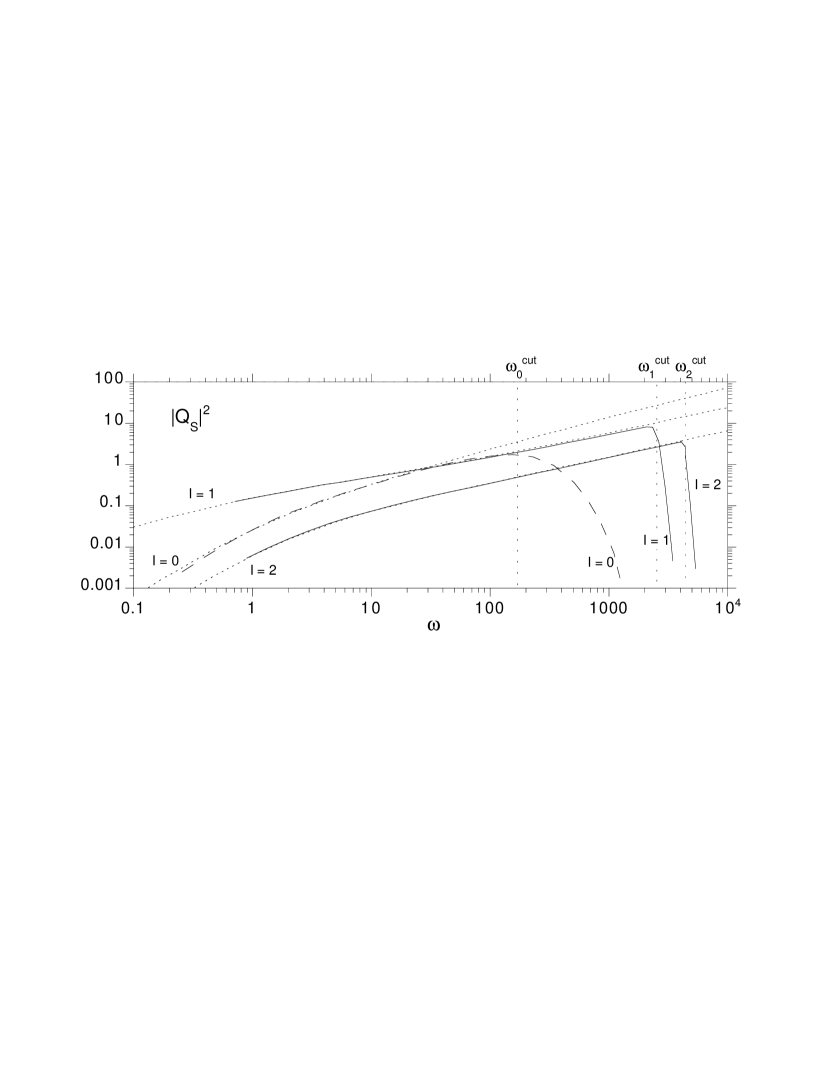
Figure 9: Acoustic efficiencies $|{\cal Q}_{S}|^{2}$ and $|{\cal Q}_{K}|^{2}$ depending on the frequency for $\gamma=1.665$ (i.e. $c_{\rm s}/c_{\infty}=20$), $l=0,1,2$. Frequencies are expressed in units of $c_{\infty}^{3}/GM$. These efficiencies are very close to those obtained for $\gamma=5/3$ (dotted lines), truncated after the cut-off frequency $\omega_{l}^{\rm cut}$.

For $\gamma$ close to $5/3$ and at frequencies lower than the cut off frequency, we can use the approximation of $|{\cal Q}_{S}|$ obtained for $\gamma=5/3$. According to Fig. 5, the maximum of $|{\cal Q}_{S}|$ is reached at the frequency $\omega_{l}^{\rm max}$, with $0.5<\omega_{l}^{\rm max}/\omega_{l}^{\rm cut}\leq 1$. The asymptotic behaviour of the maximum value of $|{\cal Q}_{S}|$ is therefore estimated by extrapolating Eqs. (28) and (29) to the cut-off frequency:

$${\rm Max}|{\cal Q}_{S}|_{l=0} \sim {1\over\gamma}\left({\omega_{0}^{\rm cut}\over 6}\right)^{1\over 3}\Gamma\left({2\over 3}\right),$$ (32)

$$\propto r_{\rm s}^{-{1\over 3}},$$ (33)

$${\rm Max}|{\cal Q}_{S}|_{l\geq 1} \sim {2^{1\over 2}\over 3\gamma}(\omega_{1}^{\rm cut})^{1\over 3}LK_{2\over 3}\left({2L\over 3}\right),$$ (34)

$$\propto LK_{2\over 3}\left({2L\over 3}\right)r_{\rm s}^{-{5\over 12}}.$$ (35)

It is interesting to note in Fig. 8 that the most efficient entropy perturbations at a given frequency when $\gamma<5/3$ are non radial ($l=1$), whereas radial ones are more efficient for $\gamma=5/3$ (Fig. 6). This is directly related to the fact that the critical refraction frequency is much higher for $l=1$ than for $l=0$ (Eqs. 19 and 21). This is illustrated in Fig. 9, where the acoustic efficiencies computed for $c_{\rm s}/c_{\infty}=20$ ($\gamma=1.665$) are very close to their values for $\gamma=5/3$, up to the refraction cut-off. In this figure, the efficiency $|{\cal Q}_{S}|$ is higher for $l=0$ than for $l=1$ in the limited range of frequencies $30<\omega<120$, but the overall maximum is reached near $\omega_{1}^{\rm cut}\sim 2300$ for $l=1$.

5 Conclusions

5.1 Summary

The acoustic response of the Bondi flow to pressure, entropy and vorticity perturbations has been studied thoroughly. Let us summarize the main results:

(i) the critical refraction frequency for acoustic waves $\omega_{l}^{\rm cut}$ is quite different from the ”natural” frequency $c_{\rm s}/r_{\rm s}$ one might think of at first glance. Moreover $\omega_{l}^{\rm cut}$ is also very different for radial and non radial perturbations. The two fundamental frequencies $\omega_{0}^{\rm cut},\omega_{1}^{\rm cut}$ of this flow near the sonic point were accurately determined (Eqs. 19 and 21), and are ordered as follows: $\omega_{0}^{\rm cut}<\omega_{1}^{\rm cut}<\omega_{K}$, with

$$\omega_{0}^{\rm cut} \propto {\rm Max}\left\{(1-{\cal M}^{2}){c\over r}\right\}\propto\left({\partial{\cal M}\over\partial\log r}\right)_{\rm s}{c_{\rm s}\over r_{\rm s}},$$ (36)

$$\omega_{1}^{\rm cut} \propto {\rm Max}\left\{(1-{\cal M}^{2})^{1\over 2}{c\over r}\right\}\propto\left({\partial{\cal M}\over\partial\log r}\right)_{\rm s}^{1\over 2}{c_{\rm s}\over r_{\rm s}}.$$ (37)

(ii) two quantities conserved in the linear approximation of the perturbed Bondi flow are source terms for acoustic waves: the entropy perturbation $\delta S$, and a quantity $\delta K$ related to both vorticity and entropy perturbations defined by Eq. (5).

(iii) the acoustic efficiencies ${\cal Q}_{S}$ and ${\cal Q}_{K}$ of entropy and vorticity perturbations are independent of the longitudinal number $m$.

(iv) $|{\cal Q}_{S}|$ and $|{\cal Q}_{K}|$ are highest for $l=1$ perturbations if $\gamma<5/3$.

(v) $|{\cal Q}_{K}|$ is highest at relatively low frequency, and is always rather moderate ($|{\cal Q}_{K}|<1$).

(vi) $|{\cal Q}_{S}|$ is highest at high frequency near the refraction cut-off, and can be much larger than one if $\gamma$ is close to $5/3$, i.e. if $c_{\rm s}/c_{\infty}\gg 1$. This confirms the physical argument of FT2000 which stressed the importance of the enthalpy increase between the outer part of the flow and the sonic point.

(vii) asymptotic scalings of $|{\cal Q}_{S}|,|{\cal Q}_{K}|$ were obtained at high frequency for $\gamma=5/3$ (Eqs. 28 to 30), in excellent agreement with numerical calculations.
The analytical expressions obtained for $\omega_{l}^{\rm cut}(\gamma)$, and for $|{\cal Q}_{S}|$ and $|{\cal Q}_{K}|$ at high frequency for $\gamma=5/3$, are accurate enough (see Figs. 3, 6 and 7) to be used as tests of the accuracy of 3D hydrodynamical codes used for Bondi accretion, and particularly their limitations at high frequency.

These results suggest that if a shock were present as outer boundary, the entropic-acoustic cycle would be unstable with respect to high frequency waves if the sound speed at the sonic point is high enough,i.e. if $\gamma$ is close to $5/3$. Indeed, an entropy perturbation $\delta S_{1}$ advected towards the accretor triggers an outgoing acoustic flux $F^{-}={\dot{M}}_{0}c^{2}|{\cal Q}_{S}|^{2}|\delta S|^{2}$. These acoustic waves propagate against the flow until they reach the shock, where they produce new entropy perturbations $\delta S_{2}$ (see FT2000), with $\delta S_{2}>\delta S_{1}$ since $|{\cal Q}_{S}|\gg 1$. The eigenmodes corresponding to this unstable cycle will be investigated in the second paper of this series (Foglizzo 2001). The fact that the most unstable simulations of Bondi-Hoyle-Lyttleton accretion also correspond to $\gamma=5/3$ (Ruffert & Arnett 1994, Ruffert 1994b) already encourages us to look for an extrapolation of these results to the case of non-radial shocked accretion flows.

5.2 Discussion

5.2.1 Upper bound for $|{\cal Q}_{S}|^{2}$ imposed by the Schwarzschild radius

In the flow $\gamma=5/3$, the fact that the outgoing acoustic flux produced by entropy perturbations diverges at high frequency (Eqs. 28 and 29) is rather surprising, and directly related to the hypothesis of a point-like newtonian accretor ($r_{\rm s}=0$). In this section we show that $|{\cal Q}_{S}|^{2}$ is naturally bounded if the finite size of the accretor is taken into account. Simple arguments are used in order to roughly estimate this upper bound in the case of an accreting black hole, without computing the exact relativistic corrections near its horizon.
Let us denote by $r_{\rm Sch}=2GM/c_{\rm light}^{2}$ the Schwarzschild radius of the black hole, where $c_{\rm light}$ is the speed of light. With a sound speed at infinity $c_{\infty}\ll c_{\rm light}$, Eq. (1) guarantees that relativistic effects are negligible except for $\gamma$ close to $5/3$. Indeed Petrich et al. (1989) checked numerically that relativistic corrections are small for $\gamma=1.1$ and $\gamma=4/3$. If $\gamma=5/3$, the sonic point is bound to lie at a few Schwarzschild radii:

$$\eta\equiv{r_{\rm s}\over r_{\rm Sch}}>1.$$ (38)

Our description of non radial acoustic waves in the flow $\gamma=5/3$ is not affected by relativistic corrections as long as their turning point $r_{t}$ is far enough from the horizon. Since $r_{t}\sim(L/\omega)^{4/5}$ at high frequency (Eq. 122), a natural relativistic cut-off is introduced for $r_{t}\sim\eta r_{\rm Sch}$:

$$\omega_{l\geq 1}^{\rm cut}\sim{0.25\over\eta^{5\over 4}}\left[{l(l+1)\over 2}\right]^{1\over 2}\left({c_{\infty}\over c_{\rm light}}\right)^{1\over 2}{c^{3}\over GM}.$$ (39)

The efficiency $|{\cal Q}_{S}|^{2}$ of the generation of non radial acoustic waves close to this cut-off frequency is deduced from Eq. (29):

$$|{\cal Q}_{S}|^{2}\sim{0.1\over\eta^{5\over 6}}\left({L^{2}\over 2}\right)^{7\over 6}{\rm e}^{-{4L\over 3}}\left({c_{\rm light}\over c_{\infty}}\right)^{5\over 3}.$$ (40)

The numerical values of the cut-off frequency and maximum acoustic efficiency of the entropy perturbations $l=1$ are thus typically:

$$\omega_{1}^{\rm cut} \sim {100\over\eta^{5\over 4}}\left({c_{\infty}\over 100\;{\rm km/s}}\right)^{1\over 2}\left({M\over 10M_{\rm sol}}\right)^{-1}\;{\rm Hz},$$ (41)

$$|{\cal Q}_{S}|^{2}_{\rm max} \sim {10^{4}\over\eta^{5\over 6}}\left({c_{\infty}\over 100\;{\rm km/s}}\right)^{-{5\over 3}}.$$ (42)

Therefore relativistic effects set an upper bound on the apparent divergence of $|{\cal Q}_{S}|$ at high frequency for $\gamma=5/3$. Eq. (42) indicates that entropy perturbations may excite low degree acoustic waves very efficiently, up to non linear amplitudes if the component $l=1$ of the entropy perturbations exceeds a few percent. This efficiency is much smaller for inhomogeneities with a small angular scale, since $|{\cal Q}_{S}|$ decreases exponentially when $l$ increases (Eq. 40).

5.2.2 Non adiabatic limitations

Non adiabatic processes are discussed by Chang & Ostriker (1985) in the context of Bondi accretion. The efficiency $|{\cal Q}_{S}|$ would be strongly affected by a strong thermal conduction which smoothes out entropy perturbations. This effect would be more pronounced for short wavelength perturbations, which are also the most efficient for $\gamma$ close to $5/3$. Without going into the details of such processes, our understanding of the acoustic efficiency allows the following remark: if the inner region of the flow were dominated by non adiabatic processes, the optimal frequency for $|{\cal Q}_{S}|$ would be at most reduced to the maximum frequency of acoustic waves refracted inside the adiabatic region of the flow. Even when there is no shock, the mechanism of excitation of acoustic waves from the advection of entropy perturbations opens interesting perspectives to the problem of time delay in Cygnus X-1, approached numerically by Manmoto et al. (1996). Interpreting their results in terms of acoustic efficiency of entropy perturbations suggest that this physical process survives the inclusion of rotation, radiative cooling and viscous heating. The study of effects deserve a careful analysis which is beyond the scope of the present paper.

Appendix A Description of the unperturbed Bondi flow

A.1 $\gamma<5/3$

The Bernoulli equation and the conservation of mass are written after normalizing velocities to the sound speed $c_{\infty}$ at infinity, and distances to the Bondi radius $GM/c_{\infty}^{2}$

$${v^{2}\over 2}+{c^{2}-1\over\gamma-1} = {1\over r},$$ (43)

$$-r^{2}vc^{2\over\gamma-1} = \left({1\over 2}\right)^{\gamma+1\over 2(\gamma-1)}\left({4\over 5-3\gamma}\right)^{5-3\gamma\over 2(\gamma-1)}.$$ (44)

By taking the radial derivative of these equation, we obtain:

$${\partial\log c\over\partial\log r} = {\gamma-1\over 2}{{\cal M}^{2}\over 1-{\cal M}^{2}}\left(2-{1\over rv^{2}}\right),$$ (45)

$${\partial\log v\over\partial\log r} = {1\over 1-{\cal M}^{2}}\left({1\over rc^{2}}-2\right).$$ (46)

At the sonic point, $r_{\rm s},c_{\rm s}$ are defined by Eqs. (1) and 2). A Taylor expansion of Eqs. (45) and (46) leads to:

$${\partial\log v\over\partial\log r}(r_{\rm s}) = -{2\over\gamma+1}\left[\gamma-1+\left({5-3\gamma\over 2}\right)^{1\over 2}\right],$$ (47)

$${\partial\log c\over\partial\log r}(r_{\rm s}) = -{\gamma-1\over\gamma+1}\left[2-\left({5-3\gamma\over 2}\right)^{1\over 2}\right],$$ (48)

$${\partial\log{\cal M}\over\partial\log r}(r_{\rm s}) = -\left({5-3\gamma\over 2}\right)^{1\over 2}.$$ (49)

A.2 $\gamma=5/3$

In accretion flows where $\gamma=5/3$, Eqs. (43) and (44) become:

$${v^{2}\over 2}+{3\over 2}(c^{2}-1) = {1\over r},$$ (50)

$$r^{2}vc^{3} = -{1\over 4}.$$ (51)

$r,v,c$ can be expressed as explicit functions of the variable $x$ defined by:

$$x \equiv {1\over{\cal M}^{1\over 2}},$$ (52)

$${\partial r\over\partial x} = {1-{\cal M}^{2}\over 2},$$ (53)

$$r = {(x-1)^{2}(9x^{4}+2x^{2}+1)\over 6x^{3}(3x^{2}-2x+1)},$$ (54)

$$v^{2} = {3\over(x-1)^{2}}{3x^{2}-2x+1\over 9x^{4}+2x^{2}+1},$$ (55)

$$c^{2} = {3x^{4}\over(x-1)^{2}}{3x^{2}-2x+1\over 9x^{4}+2x^{2}+1}.$$ (56)

Appendix B Linearized equations for perturbations

B.1 Second order differential system

The Euler equation is written as follows:

$${\partial v\over\partial t}+w\times v+\nabla\left({v^{2}\over 2}+{c^{2}\over\gamma-1}-{GM\over r}\right)=c^{2}\nabla{S\over\gamma}.$$ (57)

Projecting the Euler equation onto the flow velocity, we obtain the equation of evolution of the Bernoulli constant:

$$\left({\partial\over\partial t}+v\cdot\nabla\right)\left({v^{2}\over 2}+{c^{2}\over\gamma-1}-{GM\over r}\right)={1\over\rho}{\partial p\over\partial t}.$$ (58)

By combining the curl of Euler equation and the mass conservation, we obtain the equation for the evolution of the vorticity $w$:

$${\partial\over\partial t}{w\over\rho}+({v\cdot\nabla}){w\over\rho}=\left({w\over\rho}\cdot\nabla\right)v+{1\over\rho}\nabla c^{2}\times\nabla{S\over\gamma}.$$ (59)

We make a Fourier transform in time of the linearized equations describing the radial flow perturbed in spherical coordinated $(r,\theta,\varphi)$. The linearized equation of entropy conservation can be directly integrated:

$$\delta S=\delta S_{R}{\rm e}^{i\omega\int_{R}^{r}{{\rm d}r\over v}}.$$ (60)

The vorticity equation (59) can also be integrated when linearized:

$$w_{r} = \left({R\over r}\right)^{2}(w_{r})_{R}{\rm e}^{i\omega\int_{R}^{r}{{\rm d}r\over v}},$$ (61)

$$w_{\theta} = {1\over rv}\left[Rv_{R}(w_{\theta})_{R}-{c^{2}-c_{R}^{2}\over\sin\theta}{\partial\over\partial\varphi}{\delta S_{R}\over\gamma}\right]{\rm e}^{i\omega\int_{R}^{r}{{\rm d}r\over v}},$$ (62)

$$w_{\varphi} = {1\over rv}\left[Rv_{R}(w_{\varphi})_{R}+(c^{2}-c_{R}^{2}){\partial\over\partial\theta}{\delta S_{R}\over\gamma}\right]{\rm e}^{i\omega\int_{R}^{r}{{\rm d}r\over v}}.$$ (63)

Thus the product $r^{2}w_{r}$ is conserved during advection, as remarked by Kovalenko & Eremin (1998). In order to write the linearized Euler equation in the simplest form, let us define the two functions $f,g$ as follows:

$$f \equiv v\;\delta v_{r}+{2\over\gamma-1}c\;\delta c,$$ (64)

$$g \equiv {\delta v_{r}\over v}+{2\over\gamma-1}{\delta c\over c}.$$ (65)

$f$ is the perturbation of the Bernoulli constant, which is directly related to the pressure variations according to Eq. (58). $g$ is related to the perturbation of the mass accretion rate and entropy through:

$$g={\delta\dot{M}\over\dot{M}}+\delta S.$$ (66)

By linearization of Eq. (57), we express the velocity components $(\delta v_{\theta},\delta v_{\varphi})$ as follows:

$${\delta v_{\theta}\over v} = {w_{\varphi}\over i\omega}+{1\over i\omega rv}{\partial\over\partial\theta}f-{c^{2}\over i\omega rv}{\partial\over\partial\theta}{\delta S_{R}\over\gamma}{\rm e}^{i\omega\int_{R}^{r}{{\rm d}r\over v}},$$ (67)

$${\delta v_{\varphi}\over v} = -{w_{\theta}\over i\omega}+{1\over i\omega rv\sin\theta}\left[{\partial\over\partial\varphi}f-c^{2}{\partial\over\partial\varphi}{\delta S_{R}\over\gamma}{\rm e}^{i\omega\int_{R}^{r}{{\rm d}r\over v}}\right].$$ (68)

The radial part of the Euler equation, together with the continuity equation, lead to the following differential system:

$$v{\partial f\over\partial r}+{i\omega{\cal M}^{2}f\over 1-{\cal M}^{2}} = {i\omega v^{2}g\over 1-{\cal M}^{2}}+i\omega c^{2}{\delta S_{R}\over\gamma}{\rm e}^{i\omega\int_{R}^{r}{{\rm d}r\over v}},$$ (69)

$$v{\partial g\over\partial r}+{i\omega{\cal M}^{2}g\over 1-{\cal M}^{2}} = {i\omega f\over c^{2}(1-{\cal M}^{2})}+{i\over\omega}\Delta_{\theta,\varphi}f+{i\delta K_{R}\over r^{2}\omega}{\rm e}^{i\omega\int_{R}^{r}{{\rm d}r\over v}},$$

where $\Delta_{\theta,\varphi}$ is the non radial part of the Laplacian in spherical coordinates. The constant $\delta K_{R}$ is defined as follows:

$$\delta K\equiv r^{2}\left[v\cdot(\nabla\times w)-c^{2}\Delta_{\theta,\varphi}{\delta S\over\gamma}\right].$$ (71)

We deduce from Eqs. (62-63) that $\delta K$ is conserved when advected:

$$\left\{{\partial\over\partial t}+v{\partial\over\partial r}\right\}\delta K=0.$$ (72)

$\delta K$ can be written independently of the system of coordinates, as the first order perturbation of the quantity $K$ defined by:

$$K\equiv{{\dot{M}}\over 4\pi}{{\bf v}\over\rho v}.\left[\nabla\times{\bf w}-c^{2}\nabla\times\left({{\bf v}\over v^{2}}\times\nabla{S\over\gamma}\right)\right],$$ (73)

but the conservation of $K$ is established only in the linear approximation. By projecting $f,g,\delta S_{R}$ and the radial component of the curl of the vorticity $(\nabla\times w_{R})_{r}$ onto the spherical harmonics $Y_{l}^{m}(\theta,\varphi)$, which are the eigenvectors of the Laplacian, we obtain:

$$v{\partial f\over\partial r}+{i\omega{\cal M}^{2}f\over 1-{\cal M}^{2}} = {i\omega v^{2}g\over 1-{\cal M}^{2}}+i\omega c^{2}{\delta S_{R}\over\gamma}{\rm e}^{i\omega\int_{R}^{r}{{\rm d}r\over v}},$$ (74)

$$v{\partial g\over\partial r}+{i\omega{\cal M}^{2}g\over 1-{\cal M}^{2}} = {i\omega f\over c^{2}(1-{\cal M}^{2})}-{iL^{2}\over\omega r^{2}}f+{i\delta K_{R}\over r^{2}\omega}{\rm e}^{i\omega\int_{R}^{r}{{\rm d}r\over v}},$$ (75)

where we have defined $L^{2}\equiv l(l+1)$ for the sake of the simplicity of the equations.

B.2 Second order differential equation

B.2.1 Pressure perturbation

The most natural function to describe the behaviour of acoustic waves is the pressure perturbation $\delta p/p$, which is related to the sound speed perturbation through:

$${\delta p\over\gamma p}={2\over\gamma-1}{\delta c\over c}-{\delta S_{R}\over\gamma}{\rm e}^{i\omega\int_{R}^{r}{{\rm d}r\over v}}.$$ (76)

Using this equation in Eqs. (64-65) enables us to write $(f,g)$ as functions of $\delta v_{r}$ and $\delta p$ in Eqs. (74-75), and thus obtain Eq. (4) with:

$$a_{1} \equiv {\partial\log\over\partial r}{(c^{2}-v^{2})^{2}\over v\Delta}+{2i\omega v\over c^{2}-v^{2}},$$ (77)

$$a_{0} \equiv {1\over c^{2}-v^{2}}\left\{\omega^{2}-L^{2}{c^{2}\over r^{2}}-{1\over v}{\partial\over\partial r}\left({c^{4}\over v}{\partial{\cal M}^{2}\over\partial r}\right)+\right.$$ (78)

$$\left.2i\omega{\partial v\over\partial r}+c^{2}{\partial\log\Delta\over\partial r}\left[{\partial\log{\cal M}^{2}\over\partial r}-(1+{\cal M}^{2}){i\omega\over v}\right]\right\},$$

$$b_{0} \equiv {-i\Delta\over vc^{2}(1-{\cal M}^{2})}{\rm e}^{i\omega\int_{R}^{r}{{\rm d}r\over v}}{\partial\over\partial r}\left[{c^{2}\over\Delta}\left(\omega-iv{\partial\log\over\partial r}{1\over{\cal M}^{2}}\right)\right],$$ (79)

$$b_{1} \equiv -{i\gamma\Delta\over vc^{2}(1-{\cal M}^{2})}{\rm e}^{i\omega\int_{R}^{r}{{\rm d}r\over v}}{\partial\over\partial r}{v^{2}\over\omega r^{2}\Delta},$$ (80)

$$\Delta \equiv \omega^{2}+2i\omega{\partial v\over\partial r}+L^{2}{v^{2}\over r^{2}}.$$ (81)

The function $\Delta$ is introduced by our choice of writing the differential equation satisfied by the pressure perturbation, which is justified from the physical point of view. Note that $\Delta$ never vanishes as long as the real part of the frequency is different from zero.

B.2.2 A more compact mathematical formulation

It is convenient to define ($\tilde{f},\tilde{g}$) as:

$${\tilde{f}} \equiv {\rm e}^{i\omega\int_{R}^{r}{{\cal M}^{2}\over 1-{\cal M}^{2}}{{\rm d}r\over v}}f,$$ (82)

$${\tilde{g}} \equiv {\rm e}^{i\omega\int_{R}^{r}{{\cal M}^{2}\over 1-{\cal M}^{2}}{{\rm d}r\over v}}g.$$ (83)

The differential system Eqs. (74-75) is then simpler:

$${\partial\tilde{f}\over\partial r} = {i\omega v{\tilde{g}}\over 1-{\cal M}^{2}}+i\omega{c^{2}\over v}{\delta S_{R}\over\gamma}{\rm e}^{i\omega\int_{R}^{r}{{\rm d}r\over v(1-{\cal M}^{2})}},$$ (84)

$${\partial\tilde{g}\over\partial r} = {i{\tilde{f}}\over\omega v}\left[{\omega^{2}\over c^{2}(1-{\cal M}^{2})}-{L^{2}\over r^{2}}\right]+{i\delta K_{R}\over r^{2}\omega v}{\rm e}^{i\omega\int_{R}^{r}{{\rm d}r\over v(1-{\cal M}^{2})}}.$$ (85)

The homogeneous differential equation ( 9) can be transformed into a more compact form using the new variable $X$:

$${{\rm d}X\over{\rm d}r} \equiv {v\over 1-{\cal M}^{2}},$$ (86)

$$W \equiv {1\over v^{2}c^{2}}(\omega^{2}-\omega_{l}^{2}),$$ (87)

where $\omega_{l}$ is defined by Eq. (7).

$${\partial^{2}\tilde{f}\over\partial X^{2}}+W\tilde{f}=$$

$$-{1-{\cal M}^{2}\over v}{\rm e}^{i\omega\int{{\rm d}X\over v^{2}}}\left\{{\omega\over{\cal M}^{2}}{\delta S_{R}\over\gamma}\left({\omega\over v}+i{\partial\log{\cal M}^{2}\over\partial r}\right)+{\delta K_{R}\over vr^{2}}\right\}.$$

(88)

With this new variable, the sonic point $r_{\rm s}$ corresponds to $X\to+\infty$, while the spatial infinity corresponds to $X=0$.

Appendix C Approximations of the homogeneous solution

C.1 WKB approximation far from the accretor

The general solution $f$ of the homogeneous equation associated to Eq. (88) is a linear combination of ingoing ($f_{+}$) and outgoing ($f_{-}$) waves, which can be approximated by the WKB method:

$${\tilde{f}^{\pm}}\sim{\omega^{1\over 2}\over W^{1\over 4}}\exp\left(\pm i\int^{r}{vW^{1\over 2}\over 1-{\cal M}^{2}}{\rm d}r\right).$$ (89)

This approximation is asymptotically valid for

$${\partial\log W\over\partial X}\ll W^{1\over 2},$$ (90)

which is satisfied at high frequency or far from the accretor. The Wronskien ${\cal W}$ associated to the couple (${\tilde{f}^{+}},{\tilde{f}^{-}}$) of solutions is:

$${\cal W} \equiv {\tilde{f}^{+}}{\partial{\tilde{f}^{-}}\over\partial r}-{\tilde{f}^{-}}{\partial{\tilde{f}^{+}}\over\partial r},$$ (91)

$$= -{2i\omega v\over 1-{\cal M}^{2}}.$$ (92)

The pressure perturbation $\Delta p$ associated to a perturbation $f$ is deduced from Eq. (58):

$${\Delta p\over\gamma p}={1\over c^{2}}{\rm e}^{-i\omega\int^{r}{{\cal M}^{2}\over 1-{\cal M}^{2}}{{\rm d}r\over v}}\left({{\tilde{f}}\over 1-{\cal M}^{2}}+{iv\over\omega}{\partial{\tilde{f}}\over\partial r}\right).$$ (93)

The normalization factor $\omega^{1\over 2}$ in Eq. (89) is such that the pressure perturbations $\Delta p_{\pm}$ associated to these solutions by Eq. (58) have the following asymptotic behaviour:

$${\Delta p^{\pm}\over\gamma p}\sim{c_{\infty}\over c}{{\cal M}^{1\over 2}\over 1\pm{\cal M}}{\rm e}^{\mp i\omega{r\over c_{\infty}}}.$$ (94)

Both carry the same acoustic flux $F^{\pm}={\dot{M}}_{0}c_{\infty}^{2}$ according to Eq. (10).

C.2 Definition of the refraction coefficient ${\bar{\cal R}_{s}}$ and estimate at high frequency

C.2.1 $\gamma<5/3$

A Frobenius expansion in the vicinity of the sonic point (${\cal M}=1$) shows that any solution of the homogeneous equation can be projected onto the couple $f_{1},f_{2}$ of solutions, where $f_{1}(r)$ is regular and $f_{2}(r)$ is singular:

$$f_{1}(r) \sim 1+{\cal O}(r),$$ (95)

$$f_{2}(r) \sim \left[1+{\cal O}(r)\right]\exp\left\{{i\omega\over 2c_{\rm s}{\dot{\cal M}}_{\rm s}}\log(r-r_{\rm s})\right\}.$$ (96)

This defines a unique coefficient ${\bar{\cal R}_{s}}$ such that the solution

$$f_{0}\equiv f^{+}+{\bar{\cal R}_{s}}f^{-},$$ (97)

is regular at the sonic point. The coefficient $|{\bar{\cal R}_{s}}|^{2}$ is the refraction coefficient of sound waves. The linearity of the equations guarantees of course that the solution $\Delta p_{0}\equiv\Delta p^{+}+{\bar{\cal R}_{s}}\Delta p^{-}$ is also regular.
An expansion of $W$ in the vicinity of the sonic point leads to:

$$W = q_{0}+q_{1}(r-r_{\rm s})+{\cal O}(r-r_{\rm s})^{2},$$ (98)

$$q_{0} \equiv {\omega^{2}\over c_{\rm s}^{4}},$$ (99)

$$q_{1} \equiv -{\omega^{2}\over c_{\rm s}^{4}}{\partial\log c^{2}v^{2}\over\partial r}+{2L^{2}{\dot{\cal M}}_{\rm s}\over c_{\rm s}^{2}r_{\rm s}^{2}},$$ (100)

$$r-r_{\rm s} \sim \exp\left({2{\dot{\cal M}}_{\rm s}\over c_{\rm s}}X\right).$$ (101)

The WKB approximation of ${\tilde{f}}^{\pm}$ is valid at high frequency $\omega\gg\omega_{l}^{\rm cut}$, for $r-r_{\rm s}\ll 1$:

$${\tilde{f}}^{\pm}\sim c_{\rm s}\exp\pm i\left[{\omega\over 2c_{\rm s}{\dot{\cal M}}_{\rm s}}\log(r-r_{\rm s})+{\cal O}(1)\right].$$ (102)

The asymptotic solution to the differential equation (9) can also be approximated by a Bessel function in the vicinity of the sonic point, for $r-r_{\rm s}\ll 1$. The regularity of $f_{0}$ at the sonic radius implies:

$${\tilde{f}_{0}} \sim \lambda J_{\nu}\left[{-c_{\rm s}q_{1}^{1\over 2}\over{\dot{\cal M}}_{\rm s}}(r-r_{\rm s})^{1\over 2}\right],$$ (103)

$$\nu \equiv {ic_{\rm s}q_{0}^{1\over 2}\over{\dot{\cal M}}_{\rm s}}={i\omega\over c_{\rm s}{\dot{\cal M}}_{\rm s}}.$$ (104)

The Bessel and WKB approximations are both valid in the region where $\omega^{-1}\ll r-r_{\rm s}\ll 1$. In this region, the matching of the two approximations gives the normalization constant $\lambda$ and the refraction coefficient ${\bar{\cal R}_{s}}$. The asymptotic behavior of the Bessel function, when both the imaginary order $\nu$ and the argument tend to infinity, is obtained from Watson (1952, Chap. 8.6, p.262). The Bessel function $J_{\nu}(z)$ is written in terms of the Hankel functions $H_{\nu}^{(1)}(z)$ and $H_{\nu}^{(2)}(z)$. Let $x,z$ be real numbers, with $|x|,z\gg 1$, such that the order $\nu$ is purely imaginary $\nu\equiv iz\sinh x$:

$$J_{\nu}(z) = {1\over 2}\left[H_{\nu}^{(1)}(z)+H_{\nu}^{(2)}(z)\right],$$ (105)

$$H_{\nu}^{(1)}(z) \sim \left[{2\exp(\pi z\sinh x)\over\pi z\cosh x}\right]^{1\over 2}{\rm e}^{+i\left[z(\cosh x-x\sinh x)-{\pi\over 4}\right]},$$ (106)

$$H_{\nu}^{(2)}(z) \sim \left[{2\exp(-\pi z\sinh x)\over\pi z\cosh x}\right]^{1\over 2}{\rm e}^{-i\left[z(\cosh x-x\sinh x)-{\pi\over 4}\right]}.$$ (107)

Applying these asymptotic expansions to Eq. (103), with

$$z \equiv -{c_{\rm s}q_{1}^{1\over 2}\over{\dot{\cal M}}_{\rm s}}(r-r_{\rm s})^{1\over 2}>0,$$ (108)

$$\sinh x = {\nu\over iz}\sim-\left|(r-r_{\rm s}){\partial\log c^{2}v^{2}\over\partial r}\right|^{-{1\over 2}}<0,$$ (109)

we obtain $\lambda$ and $|f_{0}(r_{\rm s})|$ to first order at high frequency:

$$\lambda = \left|{2\pi c_{\rm s}\omega\over{\dot{\cal M}}_{\rm s}}\right|^{1\over 2}{\rm e}^{\omega\pi\over 2c_{\rm s}{\dot{\cal M}}_{\rm s}},$$ (110)

$$|f_{0}(r_{\rm s})| = c_{\rm s}.$$ (111)

The exponential decrease of $|{\bar{\cal R}_{s}}|$ at high frequency is deduced from Eqs. (106) and (107), by identifying the Hankel functions with the ingoing and outgoing acoustic waves:

$$|{\bar{\cal R}_{s}}|\propto{\rm e}^{\omega\pi\over c_{\rm s}{\dot{\cal M}}_{\rm s}}.$$ (112)

C.2.2 $\gamma=5/3$, $l=0$

The WKB approximation is valid in the range $r\gg 1/\omega$.

$$\tilde{f}^{\pm}\sim c{\cal M}^{1\over 2}\exp\pm i\omega\int_{0}^{r}{{\cal M}\over v(1-{\cal M}^{2})}{\rm d}r,$$ (113)

where the normalization is chosen in agreement with Eq. (89). In the region $r\leq 1/\omega$ where the WKB approximation is not valid, we approximate the solution by the Bessel function $J_{0}$, which is regular at the origin:

$${\partial^{2}\tilde{f}_{0}\over\partial r^{2}} + {1\over r}\left[1+{\cal O}(r^{1\over 2})\right]{\partial\tilde{f}_{0}\over\partial r}+{\omega^{2}\over 8}\tilde{f}_{0}\left[1+{\cal O}(r^{1\over 2})\right]=0,$$ (114)

$$\tilde{f}_{0} \sim \tilde{f}_{0}(0)J_{0}\left({\omega r\over 2^{3\over 2}}\right).$$ (115)

The other Bessel solution, $Y_{0}$, is singular with a logarithmic divergence, as in the case of $\gamma<5/3$. The Bessel approximation for $r\gg 1/\omega$ matches the WKB approximation:

$$\tilde{f}_{0}(0)J_{0}\left({\omega r\over 2^{3\over 2}}\right) \sim \tilde{f}_{0}(0)\left({2^{5\over 2}\over\pi\omega r}\right)^{1\over 2}\cos\left({\omega r\over 2^{3\over 2}}-{\pi\over 4}\right),$$ (116)

$$\sim {1\over 2^{1\over 2}\gamma r^{1\over 2}}\left({\rm e}^{-i{\omega r\over 2^{3\over 2}}}+{\bar{\cal R}_{s}}{\rm e}^{+i{\omega r\over 2^{3\over 2}}}\right).$$ (117)

From this we deduce that:

$$\tilde{f}_{0}(0) = {\cal O}\left(\omega^{1\over 2}\right),$$ (118)

$$|{\bar{\cal R}_{s}}| = 1.$$ (119)

C.2.3 $\gamma=5/3$, $l\geq 1$

The case of non radial perturbations needs to be treated separately, because the behaviour of the solution is quite different near the sonic point. If $l\geq 1$, there is always a turning point beyond which the solution is evanescent, such that it decays exponentially on the sonic point. The leading behaviour of $f_{0},g_{0}$ on this essential singularity is the following, within a multiplicative constant:

$$f_{0} \sim r^{1\over 8}\exp-{2L\over r^{1\over 4}},$$ (120)

$$g_{0} \sim 2^{3\over 2}{iL\over\omega r^{1\over 8}}\exp-{2L\over r^{1\over 4}}.$$ (121)

The solutions of the other branch diverge exponentially on the sonic point: as in the case of a regular sonic point, there is a unique combination of ingoing and outgoing waves such that the solution does not diverge at the sonic point. The turning point $r_{\rm t}$ corresponds to the radius where $W=0$ in Eq. (88):

$$r_{\rm t}\sim\left({2L^{2}\over\omega^{2}}\right)^{2\over 5}.$$ (122)

The WKB approximation is valid for $r_{\rm t}\ll r\ll 1$:

$$\tilde{f}_{\pm} \sim {c{\cal M}^{1\over 2}\over\left[1-{L^{2}c^{2}\over r^{2}\omega^{2}}(1-{\cal M}^{2})\right]^{1\over 4}}\times$$ (123)

$$\exp\pm i\omega\int_{r_{0}}^{r}{{\cal M}\over v(1-{\cal M}^{2})}\left[1-{L^{2}c^{2}\over r^{2}\omega^{2}}(1-{\cal M}^{2})\right]^{1\over 2}{\rm d}r.$$

Appendix D Acoustic efficiencies ${\cal Q}_{S},{\cal Q}_{K}$ of entropy and vorticity perturbations

D.1 Acoustic efficiency ${\cal Q}_{K}$

The outgoing pressure perturbation produced by the advection of a perturbation $\delta K_{R}$ is computed by solving Eq. (88), imposing the regularity at the sonic point and the absence of an incoming sound wave from infinity. The general solution of Eq. (88) with $\delta S_{R}=0$ can be written as:

$${\tilde{f}} = -{i\delta K_{R}\over 2\omega}\left[{\tilde{f}^{-}}\left\{\beta+\int_{r_{0}}^{r}{{\tilde{f}^{+}}\over r^{2}v}{\rm e}^{i\omega\int^{r}{{\rm d}r\over v(1-{\cal M}^{2})}}\right\}-\right.$$ (124)

$$\left.{\tilde{f}^{+}}\left\{\alpha+\int_{r_{0}}^{r}{{\tilde{f}^{-}}\over r^{2}v}{\rm e}^{i\omega\int^{r}{{\rm d}r\over v(1-{\cal M}^{2})}}\right\}\right],$$

$${\delta p\over\gamma p} = -{i\delta K_{R}\over 2\omega}\left[{\Delta p^{-}\over\gamma p}\left\{\beta+\int_{r_{0}}^{r}{{\tilde{f}^{+}}\over r^{2}v}{\rm e}^{i\omega\int^{r}{{\rm d}r\over v(1-{\cal M}^{2})}}\right\}-\right.$$ (125)

$$\left.{\Delta p^{+}\over\gamma p}\left\{\alpha+\int_{r_{0}}^{r}{{\tilde{f}^{-}}\over r^{2}v}{\rm e}^{i\omega\int^{r}{{\rm d}r\over v(1-{\cal M}^{2})}}\right\}\right].$$

According to Eqs. (94) and (95-96), the integrals involved in Eq. (125) are well defined both at infinity and at the sonic radius. The condition that no sound wave comes from infinity leads to:

$$\alpha=-\int_{r_{0}}^{\infty}{{\tilde{f}^{-}}\over r^{2}v}{\rm e}^{i\omega\int^{r}{{\rm d}r\over v(1-{\cal M}^{2})}}.$$ (126)

The regularity at the sonic radius can be written:

$$\beta=-{\bar{\cal R}_{s}}\alpha-\int_{r_{0}}^{r_{\rm s}}{{\tilde{f}_{0}}\over r^{2}v}{\rm e}^{i\omega\int^{r}{{\rm d}r\over v(1-{\cal M}^{2})}}.$$ (127)

Thus the efficiency of sound wave emission by the advection of vorticity perturbations is:

$${\cal Q}_{K}=-{i\over 2\omega}\int_{r_{\rm s}}^{\infty}{\rm e}^{i\omega\int_{R}^{r}{1+{\cal M}^{2}\over 1-{\cal M}^{2}}{{\rm d}r\over v}}{f_{0}\over r^{2}v}{\rm d}r.$$ (128)

This integral converges as $1/r^{3}$ at infinity. It can be transformed using integrations by parts together with the homogeneous differential system satisfied by $f_{0},g_{0}$, so that it converges rapidly at infinity, thus allowing an easier numerical computation. The following expression converges as $1/r^{5}$:

$${\cal Q}_{K}={1\over 2\omega^{2}} \int_{r_{\rm s}}^{\infty}{\rm e}^{i\omega\int_{R}^{r}{1+{\cal M}^{2}\over 1-{\cal M}^{2}}{{\rm d}r\over v}}$$ (129)

$$\times\left\{{\partial\over\partial r}\left({1-{\cal M}^{2}\over r^{2}}\right)f_{0}+{i\omega v\over r^{2}}g_{0}\right\}{\rm d}r.$$

D.2 Acoustic efficiency ${\cal Q}_{S}$

The outgoing pressure perturbation produced by an incoming entropy perturbation $\delta S_{R}$ is also computed by solving Eq. (88), imposing the regularity at the sonic point and the absence of an incoming sound wave from infinity. The general solution of Eq. (88) with $\delta K_{R}=0$ can be written as:

$${\tilde{f}}=-{\delta S_{R}\over 2\gamma}\times$$

$$\left[{\tilde{f}^{-}}\left\{\beta+\int_{r_{0}}^{r}{\tilde{f}^{+}}{\partial\over\partial r}\left({1-{\cal M}^{2}\over{\cal M}^{2}}{\rm e}^{i\omega\int^{r}{{\rm d}r\over v(1-{\cal M}^{2})}}\right)\right\}-\right.$$

$$\left.{\tilde{f}^{+}}\left\{\alpha+\int_{r_{0}}^{r}{\tilde{f}^{-}}{\partial\over\partial r}\left({1-{\cal M}^{2}\over{\cal M}^{2}}{\rm e}^{i\omega\int^{r}{{\rm d}r\over v(1-{\cal M}^{2})}}\right)\right\}\right],$$ (130)

$${\delta p\over\gamma p}=-{\delta S_{R}\over 2\gamma}\times$$

$$\left[{\Delta p^{-}\over\gamma p}\left\{\beta+\int_{r_{0}}^{r}{\tilde{f}^{+}}{\partial\over\partial r}\left({1-{\cal M}^{2}\over{\cal M}^{2}}{\rm e}^{i\omega\int^{r}{{\rm d}r\over v(1-{\cal M}^{2})}}\right)\right\}-\right.$$

$$\left.{\Delta p^{+}\over\gamma p}\left\{\alpha+\int_{r_{0}}^{r}{\tilde{f}^{-}}{\partial\over\partial r}\left({1-{\cal M}^{2}\over{\cal M}^{2}}{\rm e}^{i\omega\int^{r}{{\rm d}r\over v(1-{\cal M}^{2})}}\right)\right\}\right].$$ (131)

Since the integrals of Eq. (131) converge at the sonic point, the regularity of the solution at the sonic point can be written:

$$\beta=-\alpha{\bar{\cal R}_{s}}-\int_{r_{0}}^{r}{\tilde{f}_{0}}{\partial\over\partial r}\left({1-{\cal M}^{2}\over{\cal M}^{2}}{\rm e}^{i\omega\int^{r}{{\rm d}r\over v(1-{\cal M}^{2})}}\right).$$ (132)

In Eq. (131) the integrals diverge at infinity. Two integrations by parts leads to define the two functions $F_{\pm},H_{\pm}$ as follows:

$$F^{\pm} \equiv c^{2}{(1-{\cal M}^{2})^{2}\over{\cal M}^{2}}{\Delta p^{\pm}\over\gamma p}{\rm e}^{i\omega\int^{r}{1+{\cal M}^{2}\over 1-{\cal M}^{2}}{{\rm d}r\over v}},$$ (133)

$$H^{\pm} \equiv {\rm e}^{i\omega\int^{r}{{\rm d}r\over v(1-{\cal M}^{2})}}{\partial\over\partial r}\left[{v(1-{\cal M}^{2})^{2}\over i\omega{\cal M}^{2}}{\partial\tilde{f}^{\pm}\over\partial r}\right].$$ (134)

The pressure perturbation associated to the entropy perturbation $\delta S_{R}$ is:

$${\delta p\over\gamma p} = -{\delta S_{R}\over 2\gamma}\left[{\Delta p^{-}\over\gamma p}\left\{\beta+\left[F^{+}(r_{0})+\int_{r_{0}}^{r}H^{+}{\rm d}r\right]\right\}\right.$$ (135)

$$+ \left.{\Delta p^{+}\over\gamma p}\left\{\alpha-\left[F^{-}(r_{0})+\int_{r_{0}}^{r}H^{-}{\rm d}r\right]\right\}\right].$$

Far from the accretor, the pressure perturbation can be projected onto the ingoing and outgoing sound waves. $\alpha$ is chosen such that there is no sound wave coming from infinity:

$$\alpha=F^{-}(r_{0})+\int_{r_{0}}^{\infty}H^{-}{\rm d}r.$$ (136)

Using Eqs. (132) and (136), and the fact that $F_{0}(r_{\rm s})=0$, we take the limit $r\to\infty$, $r_{0}\to r_{\rm s}$ in Eq. (135) and obtain:

$${\cal Q}_{S}={i\over 2\gamma\omega}\int_{r_{\rm s}}^{\infty}{\rm e}^{i\omega\int^{r}{{\rm d}r\over v(1-{\cal M}^{2})}}{\partial\over\partial r}\left[{v(1-{\cal M}^{2})^{2}\over{\cal M}^{2}}{\partial\tilde{f}_{0}\over\partial r}\right]{\rm d}r.$$ (137)

This integral can be written with the following format, using the homogeneous differential system (Eqs. 84, 85) satisfied by $f_{0},g_{0}$:

$${\cal Q}_{S}={1\over 2\gamma}\int_{r_{\rm s}}^{\infty}{\rm e}^{i\omega\int^{r}{1+{\cal M}^{2}\over 1-{\cal M}^{2}}{{\rm d}r\over v}}(A_{k}f_{0}+B_{k}g_{0}){\rm d}r,$$ (138)

where the functions $A_{k}(r),B_{k}(r)$ depend only on the unperturbed flow, and the integral converges as $1/r^{k}$ far from the accretor:

$$A_{1} \equiv -{i\omega\over v}\left(1-{\omega_{l}^{2}\over\omega^{2}}\right),$$ (139)

$$B_{1} \equiv -{\partial\over\partial r}(c^{2}-v^{2}).$$ (140)

Two successive integrations by parts make the convergence of the integral much faster, thus allowing an easier numerical calculation:

$$A_{5} \equiv {\partial\over\partial r}\left[(1-{\cal M}^{2})\left(1-{\omega_{L}^{2}\over\omega^{2}}\right)\right]$$ (141)

$$+ {1\over c^{2}}\left(1-{\omega_{L}^{2}\over\omega^{2}}\right){\partial\over\partial r}(c^{2}-v^{2})-{i\omega v\over c^{2}}\left(1-{\omega_{L}^{2}\over\omega^{2}}\right)^{2},$$

$$B_{5} \equiv {\partial\over\partial r}\left\{(1-{\cal M}^{2})\left[{v\over i\omega}{\partial\over\partial r}(c^{2}-v^{2})-v^{2}\left(1-{\omega_{L}^{2}\over\omega^{2}}\right)\right]\right\}.$$ (142)

Appendix E Asymptotic estimate of $|{\cal Q}_{S}|,|{\cal Q}_{K}|$ at high frequency for $\gamma=5/3$

Eq.(137) can be estimated in the limit $\omega\gg c_{\infty}^{3}/GM$, when $\gamma=5/3$. We treat the case of radial ($l=0$) and non radial ($l\geq 1$) perturbations separately.

E.1 Radial perturbations $l=0$

We use a local expansion of ${\cal M}$ where $r\ll 1$:

$${\cal M}^{2}=1-4r^{1\over 2}+{\cal O}(r).$$ (143)

Writing $\tilde{f}_{0}=\tilde{f}_{-}+{\bar{\cal R}_{s}}\tilde{f}_{+}$, we obtain for $r_{1}\gg 1/\omega$ and $r_{2}\ll 1$:

$$\int_{r_{1}}^{r_{2}}{\rm e}^{i\omega\int_{R}^{r}{{\rm d}r\over v(1-{\cal M}^{2})}}{\partial\over\partial r}\left({v(1-{\cal M}^{2})^{2}\over{\cal M}^{2}}{\partial\tilde{f}_{0}\over\partial r}\right){\rm d}r\sim$$

$${6^{2\over 3}\over 5}\omega^{1\over 3}{\bar{\cal R}_{s}}\int_{u_{1}}^{u_{2}}{{\rm e}^{-iu}\over u^{1\over 3}}{\rm d}u,$$

$$u\equiv{2^{1\over 2}r^{3\over 2}\omega\over 3}.$$ (144)

The range of validity $1/\omega\ll r\ll 1$ implies that $u_{1}\gg 1/\omega^{1/2}$ and $u_{2}\ll\omega$. The contribution of the region $r_{2}\leq r\leq\infty$ is negligible.

$$\int_{r_{1}}^{r_{2}}{\rm e}^{i\omega\int_{R}^{r}{{\rm d}r\over v(1-{\cal M}^{2})}}{\partial\over\partial r}\left({v(1-{\cal M}^{2})^{2}\over{\cal M}^{2}}{\partial\tilde{f}_{0}\over\partial r}\right){\rm d}r\ll\omega^{1\over 3}.$$ (145)

The contribution of the region $r\leq r_{1}$ is estimated using the asymptotic behaviour of the Bessel function $J_{1}$:

$$-{\partial\over\partial z}\left({1-{\cal M}^{2}\over{\cal M}^{2}}{\partial\tilde{f}_{0}\over\partial z}\right)\sim 2^{11\over 4}{\tilde{f}_{0}(0)\over\omega^{1\over 2}}{\partial\over\partial z}\left[z^{1\over 2}J_{1}(z)\right],$$ (146)

$$\int_{0}^{z_{1}}{\rm e}^{-iz}{\partial\over\partial z}\left({1-{\cal M}^{2}\over{\cal M}^{2}}{\partial\tilde{f}\over\partial z}\right){\rm d}z\sim{\tilde{f}_{0}(0)\over\omega^{1\over 2}}{2^{9\over 4}\over\pi^{1\over 2}}{\rm e}^{-i{\pi\over 4}}z_{1}$$ (147)

Thus we deduce the acoustic efficiency at high frequency:

$${\cal Q}_{S}\sim-i{\rm e}^{iz_{R}}{{\bar{\cal R}_{s}}\over\gamma}\left({\omega\over 6}\right)^{1\over 3}\int_{0}^{\infty}{{\rm e}^{-iu}\over u^{1\over 3}}{\rm d}u.$$ (148)

The main contribution to the integral comes from the region where $u\sim 1$, i.e. $r_{\rm eff}\sim(6/\omega)^{2/3}/2$. Eq.  (148) is rewritten in Eq. (28) using the Gamma function.

E.2 Non radial perturbations $l\geq 1$

As in the case of radial perturbations, the main contribution to the integral comes from the region accessible to the WKB approximation. The outgoing wave is the main contributor to the integral (137). Using the asymptotic development of $v,c$ for $r\ll 1$ in Appendix. A.2,

$$\int_{r_{0}}^{r}\left\{1-{\cal M}\left[1-{L^{2}c^{2}\over r^{2}\omega^{2}}(1-{\cal M}^{2})\right]^{1\over 2}\right\}{{\rm d}r\over v(1-{\cal M}^{2})}\sim$$

$${1\over 3}\left(-2^{1\over 2}r^{3\over 2}\omega+{L^{2}\over 2^{1\over 2}r^{3\over 2}\omega}\right).$$ (149)

With $u\equiv 2^{1\over 2}r^{3\over 2}\omega/3$, the acoustic efficiencies at high frequency are deduced from Eqs. (123), (128), (137) and (149):

$${\cal Q}_{S} \sim i{{\bar{\cal R}_{s}}\over\gamma}\left({\omega\over 6}\right)^{1\over 3}\int_{0}^{\infty}\exp-i\left(u-{L^{2}\over 9u}\right){{\rm d}u\over u^{1\over 3}},$$ (150)

$${\cal Q}_{K} \sim i{2^{1\over 3}{\bar{\cal R}_{s}}\over 3^{5\over 3}\omega^{1\over 3}}\int_{0}^{\infty}\exp-i\left(u-{L^{2}\over 9u}\right){{\rm d}u\over u^{5\over 3}}.$$ (151)

Using the new variable

$$t\equiv{3\over 2L}\left[u-{L^{2}\over 9u}\right],$$ (152)

the integrals in Eqs. (150-151) can be written using $K_{2\over 3}$, the modified Bessel function of order $2/3$ (Gradshteyn & Ryzhik 1980, p. 430):

$$\int_{0}^{\infty}\exp-i\left(u-{L^{2}\over 9u}\right){{\rm d}u\over u^{1\over 3}} = 2\left({L\over 3}\right)^{2\over 3}{\rm e}^{-i{\pi\over 3}}K_{2\over 3}\left({2L\over 3}\right),$$ (153)

$$\int_{0}^{\infty}\exp-i\left(u-{L^{2}\over 9u}\right){{\rm d}u\over u^{5\over 3}} = 2\left({3\over L}\right)^{2\over 3}{\rm e}^{+i{\pi\over 3}}K_{2\over 3}\left({2L\over 3}\right).$$ (154)

Thus we obtain:

$${\cal Q}_{S} \sim {2i\over 3\gamma}{\bar{\cal R}_{s}}\left({\omega L^{2}\over 2}\right)^{1\over 3}{\rm e}^{-{i\pi\over 3}}K_{2\over 3}\left({2L\over 3}\right),$$ (155)

$${\cal Q}_{K} \sim {2i\over 3}{\bar{\cal R}_{s}}\left({2\over\omega L^{2}}\right)^{1\over 3}{\rm e}^{+{i\pi\over 3}}K_{2\over 3}\left({2L\over 3}\right).$$ (156)

Here again, the main contribution to the integrals comes from the region $r_{\rm eff}\sim(6/\omega)^{2/3}/2$. By contrast with $|{\cal Q}_{S}|$, $|{\cal Q}_{K}|$ decreases at high frequency.

References

- (1) Bender C.M., Orszag S.A., 1978, Advanced Mathematical Methods for Scientists and Engineers, McGraw-Hill International Editions
- (2) Bondi H., 1952, MNRAS, 112, 195
- (3) Bondi H., Hoyle F., 1944, MNRAS, 104, 273
- (4) Chang K.M., Ostriker J.P., 1985, ApJ 288, 428
- (5) Foglizzo T., 2001, A&A in preparation (Paper II)
- (6) Foglizzo T., Ruffert M., 1997, A&A 320, 342
- (7) Foglizzo T., Tagger M., 2000, A&A 363, 174 (FT2000)
- (8) Garlick A.R, 1979, A&A 73, 171
- (9) Gradshteyn I.S., Ryzhik I.M., 1980, Academic Press, inc.
- (10) Hoyle F., Lyttleton R.A., 1939, Proc. Cam. Phil. Soc., 35, 405
- (11) Kovalenko I.G., Eremin M.A., 1998, MNRAS 298, 861
- (12) Manmoto T., Takeuchi M., Mineshige S., Matsumoto R., Negoro H., 1996, ApJ 464, L135
- (13) Moncrief V., 1980, ApJ 235, 1038
- (14) Petrich, L.I., Shapiro, S.L., Stark, R.F., Teukolsky, S.A., 1989, ApJ, 336, 313.
- (15) Petterson J.A., Silk J., Ostriker J.P., 1980, MNRAS 191, 571
- (16) Ruffert M. 1994a, ApJ 427, 342
- (17) Ruffert M., 1994b, A&AS 106,505
- (18) Ruffert M., Arnett D., 1994, ApJ 427, 351
- (19) Watson G.N., 1952, A Treatise on the Theory of Bessel Functions, Cambridge University Press