Cosmological Perturbation Theory and Structure Formation

Abstract

These lecture notes discuss several topics in the physics of cosmic structure formation starting from the evolution of small-amplitude fluctuations in the radiation-dominated era. The topics include relativistic cosmological perturbation theory with the scalar-vector-tensor decomposition, the evolution of adiabatic and isocurvature initial fluctuations, microwave background anisotropy, spatial and angular power spectra, the cold dark matter linear transfer function, Press-Schechter theory, and a brief introduction to numerical simulation methods.

Department of Physics, MIT Room 6-207, 77 Massachusetts Avenue, Cambridge, MA 02139, USA

1. Introduction

The advent of precision cosmology with measurements of the Cosmic Microwave Background (CMB) radiation has brought a new focus on the physics of the $z>1100$ universe. The connection between two fossil relics of the early universe—CMB fluctuations and galaxies—offers the possibility for improved understanding of both as well as tighter constraints on cosmological parameters. These lectures present an overview of the physics of structure formation starting after the inflationary epoch, going through recombination, and extending to the present day.

Cosmological perturbation theory is often regarded as a highly technical subject beyond the scope of graduate courses in cosmology. However, these lectures may suggest how, with minor simplification, it can be integrated into a treatment of large scale structure. The potential benefits are many—a detailed understanding of CMB anisotropy, a quantitative explanation for the key features of the cold dark matter transfer function, and an extension of the intuition developed from the Newtonian theory of large scale structure to the physics of the post-inflationary universe. The aim of the current notes is more modest, but it is hoped that they provide some direction for those wishing to delve more deeply into cosmological perturbation theory and structure formation.

2. Overview of Relativistic Cosmological Perturbation Theory

The goal of cosmological perturbation theory is to relate the physics of the early universe (e.g. inflation) to CMB anisotropy and large-scale structure and to provide the initial conditions for numerical simulations of structure formation. The physics during the period from the end of inflation to the beginning of nonlinear gravitational collapse is complicated by relativistic effects but greatly simplified by the small amplitude of perturbations. Thus, an essentially complete and accurate treatment of relativistic perturbation evolution is possible, at least in the context of simple fluctuation models like inflation. Numerous articles have been written on this topic. See [[1, 2]] for references and for more detailed treatments similar in style to the present lecture notes.

The starting point for cosmological perturbation theory is the metric of a perturbed Robertson-Walker spacetime,

$$ds^{2} = \left[g_{\mu\nu}^{(0)}+g_{\mu\nu}^{(1)}\right]dx^{\mu}dx^{\nu}$$ (1)

$$= a^{2}(\tau)\left[-d\tau^{2}+\gamma_{ij}(\vec{x}\,)dx^{i}dx^{j}+h_{\mu\nu}(\vec{x},\tau)dx^{\mu}dx^{\nu}\right]\ .$$

Spatial coordinates take the range $1\leq i,j\leq 3$; $x^{i}$ (or $\vec{x}$ for all three) is a comoving spatial coordinate; $\tau$ is conformal time; $a(\tau)$ is the cosmic expansion scale factor; units are chosen so that the speed of light is unity; and $\gamma_{ij}(\vec{x}\,)$ is the 3-metric of a maximally symmetric constant curvature space. Conformal time is related to the proper time measured by a comoving observer (i.e. one at fixed $\vec{x}$) by $dt=a(\tau)d\tau$. For cosmological perturbation theory it is more convenient than proper time. The metric perturbations are given by $h_{\mu\nu}=g_{\mu\nu}^{(1)}/a^{2}$.

The Robertson-Walker model is characterized by one function of time, $a(\tau)$, and one constant, the curvature constant $K$. The expansion factor obeys the Friedmann equation,

$$\left(\dot{a}\over a\right)^{2}={8\pi\over 3}Ga^{2}\bar{\rho}(a)-K$$ (2)

where a dot denotes $d/d\tau$ and $\bar{\rho}(a)$ is the total mean energy density. Note that the usual Hubble parameter is $H=\dot{a}/a^{2}$.

The spatial part of the Robertson-Walker metric takes a simple form in spherical coordinates $(\chi,\theta,\phi)$:

$$\gamma_{ij}dx^{i}dx^{j}=d\chi^{2}+r^{2}(\chi)\left(d\theta^{2}+\sin^{2}\theta d\phi^{2}\right)\ .$$ (3)

The angular radius $r(\chi)$ takes one of three forms depending on the sign of $K$:

$$r(\chi)=\cases{{1\over\sqrt{K}}\sin(\chi\sqrt{K}),\quad\quad\quad K>0,\cr\chi,\quad\quad\quad\quad\quad\quad\quad\quad\ \,K=0,\cr{1\over\sqrt{-K}}\sinh(\chi\sqrt{-K}),\quad K<0\ .}$$ (4)

These cases are referred to as closed, flat, and open, respectively. Many authors choose units of length such that $\chi=\pm 1$ or 0. However, it is convenient to let $K$ have units (inverse length squared). From the Friedmann equation, $K=(\Omega_{0}-1)H_{0}^{2}$ where the subscript 0 denotes the present value and $\Omega_{0}$ is the total density parameter (including dark energy). Note that the range of $\chi$ is $[0,\infty)$ in the flat and open models but is $[0,\pi/\sqrt{K}]$ in the closed model. The flat Robertson-Walker model favored by inflation is conformal to Minkowski spacetime, i.e. the metrics are identical up to an overall conformal factor $a^{2}(\tau)$.

2.1. Scalar-Vector-Tensor Decomposition

In linear perturbation theory, the metric perturbations $h_{\mu\nu}$ are regarded as a tensor field residing on the background Robertson-Walker spacetime. As a symmetric $4\times 4$ matrix, $h_{\mu\nu}$ has 10 degrees of freedom. Because of the ability to make continuous deformations of the coordinates, 4 of these degrees of freedom are gauge- (coordinate-) dependent, leaving 6 physical degrees of freedom. A proper treatment of cosmological perturbation theory requires clear separation between physical and gauge degrees of freedom.

The metric degrees of freedom in linear pertubation theory were classified by Lifshitz in 1946 [[3]]. Lifshitz presented the scalar-vector-tensor decomposition of the metric. It is based on a $3+1$ split of the components, which we rewrite as follows:

$$h_{00}\equiv-2\psi\ ,\quad h_{0i}\equiv w_{i}\ ,\quad h_{ij}=2\left(\phi\gamma_{ij}+S_{ij}\right)\ \hbox{with $\gamma^{ij}S_{ij}=0$.}$$ (5)

Here, $\gamma^{ij}$ is the matrix inverse of $\gamma_{ij}$. The trace part of $h_{ij}$ has been absorbed into $\phi$ so that $S_{ij}$ has only 5 independent components.

With the space-time ($3+1$) split, we use $\gamma_{ij}$ (or $\gamma^{ij}$) to lower (or raise) indices of spatial 3-vectors and tensors. For convenience, spatial derivatives will be written using the 3-dimensional covariant derivative $\nabla_{i}$ defined with respect to the 3-metric $\gamma_{ij}$; it is a three-dimensional version of the full 4-dimensional covariant derivative presented in general relativity textbooks. For example, if $K=0$, we can choose Cartesian coordinates such that $\gamma_{ij}=\delta_{ij}$ and $\nabla_{i}=\partial/\partial x^{i}$.

The scalar-tensor-vector split is based on the decomposition of a vector into longitudinal and transverse parts. For any three-vector field $w_{i}(\vec{x}\,)$, we may write

$$w_{i}=w_{i}^{\parallel}+w_{i}^{\perp}\quad\hbox{where}\ \vec{\nabla}\times\vec{w}^{\,\parallel}=\vec{\nabla}\cdot\vec{w}^{\,\perp}=0\ .$$ (6)

The curl and divergence are defined using the spatial covariant derivative, e.g. $\vec{\nabla}\cdot\vec{w}=\gamma^{ij}\nabla_{i}w_{j}$.

The longitudinal/transverse decomposition is not unique (e.g. one may always add a constant to $w_{i}^{\parallel}$) but it always exists. The terminology arises because in the Fourier domain $w_{i}^{\parallel}$ is parallel to the wavevector while $w_{i}^{\perp}$ is transverse (perpendicular to the wavevector). Note that $w_{i}^{\parallel}=\nabla_{i}\phi_{w}$ for some scalar field $\phi_{w}$. Thus, the longitudinal/transverse decomposition allows us to write a vector field in terms of a scalar (the longitudinal or irrotational part) and a part that cannot be obtained from a scalar (the transverse or rotational part).

A similar decomposition holds for a two-index tensor, but now each index can be either longitudinal or transverse. For a symmetric tensor, there are three possibilities: both indices are longitudinal, one is transverse, or two are transverse. These are written as follows:

$$S_{ij}=S_{ij}^{\parallel}+S_{ij}^{\perp}+S_{ij}^{\rm T}\ ,$$ (7)

where

$$\gamma^{jk}\nabla_{k}S_{ij}=\gamma^{jk}\nabla_{k}S_{ij}^{\parallel}+\gamma^{jk}\nabla_{k}S_{ij}^{\perp}\ .$$ (8)

The first term in equation (8) is a longitudinal vector while the second term is a transverse vector. The divergence of the doubly-transverse part, $S_{ij}^{\rm T}$, is zero. For a traceless symmetric tensor, the doubly and singly longitudinal parts can be obtained from the gradients of a scalar and a transverse vector, respectively:

$$S_{ij}^{\parallel}=\left(\nabla_{i}\nabla_{j}-{1\over 3}\gamma_{ij}\nabla^{2}\right)\phi_{S}\ ,\quad S_{ij}^{\perp}=\nabla_{i}S_{j}^{\perp}+\nabla_{j}S_{i}^{\perp}\ .$$ (9)

Although we will not prove it here (see [[1]] for the details), under an infinitesimal coordinate transformation $S_{ij}^{\parallel}$ and $S_{ij}^{\perp}$ can change while $S_{ij}^{\rm T}$ is invariant. Similarly, the longitudinal and transverse parts of $w_{i}=h_{0i}$ are both gauge-dependent.

Now we have the mathematical background needed to perform the scalar-tensor-vector split of the physical degrees of freedom of the metric. The “tensor mode” represents the part of $h_{ij}$ that cannot be obtained from the gradients of a scalar or vector, namely $S_{ij}^{\rm T}$. The tensor mode is gauge-invariant and has two degrees of freedom (five for a symmetric traceless $3\times 3$ matrix, less three from the condition $\gamma^{jk}\nabla_{k}S_{ij}^{\rm T}=0$). Physically it represents gravitational radiation; the two degrees of freedom correspond to the two polarizations of gravitational radiation. Gravitational radiation is transverse: a wave propagating in the $z$-direction can have nonzero components $h_{xx}-h_{yy}$ and $h_{xy}=h_{yx}$ but no others. The tensor mode $S_{ij}^{\rm T}$ behaves like a spin-2 field under spatial rotations. Note that my definition of the tensor mode strain $S_{ij}$ here differs by a factor of 2 from the conventional $h_{ij}^{TT}$ in [[4]].

The “vector mode” behaves like a spin-1 field under spatial rotations. It corresponds to the transverse vector parts of the metric, which are found in $w_{i}^{\perp}$ and $S_{ij}^{\perp}$. Each part has two degrees of freedom. Although we will not prove it here (see [[1]] for the details), it is possible to eliminate two of these degrees of freedom by imposing gauge conditions (coordinate conditions). The synchronous gauge of Lifshitz [[3]] is one popular choice, with $w_{i}^{\perp}=w_{i}^{\parallel}=0$. Another choice is the “Poisson” or transverse gauge [[1]] which sets $S_{ij}^{\perp}=0$. In either case, there are two physical degrees of freedom and they correspond physically to gravitomagnetism. Although this effect is less well known than gravitational radiation or Newtonian gravity, it produces magnetic-like effects on moving and spinning masses, such as the precession of a gyroscope in the gravitational field of a spinning mass (Lense-Thirring precession). This phenomenon has not yet been discovered experimentally but should be measured by the Gravity Probe B satellite to be launched in 2002 [[5]].

The “scalar mode” is spin-0 under spatial rotations and corresponds physically to Newtonian gravitation with relativistic modifications. The scalar parts of the metric are given by $\phi$, $\psi$, $w_{i}^{\parallel}$, and $S_{ij}^{\parallel}$. Any two of these may be set to zero by means of a gauge transformation. One popular choice is $w_{i}^{\parallel}=S_{ij}^{\parallel}=0$, also known as the conformal Newtonian gauge. It corresponds to the scalar mode in the transverse gauge, defined by the gauge conditions

$$\gamma^{ij}\nabla_{i}w_{j}=0\ ,\quad\gamma^{jk}\nabla_{k}S_{ij}=0\ .$$ (10)

This gauge in linearized general relativity is the gravitational analogue of Coulomb gauge in electromagnetism, where the magnetic vector potential is transverse, $\nabla_{i}A^{i}=0$. In the gravitational transverse gauge, $w_{i}$ is transverse and $S_{ij}$ is doubly transverse. This gauge is convenient for developing intuition although not necessarily the best for computation. The variables $(\phi,\psi,w_{i}^{\perp},S_{ij}^{\rm T})$ correspond to gauge-invariant variables introduced by Bardeen [[6]] as linear combinations of metric variables in other gauges.

In linear perturbation theory, the scalar, vector, and tensor modes evolve independently. The vector and tensor modes produce no density perturbations and therefore are unimportant for structure formation, although they do perturb the microwave background. In the remainder of these lectures, only the scalar mode will be considered.

The Einstein equations give the equations of motion for the metric perturbations in terms of the energy-momentum tensor, the source of relativistic gravity. Here we consider the case of a perfect fluid (or several perfect fluid components combined), for which

$$T^{\mu\nu}=(\rho+p)V^{\mu}V^{\nu}+pg^{\mu\nu}$$ (11)

where $\rho$ and $p$ are the proper energy density and pressure in the fluid rest frame and $V^{\mu}$ is the fluid 4-velocity.

We split $T^{\mu\nu}$ into time and space components as we did for the metric. It is convenient to use mixed components because the conformal factor $a^{2}$ then cancels, yielding

$$T^{0}_{\ \,0} = -\rho(\vec{x},\tau)=-\left[\bar{\rho}(\tau)+\delta\rho(\vec{x},\tau)\right]\ ,$$

$$T^{0}_{\ \,i} = \left[\bar{\rho}(\tau)+\bar{p}(\tau)\right]v_{i}(\vec{x},\tau)=-\left[\bar{\rho}(\tau)+\bar{p}(\tau)\right]\nabla_{i}W\ ,$$ (12)

$$T^{i}_{\ \,j} = \left[\bar{p}(\tau)+\delta p(\vec{x},\tau)\right]\delta^{i}_{\ \,j}\ ,$$

where $\bar{\rho}(\tau)$ and $\bar{p}(\tau)$ are respectively the energy (or mass) density and pressure of the Robertson-Walker background spacetime, $v_{i}=\gamma_{ij}dx^{j}/d\tau$ is the fluid 3-velocity (assumed nonrelativistic), and $W$ is a velocity potential. We are assuming that the velocity field is irrotational or, if it is not, that the matter fluctuations are linear so that the longitudinal and transverse velocity components evolve independently. This is a good approximation prior to the epoch of galaxy formation.

We are also making another approximation, namely that the shear stress (the non-diagonal part of $T^{i}_{\ \,j}$) is negligible compared with the pressure. This is a bad approximation for relativistic neutrinos, whose free-streaming leads to a non-isotropic momentum distribution after neutrino decoupling at a temperature of about 1 MeV. (A similar but smaller effect occurs for photons after they decouple at a temperature of about 0.3 eV.) However, the effect of this error is modest during the radiation-dominated era (photons contribute more pressure than neutrinos, and are isotropic) and is unimportant during the matter-dominated era, when the nonrelativistic matter density is the major source of gravity. We introduce this approximation here in order to simplify the treatment; full calculations include the effects of neutrino shear stress [[2]].

When the stress tensor is isotropic, the Einstein equations in transverse gauge imply that the two scalar potentials $\phi$ and $\psi$ are equal [[1]] and the metric takes the simple form

$$ds^{2}=a^{2}(\tau)\left[-(1+2\phi)d\tau^{2}+(1-2\phi)\gamma_{ij}dx^{i}dx^{j}\right]\ .$$ (13)

This is a simple cosmological generalization of the standard weak-field limit of general relativity, which is recovered by setting $a=1$ and $\gamma_{ij}=\delta_{ij}$.

Given the stress-energy tensor, we can now obtain field equations for $\phi(\vec{x},\tau)$ using the Einstein equations. The only independent equation for the Robertson-Walker background is the Friedmann equation (2). For the perturbations, we obtain

$$(\nabla^{2}+3K)\phi=4\pi Ga^{2}\left[\delta\rho+3{\dot{a}\over a}(\bar{\rho}+\bar{p})W\right]\ ,$$ (14)

$$\partial_{\tau}\phi+{\dot{a}\over a}\phi=4\pi Ga^{2}(\bar{\rho}+\bar{p})W\ ,$$ (15)

and

$$\partial_{\tau}^{2}\phi+3{\dot{a}\over a}\partial_{\tau}\phi-\left(8\pi Ga^{2}\bar{p}+2K\right)\phi=4\pi Ga^{2}\delta p\ .$$ (16)

There are more equations than in Newtonian gravity because the Einstein equations have local energy-momentum conservation built into them.

Equation (14) is remarkably like the Poisson equation of Newtonian gravity, especially when one realizes that the factor of $a^{2}$ is needed to convert the Laplacian from comoving to proper spatial coordinates. Otherwise there are three differences. First, the spatial curvature adds a scale to the Laplacian in a curved space. Second, the density source is $\delta\rho=\rho-\bar{\rho}$ rather than $\rho$ because $\phi$ represents a metric perturbation on top of the background Robertson-Walker spacetime. Third, momentum density (through $W$) is a source for gravity in general relativity. However, this term is comparable with the density term only on length scales comparable to or larger than the Hubble length $H^{-1}$.

Two of our field equations are unfamiliar from Newtonian dynamics. Equation (15) is reminiscent of the Zel’dovich approximation [[7]] in that the velocity potential is proportional to the gravitational potential in the linear regime when $\phi(\vec{x},\tau)=\phi_{0}(\vec{x}\,)D_{\phi}(\tau)$. However, it is a more general result whose Newtonian limit may be derived by combining the continuity equation with the time derivative of the Poisson equation.

Equation (16) is more surprising, as it gives the gravitational potential through a second-order time evolution equation as opposed to the action-at-a-distance Poisson equation (14). The reader may well wonder about the compatibility of the two equations as well as the physical validity of the Poisson equation in general relativity, but equations (14)–(16) are all correct. See [[1]] for a full discussion. In brief, causality is restored by the tensor mode. The time evolution equation for the potential can be regarded as arising from local energy-momentum conservation (which is built into the Einstein equations) combined with the Poisson equation. Indeed, an equation similar to equation (16) can be derived in Newtonian gravity from the fluid and Poisson equations. Its utility arises from the fact that when pressure perturbations are gravitationally unimportant (i.e. when matter and/or dark energy dominate over radiation), the time evolution of perturbations can be obtained from a single differential equation depending only on the background curvature, pressure, and density.

2.2. Perfect Fluid Model

To conclude this section, we present a simple model for understanding CMB anisotropy and large scale structure. We reduce the matter and energy content of the universe to a vacuum energy (with $\rho_{v}=\Lambda/8\pi G$ contributing to the mean expansion rate but not to the fluctuations) and two fluctuating components, CDM and radiation (photons and neutrinos, the former coupled to baryons by electron scattering until recombination). The CDM and radiation are treated as perfect fluids, ignoring the free-streaming of neutrinos and the diffusion and streaming of photons during and after recombination.

The fluid equations follow from local energy-momentum conservation, $\nabla_{\mu}T^{\mu\nu}=0$. For a perfect fluid, with the scalar mode only (no vorticity and no gravitational radiation), the fluid equations in the metric of equation (13) are

$$\partial_{\tau}\rho+3\left({\dot{a}\over a}-\partial_{\tau}\phi\right)(\rho+p)+\nabla_{i}\left[(\rho+p)v^{i}\right]=0$$ (17)

and

$$\partial_{\tau}\left[(\rho+p)v^{i}\right]+4{\dot{a}\over a}(\rho+p)v^{i}+\nabla_{i}p+(\rho+p)\nabla_{i}\phi=0\ .$$ (18)

These are familiar from Newtonian fluid dynamics, with some extra terms. The damping ($\dot{a}/a$) terms arise from Hubble expansion and the use of comoving coordinates. The $\partial_{\tau}\phi$ term in the continuity equation (17) arises from the deformation of the spatial coordinates, i.e. the $\phi\delta_{ij}$ contribution to the metric. (The flux term in eq. 17 describes transport relative to the comoving coordinate grid, which is deforming when $\partial_{\tau}\phi\neq 0$.) The energy flux (or momentum density, they are equal) includes pressure in relativity because of the $pdV$ work done by compression. Equations (17) and (18) apply separately to perfect fluid component.

3. Adiabatic and Isocurvature Modes

This section discusses the evolution of perturbations from the end of inflation (taken to be at $\tau=0$ for all practical purposes) through recombination using a two-fluid approximation. We approximate the matter and energy content in the universe as being two perfect fluids: Cold Dark Matter (a zero-temperature gas) and radiation (photons coupled to electrons and baryons before recombination, plus neutrinos which are approximated as behaving like photons). The net energy density perturbation is thus

$$\delta\rho(\vec{x},\tau)=\bar{\rho}_{c}(a)\delta_{c}(\vec{x},\tau)+\bar{\rho}_{r}(a)\delta_{r}(\vec{x},\tau)\ ,$$ (19)

where $\bar{\rho}_{c}\propto a^{-3}$ and, if we neglect the contribution of baryons, $\bar{\rho}_{r}\propto a^{-4}$. We could add a third component for the baryons, but this complicates the presentation without adding essential new behavior. In the interest of economy, we leave baryons out. We define the relative density contrasts $\delta_{c}\equiv\delta\rho_{c}/\bar{\rho}_{c}$ and $\delta_{r}\equiv\delta\rho_{r}/\bar{\rho}_{r}$.

The total pressure is simply $p(\vec{x},\tau)={1\over 3}\bar{\rho}_{r}(a)(1+\delta_{r})+p_{v}$ where $p_{v}=-\rho_{v}$ is the spatially constant negative pressure of vacuum energy (cosmological constant), should any be present.

As we noted in the previous section, density perturbations couple gravitationally only to the scalar mode of metric perturbations, and the scalar mode cannot generate transverse vector fields. As a result, the peculiar velocity fields of CDM and radiation are longitudinal and are fully characterized by their potentials $W_{c}$ and $W_{r}$ for CDM and radiation, respectively.

As a final simplifying assumption, we will assume that we are studying effects on distance scales less than the curvature length $|K|^{-1/2}=|\Omega_{0}-1|^{-1/2}H_{0}^{-1}$, which is at least 5 Gpc and possibly infinitely large.

With these assumptions, we can linearize the fluid equations (17) and (18) for $\delta_{c}^{2}\ll 1$ and $\delta_{r}^{2}\ll 1$ to obtain

$$\partial_{\tau}\delta_{c}=\nabla^{2}W_{c}+3\partial_{\tau}\phi\ , \partial_{\tau}\delta_{r}={4\over 3}\nabla^{2}W_{r}+4\partial_{\tau}\phi\ ,$$

$$\partial_{\tau}W_{c}+{\dot{a}\over a}W_{c}=\phi\ , \partial_{\tau}W_{r}={1\over 4}\delta_{r}+\phi\ .$$ (20)

These equations are easy to understand. The $\partial_{\tau}\phi$ terms have the same origin as in equation (17), namely the deformation of the comoving coordinate system. The velocity potential terms are related to the velocity divergence, $\vec{\nabla}\cdot\vec{v}=-\nabla^{2}W$. The radiation density fluctuations grow at $4/3$ the rate of matter fluctuations to compensate for the fact that the photon number density is proportional to $\rho_{r}^{3/4}$. As expected, the velocity equations show that matter velocities redshift (for $\phi=0$) with $\vec{v}_{c}\propto a^{-1}$ while radiation velocities (e.g. the speed of light) do not redshift. (Momenta redshift $\propto a^{-1}$ but the speed of light is unaffected by expansion.) Finally, radiation pressure gives rise to an acoustic restoring force $-\vec{\nabla}p_{r}=-(1/3)\bar{\rho}_{r}\vec{\nabla}\delta_{r}$ which shows up as the $(1/4)\delta_{r}$ term in the radiation longitudinal velocity equation.

Equations (3.) are coupled by gravity, which can be determined from the Poisson equation (14), which becomes

$$\nabla^{2}\phi=4\pi Ga^{2}\left[(\bar{\rho}_{r}\delta_{r}+\bar{\rho}_{c}\delta_{c})+{\dot{a}\over a}(4\bar{\rho}_{r}W_{r}+3\bar{\rho}_{c}W_{c})\right]\ .$$ (21)

We can solve equations (3.) and (21) most easily by expanding the spatial dependence in eigenfunctions of the Laplacian $\nabla^{2}$. In flat space these are plane waves $\exp(i\vec{k}\cdot\vec{x}\,)$, and this is a good approximation even if the background is curved, provided $k\gg|K|^{1/2}$. This approximation is valid for almost all applications except large angular scale CMB anisotropy. Note that $\vec{k}$ is a comoving wavevector; the physical wavelength is $2\pi a/k$.

By expanding the spatial dependence in plane waves, we now have a fourth-order linear system of ordinary differential equations in time. We are free to define linear combinations of the variables $(\delta_{c},\delta_{r},W_{c},W_{r})$ as our fundamental variables. In terms of the mechanisms for generating primeval perturbations, the most natural variables are the metric perturbation $\phi$ and the specific entropy

$$\eta\equiv{\delta p-c_{\rm s}^{2}\delta\rho\over\bar{\rho}_{c}c_{\rm s}^{2}}={3\over 4}\delta_{r}-\delta_{c}\ ,$$ (22)

where

$$c_{\rm s}^{2}\equiv{d\bar{p}/d\tau\over d\bar{\rho}/d\tau}=\left[3\left(1+{3\bar{\rho}_{c}\over 4\bar{\rho}_{r}}\right)\right]^{-1}$$ (23)

is the effective one-fluid sound speed of the matter and radiation. (Acoustic signals actually do not propagate at this speed; they propagate with speed $3^{-1/2}$ through the radiation and they do not propagate at all through CDM.)

For a two-component radiation plus CDM universe, the solution of the Friedmann equation (2) gives

$$y\equiv{\bar{\rho}_{c}\over\bar{\rho}_{r}}={a(\tau)\over a_{\rm eq}}={\tau\over\tau_{e}}+\left(\tau\over 2\tau_{e}\right)^{2}\ ,\ \ \tau_{e}\equiv\left(a_{\rm eq}\over\Omega_{c}\right)^{1/2}H_{0}^{-1}={19\,{\rm Mpc}\over\Omega_{c}h^{2}}\ .$$ (24)

The radiation-dominated era ends and matter-dominated era begins at redshift $1+z_{\rm eq}=a^{-1}_{\rm eq}=2.5\times 10^{4}\Omega_{m}h^{2}$. A cosmological constant has no significant effect on $y(\tau)$ provided that, during the times of interest, the vacuum energy density is much less than the radiation or cold dark matter density.

The fluid and Poisson equations can now be combined to give a pair of second-order ordinary differential equations,

$${1\over 3c_{\rm s}^{2}}\partial_{\tau}^{2}\phi+\left(1+{1\over c_{\rm s}^{2}}\right){\dot{a}\over a}\partial_{\tau}\phi+\left({k^{2}\over 3}+{1\over 4y\tau_{e}^{2}}\right)\phi = {\eta\over 2y\tau_{e}^{2}}\ ,$$

$${1\over 3c_{\rm s}^{2}}\partial_{\tau}^{2}\eta+{\dot{a}\over a}\partial_{\tau}\eta+{k^{2}y\over 4}\eta = {1\over 6}y^{2}k^{4}\tau_{e}^{2}\phi\ .$$ (25)

It is interesting to note that $\phi$ and $\eta$ evolve independently aside from the source term each provides to the other. The coupling implies that entropy perturbations are a source for the growth of gravitational perturbations and vice versa.

For a given wavenumber $k$, there are two key times in the evolution of $\phi$ and $\eta$: the sound-crossing time $\tau\approx\pi/(kc_{\rm s})$ and the time of matter-radiation equality at $\tau\approx\tau_{e}$. [To be precise, $a=a_{\rm eq}$ at $\tau/\tau_{e}=2(\sqrt{2}-1)$.] For $\tau\ll\tau_{\rm e}$, $\phi$ and $\eta$ decouple and they both have solutions that decay rapidly with $\tau$ as well as solutions that are finite as $\tau\to 0$. The latter are conventionally called “growing modes” while the former are called decaying. The growing mode solution in the radiation era $\tau\ll\tau_{e}$ is

$$\phi(\vec{k},\tau) = {3\over(\omega\tau)^{3}}(\sin\omega\tau-\omega\tau\cos\omega\tau)A(\vec{k}\,)$$ (26)

$$+{\tau\over\tau_{e}}\left[{1\over(\omega\tau)^{4}}+{1\over 2(\omega\tau)^{2}}-{1\over(\omega\tau)^{4}}(\cos\omega\tau+\omega\tau\sin\omega\tau)\right]I(\vec{k}\,)\ ,$$

$$\eta(\vec{k},\tau) = I(\vec{k}\,)+9\left[\ln\omega\tau+{\cal C}-{\rm Ci}(\omega\tau)+{1\over 2}(\cos\omega\tau-1)\right]A(\vec{k}\,)\ ,$$

where $\omega\equiv k/\sqrt{3}$ is the phase of acoustic waves in the radiation fluid, ${\cal C}=0.5772\ldots$ is the Euler constant, and ${\rm Ci}(x)$ is the cosine integral defined by

$${\rm Ci}(x)={\cal C}+\ln x+\int_{0}^{x}{\cos t-1\over t}\,dt\ .$$ (27)

In equation (26) we have neglected all terms $O(\tau/\tau_{e})$ aside from the lowest-order contribution of $I(\vec{k}\,)$ to $\phi$.

The general growing-mode solution contains two $k$-dependent integration constants, $A(\vec{k}\,)$ and $I(\vec{k}\,)$, which represent the initial ($\tau\to 0$) amplitude of $\phi$ and $\eta$, respectively. Conventionally they are called the “adiabatic” (so-called because the entropy perturbation $\eta=0$ at $\tau=0$, although “isentropic” would be more appropriate) and “isocurvature” (so-called because $\phi=0$ at $\tau=0$) mode amplitudes. In addition, there are decaying modes whose amplitude at $\tau=\tau_{e}$ is negligible unless the initial conditions were fine-tuned or there are external sources such as topological defects to continually regenerate the decaying mode. The solution of equations (26) is valid only for inflation or other mechanisms that generate fluctuations exclusively in the early universe, but not for topological defects.

As a result of reheating, inflation produces fluctuations with spatially constant ratios of the number densities of all particle species. For CDM and radiation, for example, $\rho_{r}^{3/4}/\rho_{c}=\hbox{constant}$ hence $I=0$ and thus $\eta=0$ until radiation pressure forces begin to separate the radiation from the CDM, which takes a sound-crossing time or $\tau\sim\omega^{-1}$. Thus, although inflation produces the adiabatic mode of initial fluctuations, the differing equations of state $p(\rho)$ for the two-fluid system lead to entropy perturbations proportional to the initial adiabatic mode amplitude $A(\vec{k}\,)$ (see the second of eqs. 26).

Physically, the number density of particles of all species are proportional to each other in the adiabatic mode as long as there has been too little time for particles to travel a significant difference via their thermal speeds. However, the differing thermal speeds of different particle species (e.g. photons and cold dark matter) eventually cause the particle densities to evolve differently, so that the number density ratios are no longer constant and the entropy perturbation is no longer zero.

First-order phase transitions, on the other hand, change the equation of state without moving matter or energy on macroscopic scales, hence $\delta\rho_{r}+\delta\rho_{c}=\theta_{c}=\theta_{r}=0$ initially implying $\phi=0$ initially but $\eta\neq 0$. This isocurvature mode is characterized by the initial entropy perturbation amplitude $I(\vec{k}\,)$. As the first of equations (26) shows, the isocurvature mode generates curvature fluctuations when the universe becomes matter-dominated.

The isocurvature CDM inflationary model has a fine balance such that $\delta_{r}+y\delta_{c}=0$ initially. This may involve nonlinear fluctuations of $\delta_{c}$ at early times, but $\delta_{r}$ is negligible early in the radiation-dominated era $y\ll 1$. For this reason, the isocurvature mode was originally called isothermal [[8]].

On small scales, $k\tau\gg 1$, equations (3.) may be solved using a WKB approximation. For our purposes it suffices to take the $\omega\tau\gg 1$ limit of equations (26):

$$\phi\approx-3{\cos\omega\tau\over(\omega\tau)^{2}}A(\vec{k}\,)+{1\over\omega^{3}\tau_{e}\tau^{2}}\left({\omega\tau\over 2}-\sin\omega\tau\right)I(\vec{k}\,)\ .$$ (28)

The radiation density fluctuation scales as

$$\delta_{r}\sim{k^{2}\phi\over Ga^{2}\bar{\rho}_{r}}\sim k^{2}\tau^{2}\phi\ ,$$

which oscillates in proportion to $cos\omega\tau$ for the adiabatic mode and grows in proportion to $y\sim\tau/\tau_{e}$ for the isocurvature mode.

Note from equation (28) that the isocurvature mode induces oscillations in the potential with a $\pi/2$ phase shift relative to the adiabatic mode. This shift translates into a shift in the positions of the acoustic peaks in the CMB angular power spectrum.

3.1. The Adbiabatic Growing Mode as a Standing Wave

It is instructive to consider the general adiabatic perturbation in the radiation-dominated era including the decaying mode. This problem is easy to analyze and shows the role of acoustic waves in the radiation-dominated era.

The two linearly independent solutions of the first of equations (3.) for $y\ll 1$ and adiabatic initial conditions ($\eta=0$) are

$$\phi_{g}={3\over(\omega\tau)^{3}}(\sin\omega\tau-\omega\tau\cos\omega\tau)\ ,\ \ \phi_{d}={3\over(\omega\tau)^{3}}(\cos\omega\tau+\omega\tau\sin\omega\tau)$$ (29)

where the subscripts label the growing and decaying modes, respectively. They are the real and imaginary parts of

$$\phi_{\omega}=\phi_{g}+i\phi_{d}={3\over(\omega\tau)^{3}}(i-\omega\tau)e^{-i\omega\tau}\ .$$ (30)

For a given spatial harmonic, $\exp(i\vec{k}\cdot\vec{x}\,)\phi_{\omega}$ represents a wave traveling in the $\vec{k}$-direction. Thus, the growing mode $\phi_{g}={1\over 2}(\phi_{\omega}+\phi_{\omega}^{\ast})$ represents a superposition of waves traveling along $\vec{k}$ and $-\vec{k}$, i.e. a standing wave

$$\phi_{g}\cos kx={\cal R}e\ {3\over 2(\omega\tau)^{3}}\left[(i-\omega\tau)e^{i(\vec{k}\cdot\vec{x}-\omega\tau)}+(-i-\omega\tau)e^{i(\vec{k}\cdot\vec{x}+\omega\tau)}\right]\ .$$ (31)

The waves travel at the sound speed $\omega/k=1/\sqrt{3}$ in the radiation fluid.

The entropy perturbation induced by a traveling wave potential perturbation is easily calculated in the radiation-dominated era using the Green’s function method applied to the second of equations (3.) with $\phi=\phi_{\omega}$ for the source term. The result is

$$\eta_{\omega}=9\int_{0}^{\omega\tau}{1\over x}\left(1-e^{-ix}\right)dx-{9\over 2}\left(1-e^{-i\omega\tau}\right)\ .$$ (32)

The real part of this equation gives the $A(\vec{k}\,)$ contribution to $\eta$ in equations (26).

4. CMB Anisotropy

This section presents a simplified treatment of CMB anisotropy, with the aim of highlighting the essential physics without getting lost in all of the details. More complete treatments are found in [[9, 10]].

The microwave background radiation is fully described by a set of photon phase space distribution functions. Ignoring polarization (a few percent effect), all the information is included in the intensity or in $f(\vec{x},\vec{p},\tau)$ where $fd^{3}p$ is the number density of photons of conjugate momentum $\vec{p}$ at position and time ($\vec{x},\tau)$. The conjugate momentum is related to the proper momentum measured by a comoving observer, $\vec{p}/a$, so that $\vec{p}=\hbox{constant}$ along a photon trajectory in the absence of metric perturbations.

Remarkably, despite metric perturbations and scattering with free electrons, the CMB photon phase space distribution remains blackbody (Planckian) to exquisite precision:

$$f(\vec{x},\vec{p},\tau)=f_{\rm Planck}\left(E\over kT\right)=f_{\rm Planck}\left[{p\over kT_{0}(1+\Delta)}\right]$$ (33)

where $T_{0}=2.728$ K is the current CMB temperature and $\Delta(\vec{x},\vec{n},\tau)$ is the temperature variation at position $(\vec{x},\tau)$ for photons traveling in direction $\vec{n}$. The phase space density is blackbody but the temperature depends on photon direction as a result of scattering and gravitational processes occurring along the line of sight.

The phase space density may be calculated from initial conditions in the early universe through the Boltzmann equation

$${Df\over D\tau}\equiv{\partial f\over\partial\tau}+{\partial f\over\partial\vec{x}}\cdot{d\vec{x}\over d\tau}+{\partial f\over\partial\vec{p}}\cdot{d\vec{p}\over d\tau}=\left(df\over d\tau\right)_{c}$$ (34)

where the right-hand side is a collision integral coming from nonrelativistic electron-photon elastic scattering. In the absence of scattering, the phase space density is conserved along the trajectories

$${d\vec{x}\over d\tau}=\vec{n}\equiv{\vec{p}\over p}\ ,\ \ {1\over p}{dp\over d\tau}=-\vec{n}\cdot\vec{\nabla}\phi+\partial_{\tau}\phi\ ,\ \ {d\vec{n}\over d\tau}=-2\left[\vec{\nabla}-\vec{n}\,(\vec{n}\cdot\vec{\nabla})\right]\phi\ .$$ (35)

Note that the photon energy changes via gravitational redshift (the first term in $dp/d\tau$) or a time-changing potential, but in either case the energy of all photons is changed by the same factor. The photon direction changes by transverse deflections due to gravity; $d\vec{n}/d\tau$ is twice the Newtonian value, a result well-known in gravitational lens theory [[11]]. Because $\partial f/\partial\vec{n}=0$ for the unperturbed background (the anisotropy arises due to the metric perturbations), gravitational lensing affects the CMB anisotropy only through nonlinear effects on small scales [[12]].

The procedure for computing CMB anisotropy is to linearize the Boltzmann equation assuming $\Delta^{2}\ll 1$ [[13]]. Until recently, the temperature anisotropy $\Delta$ was expanded in spherical harmonics and the Boltzmann equation was solved as a hierarchy of coupled equations for the various angular moments [[2]]. In 1996, Seljak and Zaldarriaga [[9]] developed a much faster integration method call CMBFAST based on integrating the linearized Boltzmann equation along the observer’s line of sight before the angular expansion is made:

$$\Delta(\vec{n},\tau_{0})=\int_{0}^{\tau_{0}}d\chi\,e^{-\tau_{\rm T}(\chi)}\left[-\vec{n}\cdot\vec{\nabla}\phi+\partial_{\tau}\phi+an_{e}\sigma_{\rm T}\left({1\over 4}\delta_{\gamma}+\vec{v}_{e}\cdot\vec{n}+\hbox{pol. term}\right)\right]_{\rm ret}$$ (36)

where $\tau_{0}$ is the present conformal time, $\chi$ is the radial comoving coordinate of equation (3), subscript “ret” denotes evaluation using retarded time $\tau=\tau_{0}-\chi$, $\delta_{\gamma}$ is the relative density fluctuation in the photon gas ($\delta_{\gamma}=\delta_{r}$ in our two-fluid approximation), $\vec{v}_{e}$ is the mean electron velocity (i.e. the baryon velocity, which equals $\vec{v}_{r}$ in our two-fluid approximation), $\sigma_{\rm T}$ is the Thomson cross section, and the Thomson optical depth is

$$\tau_{\rm T}(\chi)\equiv\int_{0}^{\chi}d\chi\,(an_{e}\sigma_{\rm T})_{\rm ret}\ .$$ (37)

We have left out small terms (“pol. term”) due to polarization and the anisotropy of Thomson scattering in equation (36).

The terms in equation (36) are easy to understand. The $\exp(-\tau_{\rm T})$ factor accounts for the opacity of electron scattering, which prevents us from seeing much beyond a redshift of 1100, where $\tau_{\rm T}\approx 1$. The CMB anisotropy appears to come from a thin layer called the photosphere, just like the radiation from the surface of a star.

The two gravity terms give the effective emissivity due to the photon energy change caused by a varying gravitational potential. For a blackbody distribution, if all photon energies are increased by a factor $1+\epsilon$, the distribution remains blackbody with a temperature increased by the same factor. Thus, the line-of-sight integration of the fractional energy change of equation (35) translates directly into a temperature variation.

The terms proportional to the Thomson opacity $an_{e}\sigma_{\rm T}$ are the effective emissivity due to Thomson scattering. Bearing in mind that the photon-baryon plasma is in nearly perfect thermal equilibrium (the temperature variations are only about 1 part in $10^{5}$), the photons we see scattered into the line of sight from a given fluid element have the blackbody distribution corresponding to the temperature of that element. Recalling that the energy density of blackbody radiation is $\rho_{\gamma}\propto T^{4}$, we see that ${1\over 4}\delta_{\gamma}$ is simply the fractional temperature variation of the fluid element. In other words, if we carried a thermometer to the photosphere and measured its reading in direction $-\vec{n}$, it would read a fraction ${1\over 4}\delta_{\gamma}$ different from the mean. Now the energy density is defined in the fluid rest frame, while the fluid is moving with 3-velocity $\vec{v}_{e}$, so the temperature measured by a stationary thermometer (with fixed $x^{i}$) is changed by a Doppler correction $\vec{v}_{e}\cdot\vec{n}$. (If the photosphere is approaching us, $\vec{v}_{e}\parallel\vec{n}$, the radiation is blue-shifted.)

Comparing the CMB with a star, when we look at the surface of a star we see the temperature of the emitting gas (to the extent that local thermodynamic equilibrium applies), corresponding to the ${1\over 4}\delta_{\gamma}$ term. For ordinary stars the Doppler boosting and gravitational redshift effects are negligible, although they are appreciable for supernovae and white dwarfs, respectively. For the CMB, on the other hand, all four emission terms in equation (36) are comparable in importance.

It is instructive to approximate the photosphere as an infinitely thin layer by adopting the instantaneous recombination approximation, according to which the free electron fraction and hence opacity drops suddenly at $\tau_{\rm rec}$, the conformal time of recombination at $z\approx 1100$:

$$\tau_{\rm T}(\chi)=\cases{\infty,\ \chi>\chi_{\rm rec}=\tau_{0}-\tau_{\rm rec}\ ,\cr 0,\ \ \,\chi<\chi_{\rm rec}\ .\cr}$$ (38)

Substituting into equation (36) and integrating by parts the gravitational redshift term gives the result first obtained in another form by Sachs and Wolfe in 1967 [[14]]:

$$\Delta(\vec{n}\,)\approx\left({1\over 4}\delta_{\gamma}+\phi+\partial_{\chi}W_{\gamma}\right)_{\rm rec}+\int_{0}^{\chi_{\rm rec}}d\chi\,(2\partial_{\tau}\phi)_{\rm ret}$$ (39)

where we have dropped the argument $\tau_{0}$ from $\Delta$, $\chi_{\rm rec}=\tau_{0}-\tau_{\rm rec}$, and $W_{\gamma}$ is the velocity potential for the photons ($W_{\gamma}=W_{r}$ in the two-fluid approximation discussed above). We could have used the last of equations (3.) to write the sum of the intrinsic (${1\over 4}\delta_{\gamma}$) and gravitational ($\phi$) contributions as $\partial_{\tau}W_{r}$. The combination of derivatives $(\partial_{\tau}+\partial_{\chi})W_{r}$ is the time derivative along the past light cone; the results are evaluated at recombination.

While it is interesting that the primary anisotropy depends on the velocity potential derivative along the line of sight, there appears to be no fundamental significance to the simple dependence in equation (39), aside from the fact that CMB anisotropy is produced by departures from hydrostatic equilibrium. (In hydrostatic equilibrium, $\vec{v}_{r}=0$.) If the radiation gas were in hydrostatic equilibrium in a static gravitational potential, there would be no primary CMB anisotropy. Indeed, it can be shown from purely thermodynamic arguments that $T(\vec{x}\,)\propto\exp[-\phi(\vec{x}\,)]$ (hence ${1\over 4}\delta_{\gamma}+\phi=\hbox{constant}$) for a photon gas in equilibrium.

Sachs and Wolfe [[14]] showed that for adiabatic perturbations in the matter-dominated era, on scales much larger than the acoustic horizon ($\omega\tau\ll 1$ in eq. 26), the sum of the photospheric terms in equation (39) (the terms evaluated at recombination) is ${1\over 3}\phi$. Thus, on angular scales much larger than $1^{\circ}$ (roughly the size of the acoustic horizon), the CMB anisotropy is a direct measure of the gravitational potential on the photosphere at recombination.

4.1. Angular Power Spectrum

The angular power spectrum gives the mean squared amplitude of the CMB anisotropy per spherical harmonic component. Thus, we expand the anisotropy in spherical harmonic functions of the photon direction:

$$\Delta(\vec{n}\,)=\sum_{l,m}a_{lm}Y_{lm}(\vec{n}\,)\ .$$ (40)

Observations of our universe give definite numbers for the $a_{lm}$ (with experimental error bars, of course). Theoretically, however, we can only predict the probability distribution of the $a_{lm}$. For statistically isotropic fluctuations (i.e. having no preferred direction a priori), the $a_{lm}$ are random variables with covariance

$$\left\langle a_{lm}a^{\ast}_{l^{\prime}m^{\prime}}\right\rangle=C_{l}\delta_{ll^{\prime}}\delta_{mm^{\prime}}$$ (41)

where the Kronecker delta’s make the $a_{lm}$’s uncorrelated ($\delta_{ll^{\prime}}=1$ if $l=l^{\prime}$ and 0 otherwise). The variance of each harmonic is given by the angular power spectrum $C_{l}$; rotational symmetry ensures that, theoretically, it is independent of $m$.

To calculate the angular power spectrum, we expand $\phi(\vec{x},\tau)$ (and the other variables) in plane waves (assuming that the background is flat, $K=0$),

$$\phi(\vec{x},\tau)=\int d^{3}k\,e^{-i\mu k\chi}\phi(\vec{k},\tau)=\int d^{3}k\,\sum_{l=0}^{\infty}(-i)^{l}(2l+1)j_{l}(k\chi)P_{l}(\mu)\phi(\vec{k},\tau)$$ (42)

where $\mu=-\vec{k}\cdot\vec{n}/k$ with a minus sign because $-\vec{n}$ is the radial unit vector at the origin. Note that many cosmologists insert a factor $(2\pi)^{-3}$ in the Fourier integral going from $k$-space to $x$-space; take heed of the conventions when they matter.

In equation (42) we have used the spherical wave expansion of a plane wave in terms of spherical Bessel functions $j_{l}(x)$ and Legendre polynomials $P_{l}(x)$. This gives

$$\Delta(\vec{n}\,)=\int d^{3}k\,\sum_{l=0}^{\infty}(-i)^{l}(2l+1)P_{l}(\mu)\Delta_{l}(\vec{k}\,)$$ (43)

where, in the instantaneous recombination approximation,

$$\Delta_{l}(\vec{k}\,) = \left[{1\over 4}\delta_{\gamma}(\vec{k},\tau_{\rm rec})+\phi(\vec{k},\tau_{\rm rec})\right]j_{l}(k\chi_{\rm rec})+kW_{r}(\vec{k},\tau_{\rm rec})j^{\prime}_{l}(k\chi_{\rm rec})$$ (44)

$$+\int_{0}^{\chi_{\rm rec}}d\chi\,2\partial_{\tau}\phi(\vec{k},\tau_{0}-\chi)j_{l}(k\chi)\ .$$

The temperature expansion coefficient takes a simple form in terms of $\Delta_{l}$:

$$a_{lm}=(-i)^{l}4\pi\int d^{3}k\,Y^{\ast}_{lm}(\hat{k})\Delta_{l}(\vec{k}\,)$$ (45)

where $\hat{k}$ is a unit vector in the direction of $\vec{k}$.

To get the angular power spectrum now we must relate $\Delta_{l}(\vec{k}\,)$ to the initial random field of potential or entropy fluctuations that induced the CMB anisotropy. Let us assume we have adiabatic fluctuations, for which $\phi(\vec{k},\tau\to 0)=A(\vec{k}\,)$. We define the CMB transfer function

$$D_{l}(k)\equiv{\Delta_{l}(\vec{k}\,)\over A(\vec{k}\,)}\ ,$$ (46)

which depends only on the magnitude of $\vec{k}$ because the equations of motion have no preferred direction. To compute ensemble averages of products, we will need the two-point function for a statistically homogeneous and isotropic random field, whose variance defines the power spectrum:

$$\left\langle A(\vec{k}\,)A^{\ast}(\vec{k}^{\,\prime})\right\rangle=P_{A}(k)\delta_{\rm D}^{3}(\vec{k}-\vec{k}^{\,\prime})\ .$$ (47)

Note that many cosmologists use an alternative definition of the power spectrum with a factor $(2\pi)^{3}$ inserted on the right-hand side. The power spectrum so defined is greater by a factor $(2\pi)^{3}$ than the one given here. [The extra factors of $(2\pi)^{3}$ in eq. 42 are then important.] The definition presented here is conventional in field theory and it ensures that $P_{A}(k)d^{3}k$ is the contribution per unit volume in $k$-space to the variance of $A(\vec{x}\,)$. Because of this interpretation, the power spectrum is also known as the spectral density. See [[15]] for further discussion.

For scale-invariant fluctuations (equal power on all scales, as predicted by the simplest inflationary models), $P_{A}\propto k^{-3}$.

Combining equations (41), (45), and (46) gives the formal expression for the angular power spectrum as an integral over the three-dimensional power spectrum:

$$C_{l}=4\pi\int d^{3}k\,P_{A}(k)D_{l}^{2}(k)\ .$$ (48)

It is difficult to get a simple approximation to $D_{l}(k)$ that makes this analytically tractable, except in the limit of large angular scales where the intrinsic and gravitational contributions to $\Delta(\vec{n}\,)$ dominate, with $\Delta\approx{1\over 3}\phi$. Then $D_{l}={1\over 3}j_{l}(k\chi_{\rm rec})$ and the integral may be evaluated analytically for $P_{A}(k)\propto k^{n-4}$ with fixed $n$. When $n=1$ (the scale-invariant spectrum), the result gives $l(l+1)C_{l}=\hbox{constant}$ or equal power on all angular scales. The phenomenon of acoustic peaks in $l(l+1)C_{l}$ is due to the acoustic oscillations in $\phi$ and $W_{\gamma}$ which modify the potentials at recombination from their scale-invariant primeval forms.

This presentation has been based on the traditional Fourier space representation of the potential and other fields. The physical interpretation of the CMB two-point function is somewhat clearer in real (position) space, although a more detailed analysis based on Green’s functions is needed before one can reap the rewards. For an introduction to the position-space perspective see [[16]].

5. Structure Formation in $\Lambda$CDM Models

This section summarizes briefly the steps needed to go from fluctuation evolution in the early universe to predictions of galaxy formation and large scale structure. The presentation will focus on techniques rather than model results. However, in order to simplify the discussion, we will focus on the favored cold dark matter family of models (with curvature and vacuum energy as options) with adiabatic density fluctuations from inflation.

5.1. CDM Linear Transfer Function

During the radiation-dominated era, CDM density fluctuations grow only logarithmically. Once the universe becomes matter-dominated at $\tau\sim\tau_{e}$ (eq. 24), equation (16) shows that the potential becomes frozen in as long as vacuum energy (or other sources of pressure) and curvature are dynamically unimportant. Thus, from equation (14), the CDM density fluctuation amplitude grows linearly with $a$ since $a_{\rm eq}$:

$$\delta_{m}(k,\tau>\tau_{e})={-k^{2}\phi\over 4\pi Ga^{2}\bar{\rho}_{m}}=-{2\over 3}{a\over a_{\rm eq}}(k\tau_{e})^{2}\phi(k,\tau_{e})\ .$$ (49)

We have used subscript “m” to include all cold matter including baryons, which cluster with the CDM after recombination. We have also included the velocity potential term $3(\dot{a}/a)W$ in equation (14) as part of $\delta_{m}$ as it is in Bardeen’s gauge-invariant density perturbation variable $\epsilon$ [[6]]. (The velocity potential term is anyway negligible on scales much smaller than the Hubble distance $H^{-1}$.)

To fully specify the CDM density fluctuation spectrum we now need to know the gravitational potential, or equivalently the density fluctuations, at the end of the radiation era. There is a crucial physical scale, the Jeans length for the radiation gas at $\tau=\tau_{e}$,

$$k_{e}^{-1}={\tau_{e}\over\sqrt{3}}={11\,\hbox{Mpc}\over\Omega_{m}h^{2}}\ .$$ (50)

(Including the effects of baryons decreases this by up to 15% from what is given here.) Perturbations of wavelength longer than $2\pi/k_{e}$ have always been Jeans unstable, so that $\phi(\vec{k},\tau_{e})\approx A(\vec{k}\,)$ for $k\ll k_{e}$. Note that only the acoustic horizon—not the causal horizon or Hubble scale—enters as a length scale in the CDM transfer function.

To get the amplitude for shorter-wavelength perturbations which have suffered acoustic damping (i.e. they were Jeans stable for a period of time), it is not enough to use the radiation-era solution for the gravitational potential in equation (49), because the CDM density fluctuations dominate over those of radiation before the universe becomes matter-dominated. Instead, we turn to equations (14) and (26) for $\omega\tau\gg 1$ in the radiation era. For the adiabatic mode this gives

$$\delta_{c} = {3\over 4}\delta_{r}-\eta\approx{9\over 2}A(\vec{k}\,)\cos(\omega\tau)-\eta\ ,\quad\hbox{where}\ \omega\equiv k/\sqrt{3}$$ (51)

$$\approx -9A(\vec{k}\,)\left[\ln(\omega\tau)+{\cal C}-{1\over 2}-{\rm Ci}(\omega\tau)\right],\quad\tau<\tau_{e}\ \hbox{and}\ \omega\tau\gg 1.$$

The gravitational impulse created by the acoustic oscillations of the radiation fluid causes the CDM to oscillate slightly but as $\omega\tau$ grows the cosine integral quickly dies and the CDM grows logarithmically. This growth is important for structure formation as it allows the CDM perturbations to dominate over the radiation perturbations enough for galaxies to form in less than a factor 1000 expansion since recombination when the large-scale radiation fluctuations were only a few parts in $10^{5}$.

Combining results, we obtain an approximate solution for the CDM transfer function $T_{m}(k)$ giving the amplitude of CDM density fluctuations relative to the primeval potential $A(\vec{k}\,)$:

$$T_{m}(k)\approx\cases{-2(k/k_{e})^{2}\ ,\quad\quad\quad\quad k\ll k_{e}\ ,\cr-9[\ln(k/k_{e})+{\cal C}]\ ,\quad\ k\gg k_{e}\ ,}$$ (52)

where

$$\delta_{m}(k,\tau>\tau_{e})\equiv{a(\tau)\over a_{\rm eq}}A(\vec{k}\,)T_{m}(k)\ .$$ (53)

Bardeen et al. [[17]] give a fitting formula for $T_{m}(k)/k^{2}$, which, when normalized to 1 as $k\to 0$, is conventionally called the CDM transfer function. However, given the measurements of the gravitational potential made possible from the CMB, it is preferable to retain the normalization of equation (52) with the potential $A(\vec{k}\,)$ factored out in equation (53).

The CDM linear power spectrum follows by analogy with equation (47) for the potential. The result, for a matter-dominated universe, is

$$P_{m}(k,\tau)=\left[a(\tau)\over a_{\rm eq}\right]^{2}T_{m}^{2}(k)P_{A}(k)\ .$$ (54)

The constant-curvature scale-invariant spectrum of potential fluctuations $P_{A}\propto k^{-3}$ was first proposed by Harrison [[18]] for its naturalness properties long before inflationary cosmology gave it a concrete basis. With this spectrum, the CDM density spectrum has the well-known limiting behavior

$$P_{m}(k)\propto\cases{k\ ,\quad\quad\quad\quad\quad\quad\ \,k\ll k_{e}\ ,\cr k^{-3}[\ln(k/k_{e})]^{2}\ ,\quad k\gg k_{e}\ .}$$ (55)

The power spectrum is useful for calculating the variance of the smoothed density field. If we convolve $\delta(\vec{x},\tau)$ with a spherical window function whose Fourier transform is $W(k)$ normalized so that $W(0)=1$, then

$$\left\langle\bar{\delta}^{2}\right\rangle=\int d^{3}k\,P(k)W^{2}(k)\ .$$ (56)

From this, we see that the CDM density fluctuations have logarithmically divergent power at small scales. Thus, structure formation in a CDM model proceeds by hierarchical or bottom-up clustering with small scales collapsing by gravitational instability before being incorporated into larger objects. However, the slowness of the logarithm means that the structure formation proceeds rapidly from small to large scales.

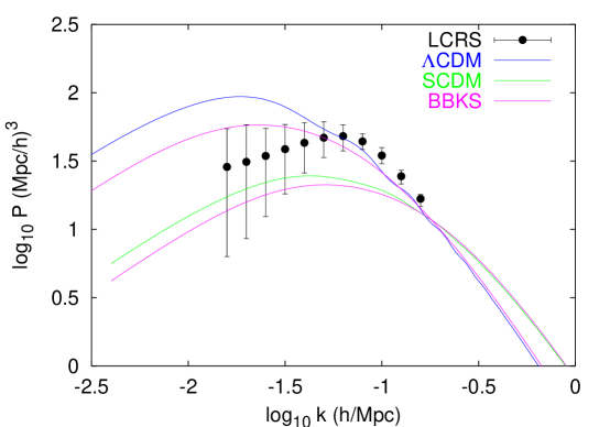
Figure 1.: Theoretical CDM power spectra compared with the deconvolved power spectrum of galaxies from the Las Campanas Redshift Survey [[19]]. The error bars are strongly correlated at large scales.

Figure 1 compares the linear power spectra extrapolated to $\tau=\tau_{0}$ (i.e. redshift 0) for several flat CDM models. The curves are all normalized so that the density smoothed with a 8 $h^{-1}$ Mpc spherical “tophat” has standard deviation $\sigma_{8}=0.9$ in agreement with observed galaxy clustering for a “linear bias factor” $b=\sigma_{8}^{-1}=1.1$. The $\Lambda$CDM model with $(\Omega_{b}=0.05,\Omega_{c}=0.30,\Omega_{\Lambda}=0.65,h=0.65)$ has the most power on large scales, possibly too much (although an acceptable fit can be found with slightly higher $\Omega_{c}$). The SCDM model with $(\Omega_{b}=0.05,\Omega_{c}=0.95,h=0.50)$ has too little power on large scales. When combined with the CMB anisotropy, this provides a strong argument for dark energy (e.g. a cosmological constant) [[20]].

The curves labeled “BBKS” show the linear power spectra for the $\Lambda$CDM and SCDM models in the limit $\Omega_{b}=0$ (with $\Omega_{c}=0.35$ and 1.0 for the two models, respectively). They are obtained from the fitting formula given by equation (G3) of [[17]] and agree well with full calculations using the COSMICS code [[21]], which was used for the other curves in Figure 1. Baryons reduce the amount of small-scale power relative to scales $k<k_{e}$ because they cannot experience gravitational instability on scales smaller than the photon-baryon Jeans length until after recombination. The oscillations in the $\Lambda$CDM power spectrum are also due to baryons and are similar to the cosine integral contributions to $\delta_{c}(k)$ in equation (51). They arise from the acoustic oscillations of the baryons between $\tau_{e}$ and $\tau_{\rm rec}$. When the power spectra are normalized at small scales (as they effectively are with $\sigma_{8}$), increasing the baryon fraction increases the amount of large-scale power.

Aside from the baryon effect, the main parameter affecting the CDM spectrum (and the only one in the BBKS formula) is $k_{e}$. As may be checked using equation (50), the peak of the CDM power spectrum is closely equal to $k_{e}$. Measurements of galaxy clustering actually constrain $k_{e}/h=0.1\Gamma$ Mpc^-1 where $\Gamma\equiv\Omega_{m}h$ is a commonly used parameter. However, as Figure 1 shows, a second parameter, the baryon fraction $\Omega_{b}/\Omega_{m}$, also significantly affects the CDM spectrum.

5.2. Evolution of Large Scale Structure

The results given above concerned the shape of the CDM power spectrum, which is frozen in after the universe becomes matter-dominated. However, the amplitude grows as $a(\tau)$ as assumed in equation (53) only if $\Omega_{m}=1$. While this is a good approximation soon after recombination, it breaks down at small redshift when $\Omega_{m}<1$ today. In this case we must include dark energy, curvature, and any other important contributor to the expansion rate of the universe.

The evolution of CDM density fluctuations for $\tau\gg\tau_{e}$ is given by equations (14) and (3.) ignoring the radiation terms. On subhorizon scales for $\phi^{2}\ll\delta_{m}^{2}\ll 1$ we have

$$\partial_{\tau}^{2}\delta_{m}+{\dot{a}\over a}\partial_{\tau}\delta_{m}=4\pi Ga^{2}\bar{\rho}_{m}\delta_{m}={3\over 2}\Omega_{m}H_{0}^{2}\,{\delta_{m}\over a}\ .$$ (57)

Because the coefficients are spatially homogeneous, the time and space dependences of the solution factor: $\delta_{m}(\vec{x},\tau)=\delta_{+}(\vec{x}\,)D_{+}(\tau)+\delta_{-}(\vec{x}\,)D_{-}(\tau)$. For $\Omega_{m}>0$, $D_{+}$ grows with time and $D_{-}$ decays. For $\Omega_{m}=1$ the growing solution is $D_{+}=a$. For $\Omega_{m}<1$ the solutions depend on the curvature $K$ (sometimes expressed as $\Omega_{K}=-K/H_{0}^{2}$) and on the equation of state of the dark energy. See Peebles [[22]] and Peacock [[15]] for examples.

Peculiar velocities offer another probe of large-scale structure that is sensitive directly to all matter, dark or luminous. The divergence of peculiar velocity $\vec{v}=d\vec{x}/d\tau$ depends on the growth rate of density fluctuations:

$$\theta_{m}\equiv\vec{\nabla}\cdot\vec{v}_{m}=-\partial_{\tau}\delta_{m}=-\left(d\ln D_{+}\over d\ln a\right)aH\delta_{m}\quad\hbox{for}\ \delta_{m}^{2}\ll 1\ .$$ (58)

Measurements of galaxy velocities actually give $\vec{v}/aH$, so that the ratio of velocity divergence to density fluctuation gives the logarithmic growth rate of density fluctuations. An empirical fit to a range of models gives $d\ln D_{+}/d\ln a=f(\Omega_{m})\approx\Omega^{0.6}$. In practice, the galaxy number density may be a biased tracer of the total matter density, conventionally parameterized by the bias factor $b$: $\delta_{\rm galaxies}=b\delta_{m}$. Comparing galaxy clustering and velocities then allows determination of $\Omega_{m}^{0.6}/b$.

5.3. Numerical Simulation Methods

Linear theory breaks down once dark matter clumps become significantly denser than the cosmic mean. Once this happens, full numerical simulations are needed to accurately follow the nonlinear dynamics of structure formation. Moreover, radiative processes, star formation, and supernova feedback have a strong effect on the baryonic component once galaxies begin forming. Although these processes can only be included in simulations in a phenomenological way, numerical simulations are still the best way to advance our theoretical understanding of structure formation deep into the nonlinear regime.

Here we present only a brief synopsis of numerical simulation methods. For a comprehensive review of both the methods and their applications see [[23]].

Particle methods are used for representing the dark matter. The phase space of dark matter is represented by a sample of particles evolving under their mutual gravitational field:

$${d\vec{x}_{i}\over d\tau}=\vec{v}_{i}\ ,\quad{d\vec{v}_{i}\over d\tau}=-{\dot{a}\over a}\vec{v}_{i}-\vec{\nabla}\phi\ ,\quad\nabla^{2}\phi=4\pi Ga^{2}\left[\sum_{j}m_{j}\delta_{\rm D}(\vec{x}-\vec{x}_{i})-\bar{\rho}_{m}(\tau)\right]$$ (59)

where $\delta_{\rm D}$ is the Dirac delta function. In practice, the particles are spread over a softening distance to avoid unphysical two-body relaxation due to large-angle scattering. (A simulation may use particles of mass $10^{9}\ M_{\odot}$, leading to unphysical tight binaries if the forces are not softened.) The art of dark matter simulation is mainly in calculating forces much faster than $O(N^{2})$ for a softening distance several orders of magnitude smaller than the simulation volume. A variety of algorithms and codes are available; see [[23]] for details.

The initial conditions for dark matter positions and velocities are given from linear theory by the Zel’dovich approximation [[7]], which relates the comoving position to its initial value $\vec{q}$, a Lagrangian variable (i.e. one that labels each particle):

$$\vec{x}(\vec{q},\tau)=\vec{q}+D_{+}(\tau)\vec{\psi}(\vec{q}\,)\ ,\quad\vec{\nabla}_{q}\cdot\vec{\psi}=-\delta_{m}\ .$$ (60)

The initial density fluctuation field $\delta_{m}(\vec{x},\tau)$ is obtained as a sample of a gaussian random field with appropriate power spectrum.

Baryon physics is added by numerical integration of the fluid equations (17) and (18) with the addition of heating and cooling, ionization, etc. There are two classes of methods in widespread use in cosmology: smoothed-particle hydrodynamics (SPH) and grid-based methods. SPH is an extension of the N-body dynamics of equations (59) to include pressure forces and thermodynamics. It has the advantage of concentrating the spatial resolution and computational effort where the baryons are densest, with the drawback of relatively large numerical viscosity and diffusivity owing to the particle discreteness. Grid-based methods use finite-difference techniques to approximate the fluid equations on a (usually) regular lattice. High accuracy methods developed for aerodynamic and other applications provide excellent resolution of shock waves, but with a resolution limited by the grid. Adaptive mesh refinement techniques are now being used to refine the resolution where needed, resulting in the ability to follow structure formation to much higher densities than previously possible [[24]].

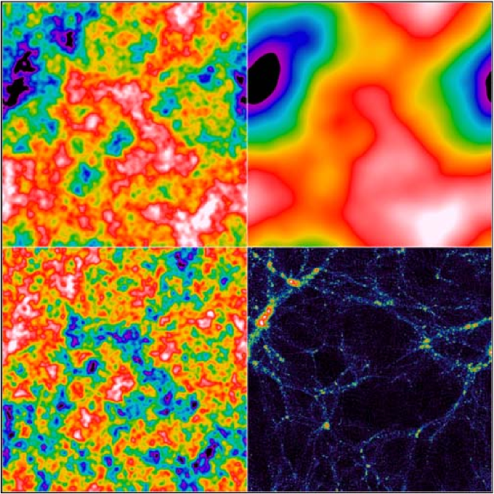
Figure 2.: Potential and density for a mixed cold+hot dark matter model with $\Omega_{\nu}=0.2$ [[25]]. A slice of size $50h^{-1}$ Mpc is shown. Upper left: potential at the end of inflation. Upper right: potential at the end of recombination. Lower left: density at the end of recombination. Lower right: density at redshift 0.

We conclude this introduction to numerical simulation methods with a mosaic of gravitational potential and dark matter density from a high-resolution simulation of the mixed cold+hot dark matter model. Figure 2 shows the linear theory and nonlinear simulation results. On the scales shown, $\Lambda$CDM would be almost indistinguishable.

The gravitational potential shown in Figure 2 is a statistical fractal at the end of inflation, viz. a gaussian random field with power spectrum $P_{A}\propto k^{-3}$. During the radiation era, acoustic damping smooths the potential on scales smaller than $k_{e}^{-1}$. Because the density fluctuations are related to the potential by two spatial derivatives, the corresponding linear density field is dominated by high spatial frequency components. Indeed, if not for the smoothing imposed by finite spatial resolution, the variance of density fluctuations would be logarithmically divergent. It is instructive to compare the post-recombination density with the inflationary potential. The density is almost proportional to the potential but with opposite sign. This is because the density/potential transfer function (52) varies only logarithmically on small scales.

The nonlinear evolution of the density field causes the mass to cluster strongly into wispy filaments and dense clumps; most of the volume has low density. The intermittency of structure is a sign of strong deviations from gaussian statistics.

5.4. Press-Schechter Theory

Numerical simulations show that most of the mass falls into dense self-gravitating clumps. As a crude approximation, let us suppose that the mass profile of every clump is spherically symmetric. In this case every gravitationally bound shell will eventually fall into the center of the clump, at a time that is dependent on the enclosed mass and energy of the shell. For linear growing mode initial conditions, collapse occurs when linear theory would predict that the mean density contrast interior to the shell is $\delta_{c}=1.686$ [[15]]. Thus, in the spherical model, the distribution of clump masses is simply dependent on the statistics of the smoothed linear density field.

Press and Schechter [[26]] devised an elegant method for computing the mass distribution of gravitationally bound clumps using the simple spherical model. Their procedure is first to smooth the linear density field by convolution with a spherical “tophat” of radius $R$ enclosing mean mass $M(R)=(4\pi/3)\bar{\rho}_{m}R^{3}$:

$$\bar{\delta}_{m}(\vec{x}\,)=\int d^{3}x^{\prime}\,W_{R}(|\vec{x}-\vec{x}^{\,\prime}|)\delta_{m}(\vec{x}^{\,\prime})\ ,\quad W_{R}(r)={3\over 4\pi R^{3}}\cases{1,\ r<R\ ,\cr 0,\ r>R\ .}$$ (61)

According to the Press-Schechter ansatz, the regions of the initial density field with $\bar{\delta}>\delta_{c}=1.686$ at time $\tau$ have collapsed into objects of mass at least $M$. It is easy to see that this would be true for a single spherical density perturbation; the genius is applying this to the entire density field.

Under this model, the fraction of mass in the universe contained in clumps more massive than $M$ is

$${1\over\bar{\rho}_{m}}\int_{M}^{\infty}dM\,M{dn\over dM}=P(\bar{\delta}>\delta_{c}|M,\tau)\ .$$ (62)

On the left-hand side, $(dn/dM)dM$ is the number density of clumps of mass in $(M,M+dM)$; the integral gives the total mass density in clumps more massive than $M$. Dividing by $\bar{\rho}$ gives the mass fraction. On the right-hand side, $P(\bar{\delta}>\delta_{c}|M,\tau)$ is the probability that a randomly chosen point in the linear density field has $\bar{\delta}>\delta_{c}$ at time $\tau$, where $M$ defines the smoothing scale of $\bar{\delta}$. For a gaussian random field of density fluctuations, this probability is simply

$$P={1\over 2}\hbox{erfc}\left(\delta_{c}\over\sigma\sqrt{2}\right)$$ (63)

where erfc is the complementary error function and $\sigma^{2}=\sigma^{2}(M,t)=\langle\bar{\delta}^{2}\rangle$ is the variance of the smoothed density. From equation (62) we can deduce $dn/dM$ by differentiating with respect to $M$.

Now, as $M\to 0$, $\sigma(M)$ grows without bound for CDM models with logarithmically diverging power on small scales, so that $P(\bar{\delta}>\delta_{c}|M=0,\tau)={1\over 2}$. Half of the mass initially is in overdense regions, half is in underdense regions $\bar{\delta}<0$ which in linear theory can never collapse. However, this is plainly unphysical, as simulations show that virtually all of the mass, including that in initially underdense regions, accretes onto dense clumps. Thus, Press and Schechter suggested doubling $dn/dM$ so that all of the mass resides in dense clumps. Thus, their formula for the mass distribution of clumps is

$${dn\over dM}={2\bar{\rho}\over M}{\partial P\over\partial M}\ .$$ (64)

Although realistic gravitational collapse is far more complex than imagined in this derivation, equation (64) gives surprisingly good agreement with clump masses measured in cosmological N-body simulations [[27]]. The Press-Schechter model and its generalizations have proved to be a very useful tool for comparing ab initio theories (power spectrum and cosmological model) with observations of galaxies and galaxy clusters.

6. Conclusions

These lecture notes have presented a few of the theoretical elements useful for understanding the microwave background and structure formation. Cosmology is rapidly changing with the advent of precision measurements of CMB anisotropy, with the observation of galaxies at $z>3$, and with large new redshift surveys. Theoretical research has become more phenomenological, with a focus on providing the framework for interpreting and analyzing the new data. Despite this trend—or perhaps because of the high quality of new data—theoretical cosmology still requires further development of the basic processes of structure formation. Either way, I hope that the material presented in these lectures will be useful to cosmology graduate students.

Acknowledgments.

I would like to thank Sergei Bashinsky for help with the two-fluid solutions. I am grateful to the organizers, the other speakers, and the students of the Cosmology 2000 summer school for the fruitful, stimulating atmosphere in Lisbon. Special thanks are due to the organizers for their wonderful hospitality. This work was supported by NSF grant AST-9803137.

References

- 1 [1] E. Bertschinger, in Cosmology and Large Scale Structure, proc. Les Houches Summer School, Session LX, ed. R. Schaeffer, J. Silk, M. Spiro, and J. Zinn-Justin, Elsevier Science, Amsterdam (1996) 273.
- 2 [2] C.-P. Ma and E. Bertschinger, ApJ 455 (1995) 7.
- 3 [3] E. M. Lifshitz, J. Phys. USSR 10 (1946) 116.
- 4 [4] C.W. Misner, K.S. Thorne, and J.A. Wheeler, Gravitation, Freeman, San Francisco (1973).
- 5 [5] Gravity Probe B website, http://einstein.stanford.edu/.
- 6 [6] J.M. Bardeen, Phys.Rev.D 22 (1980) 1882.
- 7 [7] Ya.B. Zel’dovich, A&A 5 (1970) 84.
- 8 [8] P.J.E. Peebles and R.H. Dicke, ApJ 154 (1968) 891.
- 9 [9] U. Seljak and M. Zaldarriaga, ApJ 469 (1996) 437.
- 10 [10] W. Hu, U. Seljak, M. White, and M. Zaldarriaga, Phys.Rev.D 57 (1998) 3290.
- 11 [11] P. Schneider, J. Ehlers, and E.E. Falco, Gravitational Lenses, Springer-Verlag, Berlin (1992).
- 12 [12] U. Seljak, ApJ 463 (1996) 1.
- 13 [13] P.J.E. Peebles and J.T. Yu, ApJ 162 (1970) 815.
- 14 [14] R.K. Sachs and A.M. Wolfe, ApJ 147 (1967) 73.
- 15 [15] J.A. Peacock, Cosmological Physics, Cambridge Univ. Press (1999).
- 16 [16] S. Bashinsky and E. Bertschinger, astro-ph/0012153.
- 17 [17] J.M. Bardeen, J.R. Bond, N. Kaiser, and A.S. Szalay, ApJ 304 (1986) 15.
- 18 [18] E.R. Harrison, Phys.Rev.D 1 (1970) 2726.
- 19 [19] H. Lin et al., ApJ 471 (1996) 617.
- 20 [20] M. Tegmark, M. Zaldarriaga, and A.J.S. Hamilton, astro-ph/0008167.
- 21 [21] E. Bertschinger, astro-ph/9506070 and http://arcturus.mit.edu/cosmics/.
- 22 [22] P.J.E. Peebles, The Large-Scale Structure of the Universe, Princeton Univ. Press (1980).
- 23 [23] E. Bertschinger, ARA&A 36 (1998) 599.
- 24 [24] T. Abel, G.L. Bryan, and M.L. Norman, ApJ 540 (2000) 39.
- 25 [25] C.-P. Ma and E. Bertschinger, ApJ 434 (1994) L5.
- 26 [26] W.H. Press and P. Schechter, ApJ 187 (1974) 425.
- 27 [27] S. Cole and C. Lacey, MNRAS 281 (1996) 716.