*

Abstract

In this talk I propose the first fast methods which can analyze CMB data taking into account correlated noise, arbitrary beam shapes, non-uniform distribution of integration time on the sky, and partial sky coverage, without the need for approximations. These ring torus methods work by performing the analysis in the time ordered domain (TOD) rather than on the sky map of fluctuations. They take advantage of the simplicity of noise correlations in the TOD as well as certain properties of the group of rotations SO(3). These properties single out a family of scanning strategies as favorable, namely those which scan on rings and have the geometry of an n-torus. This family includes the strategies due to TOPHAT, MAP and Planck. I first develop the tools to model the time ordered signal, using Fast Fourier Transform methods for convolution of two arbitrary functions on the sphere (Wandelt and Górski 2000)[1]. Then I apply these ideas to show that in the case of a 2-torus one can reduce the time taken for CMB power spectrum analysis from an unfeasible order $N^{3}$ to order $N^{2}$, where $N\sim 10^{5}-10^{8}$ is the number of resolution elements (Wandelt and Hansen, in preparation)[2].

1 Introduction

A major near-term objective in the field of Cosmology today is to gain a detailed measurement and statistical understanding of the anisotropies of the cosmic microwave background (CMB). While the theory of primary CMB anisotropy is well-developed (see [3] for a review) and we are facing a veritable flood of data from a new generation of instruments and missions, the single most limiting hurdle are the immense computational challenges one has to overcome to analyze these data[4, 5, 6].

Let me outline the key problems involved. The goal is to derive two things: an optimal sky map estimate and a set of power spectrum estimates $\widehat{C}_{l}$ which, for a Gaussian CMB sky are a sufficient statistic, highly informative about cosmological parameters. In this talk I will focus on the $\widehat{C}_{l}$ estimation problem, but the ideas I develop can be usefully employed for map-making as well.

The analysis problem involves maximizing the likelihood given the data as a function of these $\widehat{C}_{l}$. If the observed CMB anisotropy is written as a vector $d$ the likelihood takes the form

$${\cal L}(C_{l}|d)=\frac{\exp\left[{-\frac{1}{2}{\bf d}^{T}({\bf S}(C_{l})+{\bf N})^{-1}{\bf d}}\right]}{\sqrt{(2\pi)^{N_{d}}|({\bf S}(C_{l})+{\bf N})|}},$$ (1)

where the signal covariance matrix $\bf{S}$ is a function of the $C_{l}$, ${\bf N}$ is the noise covariance matrix and $N_{d}$ is the number of entries in the data vector $d$. If ${\bf S+N}$ is a general matrix, evaluating the inverse and determinant in this quantity takes ${{\cal O}\!\left(N^{3}_{d}\right)}$ operations.

Commonly the data vector is taken to be a set of sky map pixels, with $N_{d}\sim 10^{5}-10^{8}$. Hence entries in $\bf{S}$ and ${\bf N}$ are the covariances between two positions on the celestial sphere. Alternatively one can choose the spherical harmonic basis. Other bases have also been suggested, such as cut sky harmonics [7] and signal to noise eigenmodes [8], but changing into these more general bases takes ${{\cal O}\!\left(N_{d}^{3}\right)}$ operation.

Borrill (in these proceedings) presented a careful review of the computational tasks involved in solving this maximization problem in the general case, using state-of-the-art numerical methods. The conclusion is that in their present form these methods fail to be practical for forthcoming CMB data sets. Given the major international effort currently under way to observe the CMB (see, e.g. [9, 10, 11]), finding a solution to this problem is of paramount importance.

The underlying reason for this failure is that the signal covariance matrix ${\bf S}$ and noise covariance matrix ${\bf N}$ are usually very differently structured. In pixel space, ${\bf S}$ is full, while ${\bf N}$ is ideally sparse (for a well-controlled experiment). In spherical harmonic space we are in the opposite regime. For all-sky observations, ${\bf S}$ would be diagonal while the form of ${\bf N}$ depends on experimental details and observational strategy of the mission and in general could be any covariance matrix at all. Therefore the quantity which enters in the likelihood ${\bf C\equiv S+N}$ is not sparse in any easily accessible basis.

In this talk I exhibit a solution to this dilemma. In the following section I will point out that modeling realistic observations in the time ordered domain simplifies the problem. In particular, one can take advantage of the simple covariance structure of the noise in the time ordered data (TOD). To be able to formulate the likelihood problem in terms of the TOD one needs to be able to compute the expected signal correlations in the TOD. I achieve this using the Wandelt-Górski method for fast convolution on the sphere [1] which I briefly review in section 3. In section 4 I show that this implies that the signal correlations have a special structure for certain types of scanning strategies namely those where the TOD can be thought of as being wrapped on an n-torus. This happens to be true for the planned scanning strategies for TOPHAT and Planck (n=2), as well as MAP (n=3).

Using the results from these geometrical ideas I go on to formulate the likelihood problem for the $C_{l}$ on this ring torus, with both ${\bf S}$ and ${\bf N}$ sparse. In fact, they are both block-diagonal with the same pattern of blocks; hence ${\bf C}$ is also block diagonal.

This is the first example of a fast maximum likelihood estimator which can analyze CMB data in the presence of correlated noise. We will see below that it can also deal with non-uniform distribution of integration time, beam distortions, far side lobes, and partial sky coverage, all without needing to invoke approximations.

The exact computational scaling of the evaluation of ${\cal L}$ depends somewhat on the scanning strategy used, but if the ring torus is an 2-torus it takes only ${{\cal O}\!\left(N^{2}\right)}$ operations. For TOPHAT and one of the proposed Planck scanning strategies, the ring torus is a 2-torus, for a precessing scan such as MAP’s it is a 3-torus. For simplicity I only deal with the 2-torus case here. Generalizations to $n\geq 3$ are trivial and they will be discussed in [2]. This forthcoming paper will also contain a presentation of the results of applying this method to simulated data.

2 The Case for Analyzing CMB Data in the Time-Ordered Domain

Why is power spectrum analysis of estimated sky maps so difficult?

1) Correlated noise.

The CMB anisotropies are very small. This means that measurements are noisy. Current detectors have the feature that they add correlated noise to the signal. If we can assume that the correlated noise is stationary and circulant then it has a very simple correlation structure in Fourier space. But estimating the sky from the TOD projects these simple correlations into very complicated noise correlations between separated pixels, which are visible as striping in the maps.

2) Non-uniform distribution of integration time.

For most missions, practical constraints on the scanning strategy force the available integration time to be allotted non-uniformly over the sky. This leads to coupling of the noise in spherical harmonic space, in addition to coupling due to partial sky coverage (see item 4 below). However, in the TOD, integration time per sample is constant, by definition.

3) Beam distortions and far side lobes.

Microwaves are macroscopic, with wavelengths of order a few $mm$ to a few $cm$. Hence they will diffract around macroscopic objects. This leads to distorted point spread functions and far side lobes. Simulations have to convolve these asymmetric beams with an input sky with foreground signals varying over many orders of magnitude from place to place. Analyses have to deconvolve the observations to make accurate inferences about the underlying sky.

4) Partial sky coverage.

The cosmological information is most visible in spherical harmonic space. In a homogeneous and isotropic Universe, where the perturbations are Gaussian, the power spectrum $C_{l}$ completely encodes the statistical information which is present in a map of fluctuations. Statistical isotropy of the fluctuations around us also implies that the spherical harmonics $Y_{lm}$ are the natural basis for representing the CMB sky. But due to local foregrounds that need to be excised from the map or partial sky coverage this isotropy is broken in actual data sets. This introduces additional signal and noise correlations in $Y_{lm}$ space, because there is a geometrical coupling between $Y_{lm}$ of different $l$ and $m$.

There are currently no exact and fast methods that can deal with all of these issues.

In order to avoid issue 1), MAP has been designed to have very small correlations between the noise in separated pixels. A numerically exact $N^{2}$ maximum likelihood method [12] and a nearly optimal, unbiased $N^{3/2}$ method [13] have been proposed which can deal with issues 2) and 4) but not 3). So even without correlated noise the results of this paper may be interesting for building future MAP power spectrum analysis methods, should the issues of beam distortions and far side lobes be important.

But both TOPHAT and Planck will produce striped data sets beyond the capability of these or any current algorithms. Hence, being able to deal with noise correlations is paramount to the success of these missions.

It is clear from 1) and 2) that the noise properties are much simpler in the TOD than in a sky map. But what about the signal correlations? What is the price of forfeiting the advantages of the sphere for representing statistically isotropic signals? In the next section I will demonstrate that one can devise scanning strategies which break only part of the symmetries of the sphere and make the signal correlations in the TOD as simple as the noise properties.

3 Modeling the Signal in the Time-Ordered Domain Using the Fast Convolution Algorithm

Recently, Wandelt and Górski (2000) [1] have introduced new methods for greatly speeding up convolutions of arbitrary functions on the sphere. This reference contains a detailed description of methods which will enable future missions such as MAP and Planck to take beam imperfections into account without resorting to approximations. The algorithm is completely general and can be applied to any kind of directional data, even tensor fields [14]. I will now briefly review the ideas and quote the results.

Figure 1: A geometrical representation of the output of our most general convolution method. The fact that we are dealing with arbitrary functions means that the results are a function of the orientation of the beam with respect to the sky not just the direction it is pointing in. Therefore we need three Euler angles to parameterize the results as shown, as rings attached to each point on the sphere. Note that this representation is a double cover of SO(3) because a right handed rotation about a given direction is equivalent to a left handed rotation about the opposite direction

What do I mean by convolution on the sphere? Mathematically, the convolution lives in the group of rotations SO(3), because one has to keep track of the full relative orientation of the beam to the sky, not just the direction it points in. To specify the relative orientation one can use the Euler angles $\Phi_{1},\Theta$ and $\Phi_{2}$. The convolved signal for each beam orientation $(\Phi_{1},\Theta,\Phi_{2})$ can then be written as

$$T^{S}(\Phi_{2},\Theta,\Phi_{1})=\int d\Omega_{\vec{\gamma}}\,\left[\widehat{D}(\Phi_{2},\Theta,\Phi_{1})b\right]\!\!(\vec{\gamma})^{\ast}s(\vec{\gamma}).$$ (2)

Here the integration is over all solid angles, $\widehat{D}$ is the operator of finite rotations such that $\widehat{D}b$ is the rotated beam, and the asterisk denotes complex conjugation. Figure 1 gives a geometrical representation of the result of such a convolution. The fact that the beam is not assumed to be azimuthally symmetric means that at each point on the sphere, there is a ring of different convolution results corresponding to all relative orientations about this direction.

If ${\sf{L}}$ measures the inverse of the smallest length scale in the smoother of the sky or beam, the numerical evaluation of the integral in Eq. (2) takes ${{\cal O}\!\left({\sf{L}}^{2}\right)}$ operations for each tuple $(\Phi_{1},\Theta,\Phi_{2})$. To allow subsequent interpolation at arbitrary locations it is sufficient to discretize each Euler angle into ${{\cal O}\!\left({\sf{L}}\right)}$ points and thus we have ${{\cal O}\!\left({\sf{L}}^{3}\right)}$ combinations of them. As a result, the total computational cost for evaluating the convolution using Eq. (2) scales as ${{\cal O}\!\left({\sf{L}}^{{5}}\right)}$ .

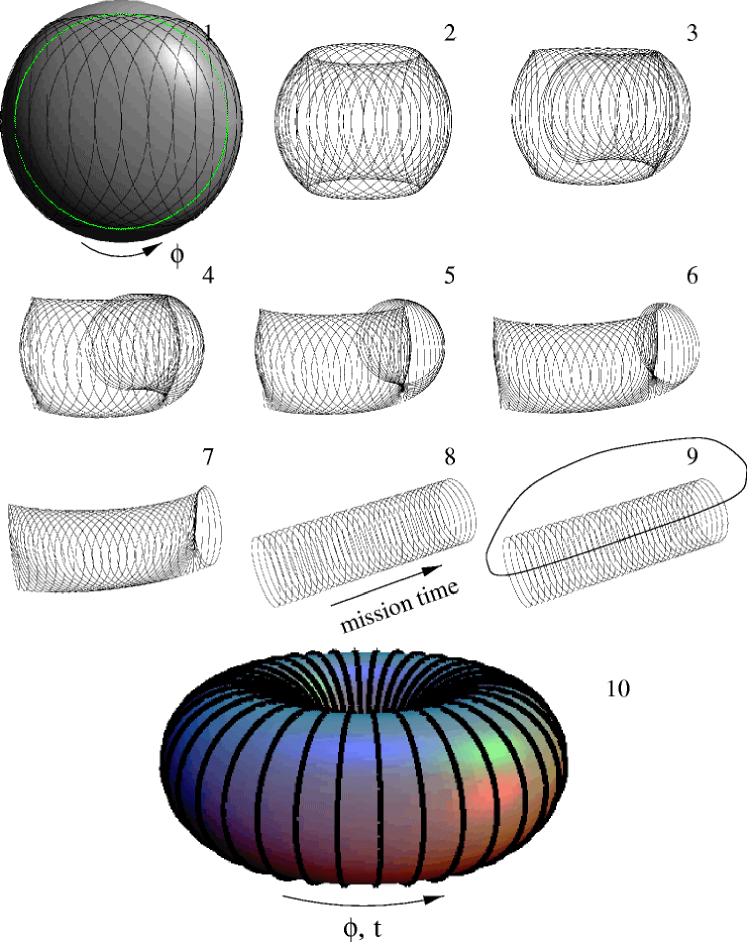
Figure 2: The correspondence between a basic scan strategy (1 and 2), the ring set (8) and a 2 dimensional ring torus (10)

It turns out that by Fourier transforming the above equation on the Euler angles (after applying a judiciously chosen factorization) we can reduce this scaling to ${{\cal O}\!\left({\sf{L}}^{{4}}\right)}$ in general. One can further reduce the scaling to ${{\cal O}\!\left({\sf{L}}^{3}\right)}$ if one is only interested in the convolution over a path which consists of a ring of rings at equal latitude around the sphere. We called such configurations basic scan paths in reference [1]. One example, covering a large part of the sphere, is shown in Figures 2.1 and 2.2.

Figure 2 illustrates that a basic scan path is geometrically a 2-torus and Figure 3 shows how to cut and unfold the torus for easy visualization.

I quote here the formula for the Fourier coefficients of the convolved signal on this ring torus [1]. If the convolved signal on the ring torus is $T^{S}_{rp}$ with $r$ counting the ring number and $p$ the pixel number on the ring, then its Fourier coefficients are

$$T^{S}_{m\,m^{\prime}}(\omega=0)=\sum_{l}s_{lm}d^{l}_{mm^{\prime}}(\theta_{E})X_{lm^{\prime}}.$$ (3)

Here the $s_{lm}$ are the spherical harmonic multipoles for the CMB sky and $\theta_{E}$ fixes the latitude of the spin axis on the sky. The quantity

$$X_{lm}\equiv\sum_{M}d^{l}_{mM}(\theta)b_{lM}^{\ast}$$ (4)

is just the rotation of the beam multipoles $b_{lm}$ for an arbitrary beam by $\theta$, the opening angle of the scan circle. $X_{lm}$ can be precomputed. Counting indices in Eq. (3) confirms that computing the convolution along a basic scan path takes only $\sim{\sf{L}}^{3}$ operations.

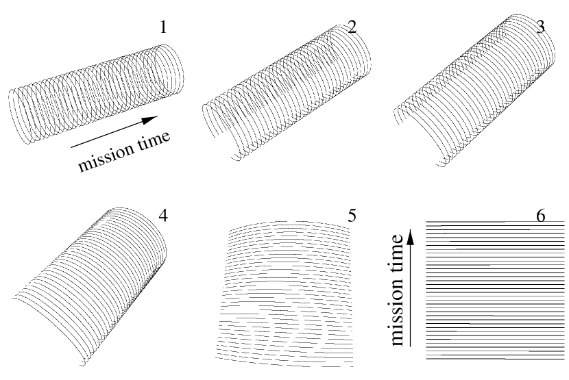
Figure 3: Here I show continuing from Figure 2.8 how to present the convolved signal in the ring set (1) as a two dimensional density plot where the rings are cut, extended into lines, and stacked vertically (6)

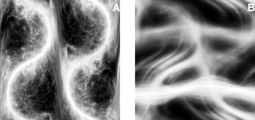
Figure 4: Here I show the ring set that results from the fast convolution algorithm along a basic scan path in the representation shown in Figure 3.6. In both (A) and (B) I used the Schlegel Finkbeiner Davis model of dust emission [15] at 100GHz, sampled on $\sim 10^{7}$ pixels and the worst Plank LFI horn with a main beam size of about 30 arcminutes FWHM. Part (A) shows the convolution using only the 5 degrees of the beam around the main beam and part (B) shows the convolution with the full far side lobe pattern, excluding the inner 5 degrees. The beam and sky vary over many orders of magnitude. In (B) even discreteness effects of the ECP pixels which represented the beam side lobes can be seen

Figure 4 shows the results of such a convolution for the main beam (inner 5 degrees) and the far side lobes (everything except the inner 5 degrees) of the physical model of one Planck LFI 30GHz horn. The nominal resolution of this horn is 30 arcminutes FWHM. This computation of $4\times 10^{6}$ convolved samples from the Schlegel Finkbeiner Davis dust emission model [15] at 100 GHz ($12\times 10^{6}$ pixels) took $\sim 15$ minutes. That compares with a projected time of several months if the integrals had been done in pixel space, even when using efficient grids of varying resolution.

4 Ring Torus Analysis: Beating the Big $N^{3}$

Using the results from the previous section we can now write down an statistical model of the time-ordered data as a function of the $C_{l}$ and experimental parameters.

I will first derive the signal-correlation matrix as a function of the $C_{l}$ and then go on to derive the noise correlation as a function of instrumental parameters (like the shape of the noise power spectrum in the TOD) and the scanning strategy (in this case the dimensions and position of the basic scan path). Detailed derivations can be found in [2].

4.1 Signal Correlations

What we are interested in are the correlation properties of the signal on the ring torus, Eq. (3). We can now easily compute the correlation matrix

$${\cal T}^{S}_{m\,m^{\prime}\;M\,M^{\prime}} \equiv \left\langle T^{S}_{m\,m^{\prime}}T^{S}_{M\,M^{\prime}}\right\rangle$$ (5)

$$= \framebox{$\delta_{mM}$}\sum_{l}C_{l}d^{l}_{mm^{\prime}}(\theta_{E})X_{lm^{\prime}}d^{l}_{MM^{\prime}}(\theta_{E})X_{lM^{\prime}}.$$ (6)

The boxed Kronecker delta shows that the correlation matrix in Fourier space on the ring torus is block diagonal.

4.2 Noise Correlations

I start by assuming that we can model the noise in the time ordered domain as a stationary Gaussian process whose Fourier components $\widetilde{T}^{N}_{k}$ have the property

$$\left\langle\widetilde{T}^{N}_{k}\widetilde{T}^{N\ast}_{k^{\prime}}\right\rangle=P(k)\delta_{kk^{\prime}}.$$ (7)

The noise power spectrum in the time-ordered domain is well described for practical purposes as $P(k)=\sigma^{2}[1+(k_{knee}/k)^{\alpha}]$, with $\alpha\in]0,2]$.

In the following I will allow for the complication that the scanning strategy involves integrating repeatedly on a fixed ring then the signal remains the same for each scan of that ring. One can just co-add all scans over the same ring without losing information.

To be specific, if we define $N_{R}$ to be the number of pixels per ring, $N_{s}$ the number of times the satellite spins while observing a fixed ring, and $N_{r}$ to be the number of rings for a one-year mission, we can write $N_{TOD}=N_{R}N_{s}N_{r}$ for the number of samples in the TOD. In the following I will choose $N_{r}=N_{R}$ for simplicity, though this is not required by the formalism and can be generalized trivially. The ring torus will then have $N_{r}^{2}$ elements.

These properties of the noise covariance in the time-ordered data allow writing the noise covariance on the ring set as [2]

$$\left\langle{T}^{N}_{rp}{T}^{N\ast}_{r^{\prime}p^{\prime}}\right\rangle\equiv C(r-r^{\prime},p-p^{\prime}),$$ (8)

where $C$ is periodic with period $N_{r}$ in its first entry; letting $\Delta\equiv r-r^{\prime}$ we have

$$C(\Delta,p-p^{\prime})=C(\Delta+jN_{r},p-p^{\prime}),\quad j\in{\cal Z}.$$ (9)

This implies for the covariance of the Fourier components of the the co-added noise on the rings

$${\cal T}^{N}_{m^{\prime}mM^{\prime}M} \equiv \left\langle\widetilde{T}^{N}_{m^{\prime}m}\widetilde{T}^{N\ast}_{M^{\prime}M}\right\rangle$$ (10)

$$= \frac{1}{(N_{r})^{3}}\framebox{$\delta_{mM}$}\sum_{p,p^{\prime}=0}^{N_{r}-1}e^{-\frac{2\pi i}{N_{r}}(m^{\prime}p-M^{\prime}p^{\prime})}\sum_{\Delta=0}^{N_{r}-1}e^{-\frac{2\pi i}{N_{r}}m\Delta}C(\Delta,p-p^{\prime})$$ (11)

where I used (9) to obtain the boxed Kronecker delta which flags that the noise covariance is block diagonal on the ring torus in exactly the same way as the signal.

4.3 From $N^{3}$ to $N^{2}$: Why it Works and Other Advantages

I just showed that by choosing the scanning strategy such that the TOD can be wrapped (co-added) onto a 2-torus one can find a basis in which both noise and signal are block diagonal and hence sparse. What is more, the data can be easily transformed into this basis just by computing the Fast Fourier Transform of the co-added TOD.

Why does it work? The ring torus exhibits a spatio-temporal symmetry: time proceeds linearly around the torus, (“$t$” in Figure 2.10), in the same direction as the azimuthal angle (“$\phi$” in Figure 2.1 and 2.10). Stationarity of the noise in the TOD and isotropy of the signal on the sphere are of course broken on the torus, but both show up as a “partial isotropy” (only in the azimuthal direction), which expresses itself as a simplified correlation structure in Fourier space.

One can therefore write down the likelihood Eq. (1) on the ring torus by simply substituting

$$d_{\rm map}\rightarrow d_{\rm ring~{}torus},\quad{\bf S}\rightarrow{\cal T}^{S},\quad{\bf N}\rightarrow{\cal T}^{N}$$ (12)

Due to the block diagonality, the inverse and determinant in the Eq. (1) only take ${{\cal O}\!\left(N^{2}\right)}$ operations to evaluate. The gradient is similarly easy to evaluate

$$-2\frac{\partial\ln{\cal L}}{\partial C_{l}}=Tr({\bf C}^{-1}{\bf C,}_{C_{l}})-d^{T}{\bf C}^{-1}{\bf C,}_{C_{l}}{\bf C}^{-1}d$$ (13)

which only takes ${{\cal O}\!\left({\sf{L}}^{3}\sim N^{3/2}\right)}$ operations to compute for each component.

Other than speed there are other advantages of ring torus methods. First, this approach bypasses map-making on the sphere for the purposes of power spectrum estimation. Not having to make maps first, helps avoiding questions like “What does my favorite de-striping algorithm do to the signal?”. On the ring torus, one fully models the striping due to correlated noise and hence does not rely on such ad hoc methods.

While the sky map is not necessarily the best starting point for the purposes of $C_{l}$ estimation, one should of course make the best map one possibly can in order to identify systematic errors etc.. Reference [1] shows how the ring torus speeds up iterative methods for deconvolving with asymmetric beams. The block diagonal noise correlations on the torus mean that one can use the same geometrical ideas for solving the map making equations in the presence of noise.

In fact both signal and noise covariances are sparse in this basis, hence this method can be used to quickly Wiener filter the data on the ring torus once the $C_{l}$ are known to optimally estimate the map of CMB fluctuations.

5 Possible Extensions and Conclusions

In this talk I constructed for the first time an exact formulation of the maximum likelihood problem of power spectrum analysis on the sphere which can deal with correlated noise, realistic beams, partial sky coverage, and non-uniform noise with a computational scaling of ${{\cal O}\!\left(N^{2}\right)}$ . This is a significant advance over other available exact methods with the same scaling, all of which assume white noise and azimuthally symmetric beams amongst other assumptions.

But however more realistic this approach is, real observations will still be more complicated. In the case of nearly all sky observations, I have not showed how to deal with small areas where foregrounds dominate such as dust emission from the galactic plane, or bright point sources. Also, irregularities in the scanning strategy will somewhat spoil the symmetry of spatial correlations in the signal and temporal correlations in the noise which the ring torus exploits.

While it is hopeless to attempt to address these further complications using current methods, I hope that ring torus methods provide a new avenue of investigation. The idea is that perturbation theory is powerful but only works when exact solutions are known. So I propose to use exact inverses, computed using the methods I presented in this talk as preconditioners to speed up conjugate gradient methods for computing $C^{-1}d$ for more general cases, e.g. galactic cuts, point sources and imperfect scanning. This is analogous to the approach of the authors of [12] who built numerical tools for the MAP analysis by perturbing around an exact solution for azimuthal sky cuts.

Under the stated assumptions I have shown that the power spectrum analysis problem simplifies greatly when it is considered in the domain of co-added time-ordered data which has the geometry of a torus. Extensions of the formulae I presented here to more general scanning strategies (e.g. a precessing scan, such as MAP’s or another proposal for Planck) are easy to derive using the more general results of [1]. In this case the efficiency depends on the size of the extra dimensions which the torus acquires.

If beam distortions and far side lobes are an issue, but noise correlations are not, then it may be more efficient to perform the analysis on a 3 torus which does not follow the scanning strategy, but parameterizes the full group of rotations SO(3) of the beam with respect to the sky and uses the total convolution formula mentioned in [1]. This still allows using FFTs, but takes advantage of the fact that azimuthal beam asymmetries are usually mild. This returns an ${{\cal O}\!\left(N^{2}\right)}$ method with a prefactor depending on the number of harmonics needed to model the azimuthal beam asymmetry. Note that in this case the scanning strategy is not constrained — but it should preferably visit every point on the sky and cover it with many different beam orientations so the group manifold of SO(3) is covered densely.

Once it is possible to deal with correlated noise, the fear of striping that has haunted the field is mitigated. Imagine that given a fixed rms noise amplitude we could choose how much of it we would like to be white and how much we would like to be correlated. What should we wish for? Actually, we should wish for maximally correlated noise! Correlated noise has regularity in it, which can be modeled, and hence removed as long as it does not mimic the signal we want to measure. White noise can never be removed, only at the expense of smoothing out structure in the signal.

I am grateful to the conference organizers for an excellent meeting, A. J. Banday, K. Górski, F. Hansen for valuable discussions and enjoyable collaborations and to the NASA MAP/MIDEX program for support.

References

- [1] B. D. Wandelt and K. M. Górski, Phys. Rev. D, in press (2001).
- [2] B. D. Wandelt and F. K. Hansen, CMB data analysis using the time ordered data , in preparation (2001).
- [3] W. Hu, N. Sugiyama, and J. Silk, Nature 386, 37 (1997).
- [4] J. Borrill, Phys. Rev. D59, 027302 (1999).
- [5] K. M. Gorski, E. F. Hivon and B. D. Wandelt,Analysis Issues for Large CMB Data Sets, astro-ph/9812350, in “Evolution of Large Scale Structure”, A. J. Banday et al. (Eds) (1998).
- [6] J. R. Bond, R. G. Crittenden, A. H. Jaffe, and L. Knox, Computing in Science and Engineering 1, (1999).
- [7] K. M. Gorski, Astrophys. J. Lett., 430, L85 (1994).
- [8] M. Tegmark, A. Taylor, and A. Heavens, Astrophys. J. 480, 22 (1997).
- [9] Tophat WWW-site, http://topweb.gsfc.nasa.gov/
- [10] Bennett, C. L. et al.1996, Microwave Anisotropy Probe: A MIDEX Mission Proposal, see also http://map.gsfc.nasa.gov/
- [11] Bersanelli et al.1996, COBRAS/SAMBA: Report on the Phase A Study, see also http://astro.estex.esa.nl/Planck/.
- [12] S. P. Oh, D. N. Spergel, and G. Hinshaw, Astrophys. J. 510, 551 (1999).
- [13] B. D. Wandelt, E. F. Hivon, K. M. Gorski, astro-ph/9808292; B. D. Wandelt, K. M. Gorski, E. F. Hivon, astro-ph/0008111, submitted to Phys. Rev. D.
- [14] A. Challinor et al., astro-ph/0008228, Phys. Rev. D,
- [15] D. Schlegel, D. Finkbeiner, and M. Davis, Astrophys. J. 500, 525 (1998).