Towards a Precise Measurement of Matter Clustering: Lyman-alpha Forest Data at Redshifts 2-4

Abstract

We measure the filling factor, correlation function, and power spectrum of transmitted flux in a large sample of Ly$\alpha$ forest spectra, comprised of 30 Keck HIRES spectra and 23 Keck LRIS spectra. We infer the linear matter power spectrum $P(k)$ from the flux power spectrum $P_{F}(k)$, using an improved version of the method of Croft et al. (1998) that accounts for the influence of redshift-space distortions, non-linearity, and thermal broadening on the shape of $P_{F}(k)$. The evolution of the shape and amplitude of $P(k)$ over the redshift range of the sample ($z\approx 2-4$) is consistent with the predictions of gravitational instability, implying that non-gravitational fluctuations do not make a large contribution to structure in the Ly$\alpha$ forest. Our fiducial measurement of $P(k)$ comes from a subset of the data with $2.3<z<2.9$, mean absorption redshift $\langle z\rangle=2.72$, and total path length $\Delta z\approx 25$. It has a dimensionless amplitude $\Delta^{2}(k_{p})=0.74^{+0.20}_{-0.16}$ at wavenumber $k_{p}=0.03({\rm km\;s}^{-1})^{-1}$ and is well described by a power-law of index $\nu=-2.43\pm 0.06$ or by a CDM-like power spectrum with shape parameter ${\Gamma^{\prime}}=1.3^{+0.7}_{-0.5}\times 10^{-3}({\rm km\;s}^{-1})^{-1}$ at $z=2.72$ (all error bars $1\sigma$). The correspondence to present day $P(k)$ parameters depends on the adopted cosmology. For $\Omega_{m}=0.4$, $\Omega_{\Lambda}=0.6$, the best-fit shape parameter is $\Gamma=0.16h\,{\rm Mpc}^{-1}$, in good agreement with measurements from the 2dF Galaxy Redshift Survey, and the best-fit normalization is $\sigma_{8}=0.82(\Gamma/0.15)^{-0.44}$. Matching the observed cluster mass function and our measured $\Delta^{2}(k_{p})$ in spatially flat cosmological models requires $\Omega_{m}=0.38^{+0.10}_{-0.08}+2.2(\Gamma-0.15)$. Matching $\Delta^{2}(k_{p})$ in COBE-normalized, flat CDM models with no tensor fluctuations requires $\Omega_{m}=(0.29\pm 0.04)n^{-2.89}h_{65}^{-1.9}$, and models that satisfy this constraint are also consistent with our measured logarithmic slope. The Ly$\alpha$ forest complements other observational probes of the linear matter power spectrum by constraining a regime of redshift and lengthscale not accessible by other means, and the consistency of these inferred parameters with independent estimates provides further support for a cosmological model based on inflation, cold dark matter, and vacuum energy.

1. Introduction

Over the last few years, the study of the Ly$\alpha$ forest has been revolutionized by high-resolution spectra (mostly using the HIRES spectrograph [Vogt et al.  1994] on the Keck telescope), by measurements of coherent absorption along lines of sight to quasar pairs (Bechtold et al. 1994; Dinshaw et al. 1994; Crotts & Fang 1998), and by a new theoretical understanding made possible by cosmological hydrodynamic simulations (e.g., Cen et al. 1994; Zhang, Anninos, & Norman 1995; Petitjean, Mücket, & Kates 1995; Hernquist et al. 1996; Wadsley & Bond 1996; Theuns et al. 1998). In these simulations the physical state of the diffuse intergalactic gas responsible for the Ly$\alpha$ forest is relatively simple, implying a direct connection between Ly$\alpha$ absorption and the underlying density and velocity fields similar to that in some analytic models of the forest (e.g., McGill 1990; Bi 1993; Bi & Davidsen 1997; Hui, Gnedin, & Zhang 1997). Several methods have been proposed for using the forest to measure the amplitude of mass fluctuations (Gnedin 1998; Gaztañaga & Croft 1999; Nusser & Haehnelt 1999), the matter power spectrum (Croft et al. 1998, hereafter CWKH; Hui 1999; McDonald & Miralda-Escudé 1999; Feng & Fang 2000; Hui et al. 2000), and the geometry of the universe (Hui 1999; McDonald & Miralda-Escudé 1999). Observational Ly$\alpha$ forest data have been used to constrain these quantities by Croft et al. (1999b, hereafter CWPHK), McDonald et al. (2000, hereafter M00), and Nusser & Haehnelt (2000). In this paper we present flux statistics measured from two large samples of Keck Ly$\alpha$ forest spectra, and we use them to measure the linear matter power spectrum with an improved version of the method presented in CWKH. The data sample represents a fourfold increase in total length of spectra compared to that in CWPHK, and it includes high resolution spectra that enable us to extend our measurement to smaller scales. The higher statistical precision of this data set requires that we address systematic errors that were not significant in our earlier measurement, and much of this paper is devoted to assessing and correcting for these systematic effects.

Our analysis breaks into two parts: a measurement of the power spectrum of transmitted flux in the Ly$\alpha$ forest, and an inference of the matter power spectrum from the flux power spectrum. The theoretical model that motivates our method for the second step is the “Fluctuating Gunn-Peterson Approximation” (FGPA; see Rauch et al. 1997; CWKH; Weinberg et al. 1998b), which describes the relation between Ly$\alpha$ opacity and matter density for the diffuse intergalactic gas that produces most of the Ly$\alpha$ forest absorption at high redshift. Photoionization heating by the ultraviolet (UV) background radiation and adiabatic cooling by the expansion of the universe combine to drive most of the gas with $\rho_{b}<10$ onto a power-law temperature-density relation,

$$T=T_{0}\rho_{b}^{\alpha},$$ (1)

where $\rho_{b}$ is the baryon overdensity in units of the cosmic mean (Katz, Weinberg & Hernquist 1996; Hui & Gnedin 1997). The parameters $T_{0}$ and $\alpha$ depend on the reionization history and on the spectral shape of the UV background; they can be predicted theoretically with the formalism of Hui & Gnedin (1997) and constrained observationally with techniques described by Schaye et al. (1999, 2000), Bryan & Machacek (2000), Ricotti et al. (2000), and McDonald et al. (2000b). The optical depth for Ly$\alpha$ absorption is proportional to the neutral hydrogen density (Gunn & Peterson 1965), which for this gas in photoionization equilibrium is proportional to the density times the recombination rate. This leads to a power-law relation between the fluctuating gas density and the Ly$\alpha$ optical depth,

$$\tau \propto \rho_{b}^{2}T^{-0.7}~{}=~{}A\rho_{b}^{\beta},$$ (2)

$$A = 0.433\left(\frac{1+z}{3.5}\right)^{6}\left(\frac{\Omega_{b}h^{2}}{0.02}\right)^{2}\left(\frac{T_{0}}{6000\;{\rm K}}\right)^{-0.7}\;\times$$

$$\left(\frac{h}{0.65}\right)^{-1}\left(\frac{H(z)/H_{0}}{3.68}\right)^{-1}\left(\frac{\Gamma_{\rm HI}}{1.5\times 10^{-12}\;{\rm s}^{-1}}\right)^{-1}\;,$$

with $\beta\equiv 2-0.7\alpha$ in the range $1.6-1.8$. Here $\Gamma_{\rm HI}$ is the HI photoionization rate and $\rho_{b}$ is in units of the mean cosmic baryon density. This relation holds to a good approximation on a pixel-by-pixel basis in spectra extracted from hydrodynamic simulations, even when the effects of peculiar velocities and thermal broadening are included (Croft et al. 1997b; Weinberg et al. 1999b).

The FGPA implies a tight correlation between the observable quantity $F=e^{-\tau}$ and the underlying gas density $\rho_{b}$, which in turn follows the dark matter density because pressure gradients are weak in the diffuse, cool gas. CWKH show that the matter power spectrum $P(k)$ is proportional to the flux power spectrum $P_{F}(k)$ on large scales. The constant of proportionality depends on the parameter $A$, but this can be fixed empirically by matching a single observational constraint, such as the mean opacity of the forest at the redshift under consideration. In practice, we do not use equation (2) itself but a closely related numerical approximation. To predict properties of the Ly$\alpha$ forest for a given matter power spectrum, we evolve a collisionless N-body simulation, assign optical depths in real space via equation (2), then extract absorption spectra including the effects of peculiar velocities and thermal broadening. Throughout this paper, we will use the term FGPA to refer to this full numerical procedure, not just to equation (2).

Relative to CWPHK, the most important change in our methodology here is to replace the assumption that $P(k)=b^{2}P_{F}(k)$ with the more general assumption that $P(k)=b^{2}(k)P_{F}(k)$, where $b(k)$ is a function calculated from simulations constrained to match the observed flux power spectrum. This change allows a more accurate treatment of the effects of non-linear evolution, peculiar velocities, and thermal broadening. We have titled our paper “Towards a Precise Measurement of Matter Clustering …” because, while the measurement of $P_{F}(k)$ is quite precise, the determination of $b(k)$ still suffers from some systematic uncertainties. The most important of these is the uncertainty in the mean opacity of the forest, measurement of which requires careful attention to continuum fitting. Other sources of uncertainty are the values of $T_{0}$ and $\alpha$ and the numerical limitations of our simulations. We have tried to provide the information needed to convert our flux power spectrum into a more accurate and more precise matter power spectrum as observational parameter determinations improve.

In §2 we present the two observational data samples, describing the sample selection, the observations, and the data reduction. In §3 we present statistics of the transmitted flux measured from the data: the flux filling factor, the flux two-point correlation function, and the flux power spectrum. In §4 we describe the method used to recover the matter power spectrum from the flux power spectrum, and in §5 we enumerate and quantify systematic uncertainties in this procedure. We present our main results in §6, giving a table of matter power spectrum values as well as power law fits to the data at several different redshifts. In §7 we discuss some implications of our results for cosmological parameter values and structure formation scenarios. We provide a fairly comprehensive summary of our results in §8, and the reader who does not wish to dive immediately into a long paper may prefer to start with this summary.

2. Data

We use data from two sets of quasar spectra. One is a moderate resolution and signal-to-noise Ly$\alpha$ forest survey, carried out with the Low Resolution Imaging Spectrometer (LRIS; Oke et al. 1995) on the Keck II telescope and specifically designed for the task of measuring mass fluctuations and constraining cosmology. The exposure times for these observations are quite short, the aim of the survey being to provide as many quasar spectra as possible to cut down cosmic variance. The other data set consists of high resolution quasar spectra taken with the Keck HIRES spectrometer. The HIRES data enable us to probe smaller scales, they allow more accurate continuum fitting because they have more data points close to the unabsorbed continuum, and they avoid potential biases associated with highly smoothed data (see §3.3). We now describe both data sets in more detail.

                                                                            

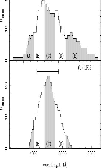
Figure 1.— Histograms of the data. The horizontal bar above the histograms shows the length of a Ly$\alpha$ forest spectrum with a midpoint at $z=2.7$. Shading marks the boundaries of the different redshift subsamples (see Table 1).

Table 1 The data subsamples.

Subsample	HIRES	HIRES	LRIS	LRIS
	$\langle z\rangle$	length	$\langle z\rangle$	length
		(${\rm\;km\;s^{-1}}$)		(${\rm\;km\;s^{-1}}$)
A	2.13	180000
B	2.47	389000	2.47	367000
C	2.74	375000	2.74	469000
D	3.03	255000	3.02	199000
E	3.51	278000
Fiducial	2.72	1016000	2.72	1049000

2.1. HIRES sample

The HIRES data were obtained as part of the effort to measure the mean cosmic baryon density $\Omega_{b}h^{2}$ by comparing the ratio of deuterium to hydrogen with the predictions of primordial nucleosynthesis (e.g., Tytler, Fan & Burles 1996; Burles & Tytler 1997, 1998, Burles, Kirkman & Tytler 1999). The reader is referred to these papers, as well as Kirkman & Tytler (1997), for details of observational techniques and data reduction procedures.

The sample used here consists of 30 Keck HIRES spectra, with QSO emission redshifts ranging from 2.19 to 4.11. The resolution is $8{\rm\;km\;s^{-1}}$ FWHM, and the spectra have been rebinned onto $2.1{\rm\;km\;s^{-1}}$ pixels. A Legendre polynomial continuum was fit to the echelle orders, using the IRAF task CONTINUUM, before they were combined to form a continuous spectrum. Averaging over all spectra, the mean $1\sigma$ uncertainty in the flux values of pixels relative to the continuum in the Ly$\alpha$ forest region is $4\%$.

The region that we use from each spectrum spans the wavelength range from Ly$\beta$ to 5000 ${\rm\;km\;s^{-1}}$ blueward of Ly$\alpha$ (to avoid the effect of any ionizing radiation arising from close proximity to the quasar). We show the redshift distribution of these Ly$\alpha$ forest data in Figure 1a, where we can see that redshifts from 1.6 to 4.1 are represented and that the peak in the histogram lies between $z=2.5$ and $z=3$. We have divided the dataset into different redshift subsamples, which are marked on Figure  1a and summarized in Table  1. The boundaries between the subsamples are at $z=2.3,2.6,2.9$, and $3.2$. The bulk of our analysis will be performed on a fiducial sample, which is the sum of data in subsamples B,C and D. This fiducial sample comprises the bulk of the data, and it has a relatively small redshift range in order to minimize the effects of evolution internal to the sample. It is centered roughly on the peak of the $z$ distribution, and the fiducial HIRES sample is comparable in size and mean redshift to the full LRIS sample discussed below.

                                                                            

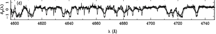
Figure 2.— Determination of $\delta_{F}(\lambda)$, for the quasar Q1017+1055. (a) LRIS spectrum (wiggly line), the continuum fitted over 100Å regions (upper smooth curve), and the spectrum smoothed with a 50Å Gaussian (lower smooth curve). (b) Fluctuations $\delta_{F}(\lambda)$ derived using the continuum fitted spectrum and the smoothed spectrum. The continuum fitted curve is slightly higher where the two are distinguishable. (c) Fluctuations $\delta_{F}(\lambda)$ from the HIRES spectrum of Q1077+1055. (d) A zoom of the central 150Å showing the two variations of the LRIS spectrum, the HIRES spectrum, and (grey curve) the HIRES spectrum smoothed to the resolution of the LRIS data.

2.2. LRIS sample

Large aperture telescopes are commonly used to probe to faint magnitudes with long exposures. Another possible application of their light gathering power is to build up a large sample of shallower exposures. This sort of approach is useful for the statistical study of large-scale structure, where it is important to minimize “cosmic variance.” In choosing the present LRIS data sample, our intention was to use the Keck telescope to carry out a quick survey comprising a relatively large number of quasar spectra. Because a high signal-to-noise ratio is not necessary for flux clustering measurements [at least for scales $\lesssim 0.1({\rm km\;s}^{-1})^{-1}$; see CWKH, and §3.3], it is possible to obtain useful spectra of bright $z\sim 3$ quasars with a few minutes integration time.

Because of the limited blue response of the instrument detectors, we were restricted to quasar targets with $z>2.7$. These were drawn from the quasar catalogue of Veron-Cetty & Veron (1998), and chosen to be as bright as possible. Of our targets, we were able to obtain spectra for 23, objects with V magnitudes ranging from 15.8 to 18.7, with the majority between 17.0 and 18.0. The highest redshift quasar in our sample is at $z=3.37$ and the lowest at $z=2.75$. The histogram of regions in the Ly$\alpha$ forest (running from Ly$\beta$ emission to 20 Å blueward of Ly$\alpha$ emission) is shown in Figure  1b. Our fiducial LRIS Ly$\alpha$ forest sample comprises all the LRIS data from $z=2.3$ to $z=3.2$. Our fiducial flux statistics will be measured by combining results from this sample and the HIRES data sample that covers the same redshift range. We have also subdivided the data to make subsamples with the same redshift boundaries as those of HIRES subsamples B,C, and D. Details are given in Table  1. Four of the quasars are also in the HIRES dataset and were used for comparison purposes (see below and §3.3).

The grating used for the LRIS observations was ruled with 900 lines/mm, with the blaze at 5500 Å. The FWHM resolution of the data was 2 Å, sampled with 0.85 Å  pixels. The data were taken on Dec. 10, 1998, with some spectra also taken during director’s observing time in Jan. 1999 and Feb. 1999. The integration times were between 10 and 30 minutes per object. Data reduction was carried out using standard IRAF packages for longslit spectroscopy. The signal-to-noise ratio of the resulting spectra varies between 10 and 50, with the majority having S/N of $\sim 40$ per pixel. Figure 2 (discussed below) displays a typical example from our LRIS spectra.

In our analysis of flux statistics, we will be interested in the mean flux $\langle F\rangle$ and the fluctuations about the mean $\delta_{F}(\lambda)\equiv F(\lambda)/\langle F\rangle-1$. We use $F(\lambda)$ to denote the transmitted flux, i.e., the ratio of the flux at a given wavelength $\lambda$ to the unabsorbed quasar continuum flux at $\lambda$. In order to find $F(\lambda)$, and hence $\langle F\rangle$, it is necessary to make an estimate of the unabsorbed continuum level. The quantity $\delta_{F}(\lambda)$ is much less sensitive to the exact assumed continuum level, as $\langle F\rangle$ has already been divided out. In the present paper, we will not attempt to make accurate determinations of $\langle F\rangle$ from our data. Instead, we will use $\langle F\rangle$ results from the literature and show how our results (for example for the amplitude of the matter power spectrum) would change for given future determinations of $\langle F\rangle$.

In order to calculate $\delta_{F}(\lambda)$, we have two choices. The first is to estimate a continuum level by fitting a line that passes through apparently unabsorbed regions of the spectrum. This has already been done in a semi-automated way for the HIRES data as described in §2.1 (see also Burles & Tytler 1998). For the LRIS data, which has much lower spectral resolution, our $\delta_{F}(\lambda)$ results are more likely to be sensitive to the continuum fitting technique used. We therefore compare two techniques applied to the LRIS data. The first is the automated technique described in CWPHK. This involves fitting a third-order polynomial through the datapoints in a given length of spectrum, rejecting points that lie 2$\sigma$ below the fit line, and iterating until convergence is reached. We implement this procedure using 100 Å fitting segments.

The second method for estimating $\delta_{F}(\lambda)$ is to calculate the mean flux level of the spectrum directly, rather than first fitting the continuum to scale unabsorbed flux to $F=1$. The mean level must be estimated from a region much larger than the length scales for which we are interested in measuring variations in $\delta_{F}(\lambda)$. This can be done either by fitting a low order polynomial to the spectrum itself (Hui et al. 2000) or by smoothing the spectrum with a large radius filter. We do the latter, using a 50 Å Gaussian filter. The value of $\delta_{F}(\lambda)$ is then given by $C(\lambda)/C_{S}(\lambda)-1$, where $C(\lambda)$ is the number of counts in the spectrum at a wavelength $\lambda$ and $C_{S}(\lambda)$ is the smoothed number of counts.

Figure 2 illustrates these two methods of determining $\delta_{F}(\lambda)$. Figure 2a shows the LRIS spectrum of the $z=3.16$ quasar Q107+1055, along with the fitted continuum (upper smooth curve) and the 50Å smoothed spectrum (lower smooth curve). Figure 2b compares $\delta_{F}(\lambda)$ estimated using the fitted continuum and using the smoothed spectrum. The two methods yield nearly indistinguishable results, with small differences appearing in regions where the spectrum is apparently close to the unabsorbed continuum. Figure 2c shows $\delta_{F}(\lambda)$ from the (continuum-fitted) HIRES spectrum of Q107+1055. Figure 2d blows up the central 150Å of the spectrum, superposing the two LRIS $\delta_{F}(\lambda)$, the HIRES $\delta_{F}(\lambda)$, and the HIRES $\delta_{F}(\lambda)$ smoothed to the spatial resolution of the LRIS data. The smoothed HIRES spectrum matches the LRIS spectrum almost perfectly, providing further evidence of the robustness of the $\delta_{F}(\lambda)$ determination. In §3.3 we will compare the HIRES and LRIS flux power spectra for the four quasars common to both samples. We will also show that the two methods of determining $\delta_{F}(\lambda)$ from the LRIS spectra yield similar power spectrum results. We will adopt the smoothed spectrum method as our standard, since it does not involve splitting a spectrum into discrete segments and is simpler to implement in a robust manner.

As in CWPHK, we scale the individual pixel widths in the spectra to the size they would have at the mean redshift of the sample in question. In the present work, we do this assuming that the evolution of $H(z)$ follows that in an EdS universe, which should be a good approximation at these high redshifts (see also M00). We also follow Rauch et al. (1997) and CWPHK in scaling the optical of pixels depths by a factor of $(1+z)^{4.5}$ to the mean $z$ of the sample, in order to mitigate the effects of evolution. We have done this only for the HIRES data, since for the LRIS data we are already calculating $\delta_{F}(\lambda)$ with respect to the local mean. The effects of both of these rescalings on the flux power spectrum are investigated in §3.3.

3. Statistics of the transmitted flux

In the fluctuating intergalactic medium (IGM) view of the Ly$\alpha$ forest described in §1, the most natural statistical descriptors of the forest are those that treat each spectrum of transmitted flux as a continuous one-dimensional field, rather than a collection of lines. Many such statistics have been discussed in the literature, including the one-point flux probability distribution, the threshold-crossing frequency, and the filling factor of saturated regions (e.g., Miralda-Escudé et al. 1996, 1997; Cen 1997; Croft et al. 1997a; Rauch et al. 1997; Croft & Gaztañaga 1999; Theuns, Schaye, & Haehnelt 1999; Weinberg et al. 1999b; M00). These measures are analogous to, and in some cases borrowed from, those used to study large-scale structure in the galaxy distribution. They encode information about the underlying matter distribution and about the temperature and physical state of the IGM.

In this section we focus on the statistics that are most relevant to determination of the matter power spectrum, namely the flux power spectrum and its Fourier transform, the flux correlation function. As mentioned in §1, the inference of the matter power spectrum depends on the value of the mean transmitted flux $\langle F\rangle$, or, equivalently, the effective mean optical depth

$$\overline{\tau}_{\rm eff}\equiv-\ln\langle F\rangle.$$ (3)

We will not undertake a direct measurement of $\overline{\tau}_{\rm eff}$ here, but we will examine a statistic, the flux filling factor, that provides an indirect handle on $\overline{\tau}_{\rm eff}$. Although determination of the matter power spectrum is our long-term goal, the measurements of flux statistics in this section can also stand as direct tests of theoretical predictions for the Ly$\alpha$ forest, derived from numerical simulations or analytic approximations. The flux correlation function and flux power spectrum have been measured for an independent sample of Keck HIRES spectra by M00.

                                                                            

Figure 3.— (a) The filling factor FF of regions below a flux threshold of 0.5, computed as a function of redshift from the HIRES data. Error bars ($1\sigma$) are calculated using a jackknife estimator. (b) Confidence intervals (68%, 95%, 99.7%) on parameters $c_{1}$ and $c_{2}$, determined by fitting the functional form FF$=c_{1}\exp{(c_{2}z)}$ to the data points in (a). Best fit values (cross) are $c_{1}=0.0291$, $c_{2}=0.719$. In (a), the shaded bands show the region corresponding to the 68% confidence interval on $(c_{1},c_{2})$.

3.1. Filling factor

In terms of the discussion in §1, the role of $\overline{\tau}_{\rm eff}$ in our analysis is to allow us to determine the constant $A$ in equation (2), given a model of the density fluctuations $(\rho/{\overline{\rho}})$ obtained from N-body simulations. However, observational determinations of $\overline{\tau}_{\rm eff}$ are sensitive to the details of continuum fitting because a significant fraction of the mean opacity arises in long stretches of weak absorption close to the unabsorbed continuum. The filling factor FF, the fraction of a spectrum that lies below a specified flux threshold, offers another diagnostic for $A$ that is less sensitive to the continuum level, and we will use it as a consistency check on our adopted value of $\overline{\tau}_{\rm eff}$. While the filling factor of saturated regions ($F\approx 0$) would be the least sensitive to continuum determination, it is also not sufficiently sensitive to $A$ to be useful for our purposes. Instead, we measure the filling factor of regions with $F\leq 0.5$, which is likely to be almost as insensitive to continuum uncertainty (see, e.g., figure 2b, and figure 5 of Nusser & Haehnelt 2000).

For this statistic, we use the HIRES data only, as we are interested in unsmoothed spectra. We split the data into 12 redshift bins of width $\Delta z=0.2$, spanning $z=1.7$ to $z=4.1$. We calculate the FF for $F=0.5$ for each redshift range and plot the results in Figure 3a, as a function of redshift. The error bars are computed using a jackknife estimator (Bradley 1982), which we will employ for error estimation on other statistics as well. For a statistic $X$ estimated from a data sample, the jackknife estimate of the $1\sigma$ uncertainty on $X$ is obtained by dividing the sample into $N$ subsamples and computing $\sigma=\left[\sum_{i=1}^{N}\left(X_{i}-\widehat{X}\right)^{2}\right]^{1/2}$, where $\widehat{X}$ is the estimate from the full data sample and $X_{i}$ is the value estimated by leaving out subsample $i$. For Figure 3a, we split the data for each redshift bin into $N=5$ subsamples to estimate the error bars.

A rapid increase in FF with redshift can be seen from the plot. By $z\simeq 4.0$, half of each spectrum lies below the $F=0.5$ level, as opposed to $\simeq 10\%$ at $z=1.8$. In order to present the results in a form which is easy to use, we carry out a $\chi^{2}$ fit to the function FF$=c_{1}\exp{(c_{2}z)}$. The best fit line is shown on Figure 3a. We find that $c_{1}=0.0291\pm 0.0006$ and $c_{2}=0.719\pm 0.008$ (these are $1\sigma$ errors for the parameters taken individually). The $\chi^{2}$ for these parameters is 6.9 (for 10 degrees of freedom). The errors on $c_{1}$ and $c_{2}$ are highly correlated, as can be seen in panel (b) of Figure  3. The shaded band of panel (a) shows the values of FF$(z)$ that result from varying the parameters $c_{1}$ and $c_{2}$ so that they sample the entire joint $68\%$ confidence interval on their values. Using this fit information gives fractional errors on FF of $4.9\%$ at $z=2$, $2.0\%$ at $z=3$ and $5.8\%$ at $z=4$. At the redshift of the fiducial sample ($z=2.72$), the error is $2.1\%$ and the FF is 0.205. Of course these error values are derived from the fit, and their use implies the assumption that the FF is changing smoothly with $z$ in accordance with the shape given by the fit. This assumption has been used by others for studying the evolution of the mean flux level with $z$ (e.g., Press, Rybicki & Schneider 1993, hereafter PRS).

3.2. Flux correlation function

The flux correlation function, $\xi_{F}(r)$, is a simple statistic to calculate. Its usefulness has been emphasized by Zuo & Bond (1994) and Cen et al. (1998), amongst others, and $\xi_{F}(r)$ has been measured from a sample of eight Keck HIRES spectra by M00. We will also use it for a consistency check on our 3-d $P(k)$ inversion, in §3.3.3 below. We estimate $\xi_{F}(r)$ from our quasar data using the estimator $\xi_{F}(r)=\langle\delta_{F}(x)\delta_{F}(x+r)\rangle$. We present results for the fiducial sample in Table 2. The errors were again calculated using a jackknife estimator, and although we only give the diagonal terms in the covariance matrix, the full matrix (which has large off-diagonal terms) is available from the authors on request. In Table 2, we have averaged the results from the LRIS and HIRES samples on large scales ($r>250{\rm\;km\;s^{-1}}$), where the finite LRIS resolution is not important. On smaller scales, only the HIRES results are used. Table 6 (see Appendix) gives $\xi_{F}(r)$ for the different redshift subsamples.

Table 2 The flux correlation function, $\xi_{F}(r)$, for the fiducial sample ($\langle z\rangle=2.72$).

r	$\xi_{F}(r)$
(${\rm\;km\;s^{-1}}$)
11.4	$0.184\pm 0.007$
14.9	$0.174\pm 0.007$
19.4	$0.172\pm 0.008$
25.3	$0.157\pm 0.007$
32.9	$0.144\pm 0.007$
42.9	$0.127\pm 0.007$
56.0	$0.104\pm 0.006$
72.9	$(8.5\pm 0.6)\times 10^{-2}$
95.0	$(6.6\pm 0.5)\times 10^{-2}$
124	$(5.0\pm 0.5)\times 10^{-2}$
161	$(3.7\pm 0.4)\times 10^{-2}$
210	$(2.7\pm 0.4)\times 10^{-2}$
274	$(1.9\pm 0.3)\times 10^{-2}$
357	$(1.4\pm 0.3)\times 10^{-2}$
466	$(9.4\pm 2.1)\times 10^{-3}$
607	$(6.2\pm 2.2)\times 10^{-3}$
791	$(4.1\pm 2.1)\times 10^{-3}$
1030	$(2.6\pm 2.0)\times 10^{-3}$
1340	$(-7.9\pm 17.7)\times 10^{-4}$
1750	$(-1.8\pm 1.6)\times 10^{-3}$

Figure 4.— The flux correlation function of the various data subsamples. The solid line in each case is the fiducial combined sample, with the length scaled so that the comoving lengths stay the same in an EdS model. The multiplicative factor used is $[(1+z_{i})/(1+z_{F})]^{1/2}$, where $z_{i}$, $z_{F}$ are the mean redshifts of subsample $i$ and the fiducial sample respectively. Filled circles represent the HIRES data and open circles the LRIS data. Error bars have been omitted from the latter, for clarity.

We plot $\xi_{F}(r)$ for the different redshift subsamples in Figure 4, with results for the fiducial sample shown as the solid curve in each panel. There is a measurable clustering signal out to $r\sim 2000{\rm\;km\;s^{-1}}$ (note that we are plotting both axes with a log scale). In the same way that the flux power spectrum in simulations appears to have much the same shape as the (linear) matter power spectrum (e.g., CWKH), we expect the shape of $\xi_{F}(r)$ to reflect that of the underlying matter correlation function, at least over some range of scales. A comparison of $\xi(r)$ for flux and mass has been carried out by Cen et al. (1998).

On the largest scales, and particularly at high redshift, $\xi_{F}(r)$ could in principle be influenced by UV background fluctuations or by continuum fitting errors. However, Figure 4 implies that any such effects are not strong, since the shape of $\xi_{F}(r)$ in the different panels does not appear to change significantly from one redshift to the next. This consistency is expected if $\xi_{F}(r)$ is mainly determined by the underlying matter distribution, but it seems coincidental if the fluctuations that are quantified by $\xi_{F}(r)$ are generated by some other mechanism. However, the possibility that UV background fluctuations could reproduce this behaviour merits further study, since, for example, clustered sources and absorbing material could conceivably yield a $\xi_{F}(r)$ related to that of the matter distribution. For work that shows that this is unlikely to occur on the scales of interest to us here, see, e.g., Zuo (1992) and CWPHK.

Predicting the evolution of $\xi_{F}(r)$ in a given cosmological model involves a combination of change in length units, growth of matter clustering, and evolution of the mean opacity. We leave such predictions to future work, which should also investigate the consistency of higher-order statistics of the flux with the FGPA predictions. For the time being, we note that the amplitude of $\xi_{F}(r)$ decreases as we move to lower redshift, as the rapidly decreasing value of $\overline{\tau}_{\rm eff}$ counteracts the effect of gravitational clustering. This means that a good knowledge of $\overline{\tau}_{\rm eff}$ is needed to make measurements of the amplitude of matter fluctuations (see §5.4). On small scales ($r\lesssim 200{\rm\;km\;s^{-1}}$), the shape of $\xi_{F}(r)$ reflects the broadening of individual absorption features by Hubble flow, peculiar velocities, and thermal motions (Zuo & Bond 1994; Hernquist et al. 1996).

3.3. Flux power spectrum

3.3.1 Definitions

To compute the one-dimensional flux power spectrum, $P_{F,1D}(k)$, we must decompose the absorption spectra into Fourier modes and measure their variance as a function of wavenumber. In CWKH and CWPHK, we accomplished this task using a Fast Fourier Transform (FFT). This approach requires mapping the spectra onto equally spaced bins using spline interpolation. M00 calculated $P_{F,1D}(k)$ by an alternative technique, the Lomb periodogram, which does not require the assumption of periodic boundary conditions and which works for unequally spaced bins (see Press et al. 1992). In the present paper we also adopt this approach to derive our fiducial results (using the Lomb code from Press et al. 1992). We compare results obtained using this method and the FFT below.

The power spectrum along a line of sight is an integral over the power spectrum of the corresponding 3-dimensional field (Kaiser & Peacock 1991). Since we are ultimately interested in the 3-dimensional matter power spectrum, we want to work with the corresponding property of the flux. We will define the 3D flux power spectrum $P_{F}(k)$ by the relation

$$P_{F}(k)=-\frac{2\pi}{k}\frac{d}{dk}P_{F,1D}(k),$$ (4)

so that $P_{F}(k)$ is the power spectrum of the 3D “flux field” that would have a line-of-sight power spectrum $P_{F,1D}(k)$ if it were isotropic. In practice, peculiar velocities and thermal motions make the flux field anisotropic (Hui 1999; McDonald & Miralda-Escudé 1999), but this anisotropy has relatively little impact on the inferred matter power spectrum over the scales provided by our analysis, and our procedure for estimating the matter $P(k)$ will account for it automatically. In place of $P_{F}(k)$, we will show in our plots the quantity

$$\Delta^{2}_{\rm F}(k)\equiv\frac{1}{2\pi^{2}}k^{3}P_{F}(k),$$ (5)

which is the contribution to the variance of the flux from an interval $d\ln k=1$. The reader should note that this definition of $\Delta^{2}_{\rm F}(k)$ differs from that in CWKH and CWPHK by the factor $(1/2\pi^{2})$. Also, with this convention our definition of $P_{F,1D}(k)$ is larger than that given in M00 by a factor of 2.

3.3.2 Tests for systematic errors

                                                                            

Figure 5.— Dependence of the flux power spectra $\Delta^{2}_{\rm F}(k)$ on spectral resolution and continuum fitting method. (a) We use the four quasar spectra common to the LRIS and HIRES samples and show the power spectrum derived from the HIRES observations (circles) and the LRIS observations with 50Å Gaussian smoothing for determination of the mean level (triangles). Open circles correspond to negative values of $\Delta^{2}_{\rm F}(k)$. Lower panel shows the difference from the mean of the two power spectra in units of the mean. Error bars represent $1\sigma$ jackknife errors derived from the four spectra. (b) Comparison of LRIS results using two methods of continuum fitting, smoothing with a 50Å Gaussian (triangles) and fitting over a 100Å region with a 3rd order polynomial (circles). Here we use all 23 LRIS spectra in the LRIS sample, and the error bars represent jackknife errors derived by partitioning those 23 spectra into 50 subsets of equal length (see §3.3.2).

We first compare $\Delta^{2}_{\rm F}(k)$ measured from the four quasars for which we have both LRIS and HIRES spectra. These are Q0636+6801, Q0940-1050, Q1017+1055, and Q1107+4847. In the top panel of Figure 5a, we show $\Delta^{2}_{\rm F}(k)$ measured from the LRIS spectra, where $\delta_{F}(r)$ was calculated using the ($50$ Å) Gaussian smoothing method for finding the local mean flux. We also show the HIRES results. In the lower panel, we plot the difference between the two measurements of $\Delta^{2}_{\rm F}(k)$, in units of the mean $\Delta^{2}_{\rm F}(k)$ for the two sets of spectra. The error bars were calculated by applying a jackknife estimator to the four spectra in each set. We can see that there are some differences in detail between the two sets of $\Delta^{2}_{\rm F}(k)$ results, but they appear to be consistent within the errors, at least on large scales. On small scales, the LRIS results are systematically lower, as we expect because of the lower resolution of the spectra. We shall see later (§3.3.4) that smoothing the spectra can potentially have effects on the inversion from 1D to 3D clustering on fairly large scales. As a test of any systematic differences, we have tried a least-squares fit of a horizontal straight line to the first ten points in the lower panel of Figure 5a. We find that any uniform bias on these scales is consistent with zero within the errors (we find $0.08\pm 0.11$ at 1 $\sigma$).

In Figure 5b, we carry out a similar test of the two different ways of analyzing the LRIS spectra, measuring $\delta_{F}(r)$ using a fitted continuum versus smoothing the spectrum to define the mean. Because we are just using the LRIS data for this, we carry out the test using all 23 spectra. A horizontal fit to the first 10 points yields a mean bias between the two of $-0.005\pm 0.030$ at $1\sigma$.

                                                                            

Figure 6.— Comparison of the 1D flux power spectrum from M00 (open circles) and from our HIRES spectra (filled circles), for subsamples covering the redshift range $z=2.67$ to $z=3.39$. The mean redshift of the M00 data is 3.0 and that of our subsample 2.98. Because of differing Fourier conventions, we have multiplied the M00 results by a factor of 2.

Previously, M00 presented $P_{F,1D}(k)$ measured from a sample of Keck HIRES spectra. In order to compare our results to theirs, we have prepared a sample of our HIRES data that has the same redshift boundaries as one of the data samples in M00, $z=2.67$ to $z=3.39$. The M00 sample with these boundaries has $\langle z\rangle=3.0$, and ours has $\langle z\rangle=2.98$. The M00 spectra are a sample of eight with extremely high signal-to-noise ratio, and which have a FWHM of $6.6{\rm\;km\;s^{-1}}$, binned into $2.4{\rm\;km\;s^{-1}}$ pixels. The equivalent of $\sim 2.5$ full spectra contribute to the M00 results for the redshift range we use here, compared to $\sim 13$ (total length $6.4\times 10^{5}{\rm\;km\;s^{-1}}$) for the comparison sample of our data.

In Figure 6, we show $P_{F,1D}(k)$ from M00 and our comparison sample. We can see that on scales $k<0.1({\rm km\;s}^{-1})^{-1}$, there is good agreement between the two measurements, and the larger number of spectra in our sample is reflected in a smoother curve and smaller error bars. We have calculated these error bars with a jackknife estimator, as we did for the $\xi_{F}$ results (see §3.2), except that when partitioning the data we use 50 subsets. The error bars on the M00 points come from bootstrap resampling, which should yield similar results to the jackknife technique. In Figure 6, we show only scales $k<0.1({\rm km\;s}^{-1})^{-1}$, as on smaller scales, we find that the results diverge. This is likely to be due to the lower S/N of our data. We investigate the effects of S/N on $\Delta^{2}_{\rm F}(k)$ below. The M00 data are also of slightly higher resolution (our data have FWHM of $8.0{\rm\;km\;s^{-1}}$, $20\%$ broader than M00).

Although we would like to have as large a dynamic range possible in our flux power spectrum measurements, $k=0.1({\rm km\;s}^{-1})^{-1}$ represents the scale below which M00 have found that their results are sensitive to whether known metal lines are removed or not. Since we do not attempt this procedure, which would introduce additional uncertainties, we are limited to points with $k<0.1({\rm km\;s}^{-1})^{-1}$ even without consideration of S/N and spectral resolution.

                                                                            

Figure 7.— Dependence of $\Delta^{2}_{\rm F}(k)$ on S/N ratio of the quasar spectra. Open circles show the 3D flux power spectrum from M00, and filled circles show the measurement from our HIRES subsample with the same redshift boundaries. Stars and squares show $\Delta^{2}_{\rm F}(k)$ derived from the half of the HIRES subsample with highest and lowest S/N, respectively.

In order to test the effect of noise on $\Delta^{2}_{\rm F}(k)$, we split the M00 comparison sample into two. Spectra with a mean $1\sigma$ error in $F$ per pixel $>0.040$ are in the high noise subsample. This subsample has a mean error per pixel of $0.074$ and $\langle z\rangle=3.0$. The low noise subsample, comprising the rest of the data, has a mean noise per pixel of $0.026$ and $\langle z\rangle=2.96$. The total lengths of spectra in the high and low noise subsamples are approximately equal. We show the $\Delta^{2}_{\rm F}(k)$ results in Figure 7, together with $\Delta^{2}_{\rm F}(k)$ for the M00 data. The noise level of the data (which is dominated by Poisson distributed photon noise) does affect the level of power on scales $k\gtrsim 0.15({\rm km\;s}^{-1})^{-1}$. However, we will limit our measurement of the matter $P(k)$ to scales $k<0.05({\rm km\;s}^{-1})^{-1}$ anyway because of separate uncertainties related to the flux to mass reconstruction. On these scales, any systematic bias associated with S/N is small, with low S/N points being slightly lower for $k\gtrsim 0.03({\rm km\;s}^{-1})^{-1}$.

                                                                            

Figure 8.— Tests of different ways of computing the power spectrum and of scaling the data. Open circles show the 3D flux power spectrum of M00 and filled circles the results of our standard treatment, for the comparison HIRES subsample with the same redshift boundaries. For these data points, and for those in the rest of the paper, we scale pixel sizes and optical depths to the sample mean redshift and estimate $P_{F}(k)$ using the Lomb periodogram. Stars show the result with no scaling to the mean redshift. Squares show the result of scaling the data but estimating $P_{F}(k)$ with an FFT instead of the Lomb periodogram.

In Figure 8 we test details of the power spectrum estimation method, again using the HIRES subsample designed for comparison to M00. Filled circles, repeated from Figure 7, show results of our standard treatment. Stars show $\Delta^{2}_{\rm F}(k)$ computed using the same power spectrum estimator (the Lomb periodogram) but no scaling of pixel sizes or optical depths to the mean redshift (see §2.2). There appear to be only small and non-systematic differences between these two treatments. The differences are even smaller when we compare the fiducial results to those obtained from FFT measurements of the power spectrum (squares). We are therefore confident that no problems have been introduced by the use of an FFT in previous papers. However, the Lomb periodogram is better motivated, so we adopt it here.

Table 3 The flux power spectrum, for the fiducial sample ($\langle z\rangle=2.72$).

k	$P_{F,1D}(k)$	$P_{F}(k)$
$({\rm\;km\;s^{-1}})^{-1}$	$({\rm\;km\;s^{-1}})^{-1}$	$({\rm\;km\;s^{-1}})^{-3}$
0.00199	$41.1\pm 4.4$	$(2.50\pm 3.19)\times 10^{7}$
0.00259	$36.3\pm 3.6$	$(1.97\pm 1.15)\times 10^{7}$
0.00337	$29.7\pm 2.8$	$(1.26\pm 0.54)\times 10^{7}$
0.00437	$24.8\pm 2.1$	$(3.45\pm 2.32)\times 10^{6}$
0.00568	$25.5\pm 1.6$	$(1.45\pm 0.96)\times 10^{7}$
0.00738	$21.8\pm 1.6$	$(2.31\pm 0.43)\times 10^{7}$
0.00958	$18.7\pm 1.2$	$(8.79\pm 1.57)\times 10^{5}$
0.0124	$15.1\pm 0.9$	$(5.17\pm 0.75)\times 10^{5}$
0.0162	$12.0\pm 0.6$	$(3.01\pm 0.53)\times 10^{5}$
0.0210	$8.69\pm 0.33$	$(1.64\pm 0.23)\times 10^{5}$
0.0272	$6.30\pm 0.27$	$(7.77\pm 0.68)\times 10^{4}$
0.0355	$4.00\pm 0.14$	$(4.07\pm 0.27)\times 10^{4}$
0.0461	$2.28\pm 0.12$	$(1.72\pm 0.08)\times 10^{4}$
0.0598	$1.17\pm 0.06$	$6340\pm 410$
0.0777	$0.561\pm 0.036$	$2050\pm 110$
0.101	$0.239\pm 0.021$	$600\pm 35$
0.131	$0.114\pm 0.015$	$135\pm 9$
0.170	$0.0712\pm 0.013$	$28.5\pm 2.7$
0.221	$0.0533\pm 0.013$	$8.14\pm 0.81$
0.287	$0.0400\pm 0.010$	$3.74\pm 0.86$

3.3.3 Test of inversion from the 1D to the 3D flux power spectrum

We would also like to test our method of deriving the 3D flux power spectrum from the 1D flux power spectrum, since one might worry that the differentiation required by equation (4) leads to biases in the presence of noise. A simple test, illustrated in Figure 9, is to check that $P_{F}(k)$ and $\xi_{F}(r)$ form the expected Fourier transform pair:

$$\xi_{F}(r)=\frac{1}{(2\pi)^{3}}\int^{\infty}_{0}P_{F}(k)\frac{\sin{(kr)}}{kr}4\pi k^{2}dk,$$ (6)

$$P_{F}(k)=\int^{\infty}_{0}\xi_{F}(r)\frac{\sin{(kr)}}{kr}4\pi r^{2}dr.$$ (7)

Points in the upper panel show $\Delta^{2}_{\rm F}(k)$ estimated from our full fiducial sample (B+C+D, HIRES and LRIS), with our standard methodology. The solid curve shows the Fourier transform of the flux correlation function (eq. 7), where we have used the linear power spectrum of the LCDM model described in §4.2 to extrapolate $\xi_{F}(r)$ beyond the observed $r$ limits. The dashed curve shows the Fourier transform when the integral is simply truncated at the observational limits $r_{\rm min}$ and $r_{\rm max}$. The lower panel of Figure 9 displays an analogous comparison between the directly measured $\xi_{F}(r)$ and the Fourier transform (eq. 6) of $P_{F}(k)$.

                                                                            

Figure 9.— (a) Comparison of the flux power spectrum measured directly from the fiducial (B+C+D, $\langle z\rangle=2.72$) sample (points) with that estimated by carrying out a Fourier transform of the flux correlation function of the fiducial sample (lines). The different lines show two different ways of extrapolating the measured $\xi_{F}(r)$ when carrying out the numerical integral. The solid line shows an extrapolation which uses the LCDM shape, and the dashed line uses a truncated form for $\xi_{F}(r)$ (see text). (b) Comparison of the flux correlation function $\xi_{F}(r)$ measured directly from the fiducial sample (points) with that estimated by carrying out a Fourier transform of the flux power spectrum of the fiducial sample (lines). Again the lines show two different ways of carrying out the extrapolation, solid being LCDM and dashed a truncated $P_{F}(k)$ (see text).

These comparisons show that the two totally different methods for inferring three-dimensional clustering give very similar results. There is also little impact on Fourier transform estimates of $P_{F}(k)$ or $\xi_{F}(r)$ from scales where we have no direct measurements. The agreement found in Figure 9 justifies our earlier assertion that equation (4) defines a quantity close to the power spectrum of the three-dimensional “flux field,” despite the presence of some redshift-space anisotropy (see Hui 1999; McDonald & Miralda-Escudé 1999). We adopt this approach in preference to the inversion of $\xi_{F}(r)$, which is rather difficult to handle numerically, particularly on the smallest scales.

3.3.4 Smoothing bias

There is another, somewhat subtle effect that influences the inversion from 1D to 3D when using low resolution spectra. Finite spectral resolution smooths the 1D power spectrum by convolution with the square of the instrument response function. Because the 3D power spectrum is obtained by differentiation (eq. 4), this steepening of the 1D power spectrum artificially boosts the amplitude of the 3D power spectrum, even on scales that are significantly larger than the smoothing scale.

                                                                            

Figure 10.— Test of “smoothing bias”, the effect of smoothing a spectrum (for example due to finite spectral resolution) on the inversion from 1D to 3D. Solid lines show the linear theory power spectra $\Delta^{2}(k)$ of CDM models with shape parameter (see §4.2) $\Gamma=0.05$ (thick) and $\Gamma=0.5$ (thin). Dashed lines show the result of deriving the 3D power spectrum from the corresponding 1D power spectra smoothed with a Gaussian filter of $\sigma=50{\rm\;km\;s^{-1}}$, approximately equivalent to 2Å FWHM spectral resolution. Dotted lines show the result for $\sigma=150{\rm\;km\;s^{-1}}$ (6Å FWHM) smoothing. The derived $\Delta^{2}(k)$ is suppressed on small scales by smoothing, but it is boosted on intermediate scales because of the differentiation required to go from 1D to 3D.

We show the effect of this “smoothing bias” on linear theory power spectra in Figure 10. Here we have multiplied $P_{F,1D}$ by a Gaussian filter, to simulate observational smoothing, then used equations (4) and (5) to find $\Delta^{2}_{\rm F}(k)$. We show results for two different power spectrum shapes, characterized by the shape parameter $\Gamma$ (see §4.2). The amount of bias depends on the shape, but the two we show are fairly close to the observed shape, at least on large scales, and the bias seen in both should be representative. We find that on the largest scale we observe, $2\times 10^{-3}({\rm km\;s}^{-1})^{-1}$, the boost in $\Delta^{2}_{\rm F}(k)$ with the 2 Å spectral resolution typical of our LRIS data is $3\%$, while for much lower resolution of 6 Å it would be $20\%$. This artificial amplification increases to a maximum of 14% for the smallest scale we make use of for the 2 Å case, and would be 32% for 6Å. On the very smallest scales, smoothing suppresses $\Delta^{2}_{\rm F}(k)$. On the scales where we use the LRIS data, $k<0.014({\rm km\;s}^{-1})^{-1}$, they contribute about half the signal of the fiducial sample, so with no correction we would expect a bias of $1.5\%-7\%$ on these scales. To remove this effect, we adjust the LRIS contributions to $P_{F}(k)$ using correction factors derived from the fractional differences between the lower curves in Figure 10; however, we limit the maximum correction to 10%, since the value close to the smoothing scale is sensitive to the assumed form of the input spectrum. Since the maximum corrections to $P_{F}(k)$ are only a few percent, the uncertainties in the corrections are much smaller than the $1\sigma$ error bars on the affected data points, which are $\gtrsim 15\%$. The agreement of $\Delta^{2}_{\rm F}(k)$ derived from HIRES and LRIS spectra of the same quasars (Figure 5), for which we applied no correction to the LRIS $\Delta^{2}_{\rm F}(k)$, is further evidence that smoothing bias is a minor issue in the context of this data set. However, it could be important for data of substantially lower spectral resolution. Because the degree of bias depends on the precise form of the spectral response function and on the shape of the underlying power spectrum, a rigorously accurate correction is difficult, and alternative analysis methods should be considered for lower resolution data.

3.3.5 The flux power spectrum and its covariance matrix

Figure 11 presents the principal results of this section, the flux power spectrum $\Delta^{2}_{\rm F}(k)$ of the fiducial sample and the various redshift subsamples. The values of $P_{F,1D}(k)$ and $P_{F}(k)$ for the fiducial sample are listed in Table 3, and the values of $P_{F,1D}(k)$ for the redshift subsamples are listed in Table 7 of the Appendix. We average the contributions of the LRIS and HIRES data on scales $k<0.014({\rm km\;s}^{-1})^{-1}$ for $\Delta^{2}_{\rm F}(k)$ and $k<0.006({\rm km\;s}^{-1})^{-1}$ for $P_{F,1D}(k)$, which is more strongly affected by the spectral resolution. We also average the $1\sigma$ error bars and divide them by $\sqrt{2}$. We do not account for the fact that four spectra appear in both samples, so our error bars on these large-scale datapoints may be systematically underestimated by as much as $\sim 1-\sqrt{49/53}=4\%$. We use only the HIRES data on smaller scales.

Figure 11.— The flux power spectrum of the various data subsamples. The solid line in each case is the fiducial combined sample, with the length scaled so that the comoving lengths stay the same in an EdS model. The filled points are the HIRES data and the open circles the LRIS data. Error bars have been omitted from the latter, for clarity.

                                                                            

Figure 12.— The covariance matrix of the flux power spectrum of the fiducial HIRES sample. The symbol area is proportional to $C_{ij}/(C_{ii}C_{jj})^{1/2}$, with negative elements shown by open symbols. The flux power spectrum values which correspond to this covariance matrix are given in Table 3. The elements span scales of 0.00199 $({\rm km\;s}^{-1})^{-1}$ (element 1) to 0.287 $({\rm km\;s}^{-1})^{-1}$ (element 20).

The error bars in Figure 11 and Tables 3 and 7 are computed using a jackknife estimator, with 50 data subsets in each case. Although the flux correlation function $\xi_{F}(r)$ has strongly covariant errors, we might expect the errors on the $\Delta^{2}_{\rm F}(k)$ data points to be close to independent, at least if they reflect the behavior of the linear matter power spectrum. M00 found that the covariance matrix of $P_{F,1D}(k)$ measured from their data is extremely noisy but consistent with the off-diagonal elements being zero.

Figure 12 illustrates the covariance matrix $C_{ij}$ of $\Delta^{2}_{\rm F}(k)$ for our fiducial HIRES data (with $\langle z\rangle=2.72$), again estimated by the jackknife technique. We have divided out the diagonal elements, so that the symbol area is proportional to $C_{ij}/(C_{ii}C_{jj})^{1/2}$. It is obvious from the plot that $C_{ij}$ is fairly close to diagonal, at least for the elements with $i$ and $j$ $\lesssim 13$. The matrix is also quite noisy, with the uncertainty on $C_{ij}$ increasing as we move towards small $i$ and $j$ (larger scales), where there are fewer modes to average over. On the smallest scales we find significantly positive non-diagonal elements. These scales are smaller than the smallest ones we shall be using to reconstruct the matter power spectrum. On larger scales some of the off-diagonal elements appear to be small but negative. This behavior was also seen in the CWPKH covariance matrix, and if it is statistically significant it is probably caused by the differencing needed to compute $P_{F}(k)$ from $P_{F,1D}(k)$. Given that the covariance matrix is noisy and that anti-covariance caused by negative elements would decrease error bounds, we will adopt the conservative position of using only the diagonal elements in our analysis of the matter power spectrum.

The error bars in Figure 11 are much larger than those on $\xi_{F}(r)$ in Figure 4 because in this case they are nearly uncorrelated. The shape of $\Delta^{2}_{\rm F}(k)$ remains roughly the same at all redshifts on large scales, while the relative amount of power on small scales appears to decrease with decreasing redshift, presumably due to increasing non-linearity and peculiar velocities. The overall amplitude of $\Delta^{2}_{\rm F}(k)$ drops towards lower redshifts, as for $\xi_{F}(r)$. This drop is driven by the decrease of $\overline{\tau}_{\rm eff}$ as the universe expands. We will show in §6.3 that, once the evolution of $\overline{\tau}_{\rm eff}$ is taken into account, these $\Delta^{2}_{\rm F}(k)$ results yield a marginal detection of the expected signature of gravitational growth of the underlying matter fluctuations.

4. From flux to mass: method

4.1. Overview

CWKH proposed a method for recovering the linear matter power spectrum $P(k)$ from measurements of the Ly$\alpha$ forest flux power spectrum, and CWPHK applied this method to a sample of 19 moderate resolution quasar spectra. The method that we use to recover $P(k)$ in this paper has evolved from that used by CWKH and CWPHK, but it is significantly better. Specifically, our current method is to assume that

$$P_{F}(k)=b^{2}(k)P(k)$$ (8)

and that the values of $b(k)$ can be calibrated using numerical simulations that are tuned to match the observed $\overline{\tau}_{\rm eff}$ and $P_{F}(k)$. In this language, the method used in CWKH and CWPHK assumed $b={\rm constant}$, and CWKH defined $P_{F}(k)$ from the “Gaussianized” flux rather than the flux itself. The $b={\rm constant}$ assumption is reasonably accurate on large scales, where, at least according to hydrodynamic simulations, the shape of the flux power spectrum is similar to that of the linear matter power spectrum. This similarity of shape is expected if the matter density and flux are related by a local transformation (see, e.g., Coles 1993; Gaztañaga & Baugh 1998; Scherrer & Weinberg 1998; M00 Appendix C), as they are in the Fluctuating Gunn-Peterson Approximation. However, the method adopted here is obviously more general, and it can account for the effects of redshift-space distortions, non-linear evolution, and thermal broadening, which change the shape of $P_{F}(k)$. This improvement in method is justified by the larger size and dynamic range of our current data set, since with the previous method the accuracy of our recovered $P(k)$ would be limited by the accuracy of the $b={\rm constant}$ approximation. As in the previous method, there are systematic uncertainties in the transformation from $P_{F}(k)$ to $P(k)$ because there are uncertainties in the parameter values to adopt for the calibrating simulations; we will discuss these systematic uncertainties in §5. Our current approach is, in some sense, intermediate between that of CWPHK, who determined the amplitude of $P(k)$ using simulations with the initial $P(k)$ shape inferred from the Ly$\alpha$ forest data themselves, and that of M00, who did not attempt an inversion of $P(k)$ but estimated $P(k)$ parameter constraints by scaling the predictions of a hydrodynamic simulation. However, our approach here also includes new features not present in either of these previous methods.

                                                                            

Figure 13.— Flowchart for matter power spectrum reconstruction.

The results of previous investigations (CWPHK; M00; Phillips et al. 2001) imply that the shape of the linear matter power spectrum $P(k)$ on Ly$\alpha$ forest scales is in reasonable agreement with that of a low density CDM model. We therefore adopt this power spectrum shape for the “normalizing simulations” that we use to calculate the function $b(k)$. We obtain outputs from the simulations corresponding to a number of different $P(k)$ amplitudes. For each output amplitude, we create artificial spectra using the FGPA, adjusting the parameter $A$ of equation (2) so that the spectra match an observationally determined value of $\overline{\tau}_{\rm eff}$. From these spectra, we calculate the flux power spectrum $P^{\rm sim}_{F}(k)$, the corresponding $\Delta^{2}_{\rm F}(k)$, and

$$b(k)=\left[\frac{P^{\rm sim}_{F}(k)}{P^{\rm sim}(k)}\right]^{1/2},$$ (9)

where $P^{\rm sim}(k)$ is the linear matter power spectrum of the simulation. The amplitude of the predicted flux power spectrum increases monotonically with the amplitude of $P(k)$, since stronger density fluctuations produce stronger fluctuations of Ly$\alpha$ optical depth. To decide which $b(k)$ results apply to the observational data, we choose the simulation output that has $\Delta^{2}_{\rm F}(k)$ in best agreement with the observed $\Delta^{2}_{\rm F}(k)$ (interpolating between outputs to get a finer grid of amplitudes). We then divide the observed flux power spectrum by the (interpolated) $b^{2}(k)$ corresponding to this output to obtain our observational estimate of the linear matter power spectrum:

$$P^{\rm obs}(k)=\frac{P^{\rm obs}_{F}(k)}{b^{2}(k)}.$$ (10)

Figure 13 summarizes these steps. We discuss the normalizing simulations and normalization procedure in more detail in §§4.2 and 4.3, below.

4.2. Normalizing simulations

The linear matter power spectrum $P(k)$ that we use in our normalizing simulations is consistent with that of a low density, inflationary CDM model with a cosmological constant (LCDM for short). The analytic form we use is taken from the work of Bardeen ${\rm et~{}al.\ }$ (1986):

$$P(q)=B\,\frac{q^{n}[\ln(1+\alpha_{1}q)/\alpha_{1}q]^{2}}{[1+\alpha_{2}q+(\alpha_{3}q)^{2}+(\alpha_{4}q)^{3}+(\alpha_{5}q)^{4}]^{\frac{1}{2}}}~{},$$ (11)

where $q\equiv k/\Gamma$, and $B$ is a normalization constant. We use the same coefficients as M00, $\alpha_{1}=2.205$, $\alpha_{2}=4.05$, $\alpha_{3}=18.3$, $\alpha_{4}=8.725$, and $\alpha_{5}=8.0$, which were calculated for a baryon fraction $\Omega_{b}=0.05$ by Ma (1996). We set $\Gamma=0.26$ and $n=0.95$. For the transfer function coefficients of Bardeen et al. (1986), the equivalent $\Gamma$ would be approximately 0.24. When scaling the simulated spectra to observational units (km$\;{\rm s}^{-1}$), we assume a cosmology with $\Omega_{m}(z=0)=0.4$ and $\Omega_{\Lambda}(z=0)=0.6$.

As mentioned earlier, we choose this $P(k)$ shape because previous work has shown that such a power spectrum is consistent with the Ly$\alpha$ forest results on the relevant scales (CWPHK; M00; Phillips et al. 2001). This adoption of a smooth, theoretically motivated initial power spectrum represents a change in technique from CWPHK, where the normalizing simulations were run using the $P(k)$ shape measured from the flux power spectrum as input. The new approach has the advantage that errors in the shape of the $P_{F}(k)$ from the normalizing spectra are not correlated with those in the observed $P_{F}(k)$ (which is the case with the previous technique), and that it is much easier to allow a scale-dependent $b(k)$. However, we should emphasize that the power spectrum derived from the data has very little dependence on the shape of the power spectrum assumed in the normalizing simulations, since we use the simulations only to calculate $b(k)$, which should be insensitive to small changes in the power spectrum shape. We justify our choice of $P(k)$ for the normalizing simulations retrospectively below, by showing that the flux power spectrum $\Delta^{2}_{\rm F}(k)$ derived from these simulations yields a good fit (with an acceptable $\chi^{2}$) to the observed $\Delta^{2}_{\rm F}(k)$.

The normalizing simulations themselves are run with a P³M N-body code (Efstathiou & Eastwood 1981; Efstathiou et al. 1985), with the gravitational softening length set to be 0.8 force mesh cells as high force resolution is not needed. We run ten simulations with different random phases. Each one evolves $160^{3}$ particles using a $256^{3}$ force mesh in a box 27.77 $\;h^{-1}{\rm Mpc}$ on a side. These parameters yield the same mass and force resolution as the normalizing simulations in CWPHK, which were shown to be adequate by tests in that paper (see also Figure 14 below). The simulations are run with a background EdS cosmology and evolved so that the expansion factor $a$ increases by a factor 9.0 from the initial conditions to the most evolved output, in equal steps of $\Delta a=0.1$.

Spectra are extracted from the simulation outputs as described in CWKH. Densities are converted to real-space optical depths using the FGPA (eq. 2). These optical depth profiles are then used to compute redshift-space spectra including the effects of peculiar velocities and thermal broadening. We determine the gas temperature as a function of density assuming a power-law relation (eq. 1), with fiducial values for the two parameters of $T_{0}=15000$ K and $\alpha=0.6$. The relatively high temperature (in CWPKH we used $T_{0}=5600K$) is motivated by evidence that the high-$z$ IGM is hotter than we previously assumed (Theuns et al. 1999; Bryan & Machacek 2000; Ricotti et al. 2000; Schaye et al. 2000; McDonald et al. 2001). The value of $\alpha$ in turn determines the value of the index $\beta=2-0.7\alpha$ in the FGPA. The effect of $T_{0}$ is largely degenerate with that of the other parameters that enter into the combination $A$ of equation (2), but higher $T_{0}$ does lead to more thermal broadening and thus to a depression of $\Delta^{2}_{\rm F}(k)$ on small scales. A crucial step of our procedure is to adjust the value of $A$ so that the spectra extracted for a particular set of simulation outputs match our adopted observational estimate of $\overline{\tau}_{\rm eff}$. Physically we can think of this step as fixing the photoionization rate $\Gamma_{\rm HI}$, which is only weakly constrained by direct measurements, to reproduce the observed mean opacity given our assumed values of $T_{0}$, $\Omega_{b}$, $h$, and $H(z)/H_{0}$. For our fiducial results, we adopt the $\overline{\tau}_{\rm eff}$ value given by PRS, which is $\overline{\tau}_{\rm eff}=0.349$ at $z=2.72$. In §5, we will discuss the uncertainties in our derived $P(k)$ associated with the uncertainties in the appropriate choices of $T_{0}$, $\alpha$, and $\overline{\tau}_{\rm eff}$. The uncertainty in $\overline{\tau}_{\rm eff}$ turns out to be the most important, but the uncertainties in $T_{0}$ and $\alpha$ are also significant.

                                                                            

Figure 14.— The flux power spectrum $\Delta^{2}_{\rm F}(k)$ derived from the average of ten normalizing simulations, each with $160^{3}$ particles in a $27.77\;h^{-1}{\rm Mpc}$ box, interpolated to a matter fluctuation amplitude of $\sigma_{8}(z=0)=0.74$ (thick solid line). Dotted and dashed lines show results of three TreeSPH simulations with the same matter fluctuation amplitude. Two of these simulations (thin dashed and dotted lines) have $64^{3}$ particles in an $11.11\;h^{-1}{\rm Mpc}$ box, the same particle density as our normalizing simulations, and the difference between them illustrates the effect of cosmic variance in this small simulation volume. The third simulation (thick dashed line) has the same phases as the first $64^{3}$ simulation but eight times more particles. Points with error bars show $\Delta^{2}_{\rm F}(k)$ derived from the fiducial observational sample at $z=2.72$; filled points indicate the scales that we will use for normalization of the matter power spectrum.

We extract 1000 spectra from each box for a total of 10,000 per output time. Averaging over a large number of simulations is important to remove fluctuations, as the cosmic variance error on the mean $\Delta^{2}_{\rm F}(k)$ estimated from a small volume can be considerable. We can see this cosmic variance in Figure 14, where we show $\Delta^{2}_{\rm F}(k)$ for our normalizing simulations and for some comparison simulations run with a full cosmological hydrodynamic code. The hydrodynamic simulations were run with parallel TreeSPH (Davé, Dubinski & Hernquist 1997) by Romeel Davé (see Davé et al. 1999) and by Jeffrey Gardner (see Gardner et al. , in preparation), and they include the effects of gas dynamics, shocks, heating of gas by the UV background, radiative cooling, and star formation.

The LCDM model simulated in the TreeSPH simulations is very close to the model adopted in our dissipationless normalizing simulations. The TreeSPH simulations were output at $z=3$, but in order to compare to our fiducial sample ($\langle z\rangle=2.72$), the ${\rm\;km\;s^{-1}}$ length scales were multiplied by $\sqrt{3.72/4}$, so that the same comoving lengths (in this case for EdS scaling, which is accurate at these redshifts) could be compared against each other. This use of an earlier output also means that the effective mass fluctuation amplitude is lower (equivalent to a model with $\sigma_{8}=0.74$ rather than the $\sigma_{8}=0.79$ that was actually used). We show results from two TreeSPH simulations that have $64^{3}$ particles in an $11.11\;h^{-1}{\rm Mpc}$ box and from one simulation with a factor of eight higher mass resolution, using $128^{3}$ particles in an $11.11\;h^{-1}{\rm Mpc}$ box. The former simulations have the same particle density as our dissipationless normalizing simulations. One of the $64^{3}$ simulations has the same phases as the $128^{3}$ run, and Figure 14 shows that on large scales their $\Delta^{2}_{\rm F}(k)$ results match well. This agreement indicates that at the $64^{3}$ resolution the Ly$\alpha$ forest predictions have converged well enough for our normalizing simulations to yield the correct amplitude of $\Delta^{2}_{\rm F}(k)$, at least on the large scales where we will normalize the matter power spectrum (§4.3). The other $64^{3}$ run is identical to the first, except that the initial conditions were generated with different random phases. The large differences in $\Delta^{2}_{\rm F}(k)$ are therefore due to cosmic variance, and they show that inferences of the matter $P(k)$ amplitude should rely on normalizing simulations with a much larger volume (c.f., M00). The solid line in Figure 14 shows $\Delta^{2}_{\rm F}(k)$ derived from our normalizing simulations, interpolated to have the same amplitude ($\sigma_{8}=0.74$) as the SPH simulations. It lies between the two sets of SPH curves, indicating that the combination of dissipationless simulations with the FGPA is accurate enough for our purposes, to the extent that we can test. Equally important, the $\Delta^{2}_{\rm F}(k)$ curve is smooth, showing that the total volume sampled ($\sim 150$ times that of the TreeSPH simulation box) is large enough to eliminate the uncertainty associated with cosmic variance.

The points with error bars in Figure 14 show $\Delta^{2}_{\rm F}(k)$ from our fiducial observational sample, merely for illustrative purposes at this stage. The results are roughly consistent with these $\sigma_{8}=0.74$ LCDM simulations. (The quantity $\sigma_{8}$ is the rms mass fluctuation amplitude in spheres of comoving radius $8\;h^{-1}{\rm Mpc}$, at $z=0$ unless the redshift is otherwise specified.)

4.3. Normalization

                                                                            

Figure 15.— Flux power spectra from four different outputs of the normalizing simulations, compared to $\Delta^{2}_{\rm F}(k)$ of the fiducial observational sample at $z=2.72$. The linear matter fluctuation amplitudes corresponding to the four outputs are (bottom to top) $\sigma_{8}(z=2.72)=0.08$, 0.14, 0.24, 0.41. (For $\Omega_{m}=0.4$, $\Omega_{\Lambda}=0.6$, values at $z=0$ are larger by a factor of 3.11.) Filled circles denote the data points used in determining the best-fit fluctuation amplitude, which corresponds to $\sigma_{8}(z=2.72)=0.23$, with a $1\sigma$ fitting uncertainty of $\pm 9\%$.

Figure 15 shows the flux power spectrum from four outputs of our normalizing simulations. The simulated spectra are scaled to the same $\overline{\tau}_{\rm eff}$ and the same velocity units at each output, so the difference in $\Delta^{2}_{\rm F}(k)$ just reflects the different amplitude of the underlying matter fluctuations. We obtain $\Delta^{2}_{\rm F}(k)$ on a finer grid of amplitudes by interpolating between these outputs, in log space (the outputs are close enough that interpolating linearly gives essentially the same result, within $2\%$). We then find the amplitude that best matches the observed $\Delta^{2}_{\rm F}(k)$ values by $\chi^{2}$ minimization. We only consider large scale points, $k\leq 0.0272({\rm km\;s}^{-1})^{-1}$, in this amplitude determination, so that we remain in the regime where our simulation results are not affected by their finite resolution (Figure 14) and where the shape of the flux power spectrum is not sensitive to the adopted temperature of the IGM (see §5.4 below).

In our adopted LCDM cosmology, the best-fitting amplitude corresponds to $\sigma_{8}=0.23$ at $z=2.72$, or $\sigma_{8}=0.72$ at $z=0$. (We will discuss the amplitude in more general terms in §6 and §7.) The value of $\chi^{2}$ for the best-fitting $\Delta^{2}_{\rm F}(k)$ is 8.5, for 10 degrees of freedom, indicating that our error bars on $\Delta^{2}_{\rm F}(k)$ are realistic and that the LCDM power spectrum shape is fairly close to the one implied by the observations. If we change the IGM temperature parameter from our fiducial value of $T_{0}=15,000$ K to $T_{0}=5000$ K while keeping $\alpha=0.6$, then the fit becomes slightly worse ($\chi^{2}=10$), but the change is small because we are restricting the analysis to large scales. With $T_{0}$, $\alpha$, and $\overline{\tau}_{\rm eff}$ fixed to their fiducial values, we find the $1\sigma$ uncertainty in the overall matter fluctuation amplitude ($\propto\sigma_{8}$) of the normalizing simulations to be $\pm 9\%$.

                                                                            

Figure 16.— The bias $b(k)\equiv\sqrt{P_{F}(k)/P(k)}$ between the flux power spectrum and the linear matter power spectrum, measured from the normalizing LCDM simulations, for different mass fluctuation amplitudes. These are, from bottom to top, $\sigma_{8}(z=2.72)=0.41,0.24,0.14,$ and $0.08$. Horizontal dashed lines show a $\chi^{2}$ fit to the points with $k<0.025$, purely for illustrative purposes. The dotted curve shows $b(k)$ interpolated to the amplitude $\sigma_{8}(z=2.72)=0.23$ that best fits the observed flux power spectrum. We use this $b(k)$ to infer $P(k)$ from our measured flux power spectrum.

Figure 16 shows the biasing function $b(k)$ derived from the normalizing simulation outputs (see eq. 9). There are two instructive points to note from this figure. First, $b(k)$ drops as the matter fluctuation amplitude increases. Similar behavior can be seen in the one-point analysis of Gaztañaga & Croft (2000), who show that for low mass fluctuation amplitudes the bias tends to the value predicted by perturbation theory. However, at higher fluctuation amplitudes, saturation reduces the sensitivity of flux fluctuations to mass fluctuations: the non-linear mapping of density to flux forces $F$ into the range zero to one, $\delta_{F}$ grows more slowly than $\delta_{\rho}$, and the bias decreases as $\delta_{\rho}$ increases. Second, our large volume simulations show the redshift-space distortion of the shape of $P_{F}(k)$ (i.e., a scale-dependent $b(k)$), which was predicted based on linear theory calculations by Hui (1999) and McDonald & Miralda-Escudé (1999). The shape of the distortion follows these predictions qualitatively, with a suppression on large scales and a boost on intermediate ($k\sim 0.03({\rm km\;s}^{-1})^{-1}$) scales. At higher $k$ we find a substantial suppression of $P_{F}(k)$, presumably caused by a combination of thermal broadening, non-linear effects, and the simulations’ finite numerical resolution.

The dotted curve in Figure 16 shows $b(k)$ interpolated to our best-fit matter fluctuation amplitude. This is the function that we will use to determine $P^{\rm obs}(k)$ via equation (10). The use of normalizing simulations to compute $b(k)$ allows us to account for the distortion of the shape of $P_{F}(k)$ caused by redshift-space distortions and non-linearity. The distortion in the shape is considerable ($b(k)$ changes by up to $\sim 30\%$ between different scales), although the effects are largest for low $k$, where the statistical uncertainties are already large, and for high $k$, where we will not attempt to recover the matter power spectrum anyway.

There is an overall multiplicative uncertainty in $b(k)$ because of the range in the amplitudes of normalizing simulations that yield an acceptable match to our measured flux power spectrum. In the neighborhood of our best-fitting fiducial model, the average value of $b(k)$ in the wavenumber range that we use for normalization scales as $b\propto\sigma_{8}^{-0.7}$, so the $\pm 9\%$ uncertainty in $\sigma_{8}$ implies a $\pm 6\%$ uncertainty in $b$. This in turn contributes a 12% uncertainty in the overall amplitude of $P^{\rm obs}(k)=P^{\rm obs}_{F}(k)/b^{2}(k)$, in addition to the error bars on individual points that come from the jackknife error bars on $P_{F}(k)$. Here we are following CWPHK in dividing our error bars into an overall normalization uncertainty and error bars on individual points. This division simplifies our analysis, especially when we consider the additional uncertainties related to $\overline{\tau}_{\rm eff}$, $T_{0}$, and $\alpha$; we will show in §5 that these primarily affect the overall amplitude of $P(k)$ rather than the shape.

5. Systematic uncertainties in the matter power spectrum

5.1. Overview

Our determination of the flux power spectrum $P_{F}(k)$ in §3.3 is essentially a pure measurement. There are systematic uncertainties in this measurement associated with continuum fitting, scaling of pixel sizes and fluxes, inversion from 1D to 3D, and so forth, but we have argued in §3.3 that these uncertainties are small compared to the statistical uncertainties of this finite sample.

The inference of the linear matter power spectrum $P(k)$ from $P_{F}(k)$ requires the biasing function $b(k)$, which we calculate (as described in §4) using simulations that incorporate a number of assumptions. The uncertainties in these assumptions are the main source of systematic uncertainties in the derived matter power spectrum.

Specifically, we compute $b(k)$ from P³M simulations assuming that the underlying cosmological model is LCDM, that the gas traces the dark matter in the low density IGM, that all of the gas lies on the temperature-density relation (eq. 1), that the parameters $\overline{\tau}_{\rm eff}$, $T_{0}$, and $\alpha$ have specified values, that the photoionizing background and temperature-density relation are spatially uniform, and that metal lines and damping wings have a negligible impact on $P_{F}(k)$. In this section, we will discuss the uncertainties associated with each of these assumptions in turn. Because these uncertainties affect the full function $b(k)$, they can lead to uncertainties in the shape and amplitude of $P(k)$. In practice, we will restrict our attention to a range of $k$ for which we expect the systematic uncertainties in shape to be small compared to the statistical uncertainties arising from the finite sample size. Our principal concern will therefore be the uncertainty in the overall scaling of $b(k)$, which we will characterize by the ratio $b_{\rm fid}/b$, where $b$ is the average value of $b(k)$ and $b_{\rm fid}$ is the average value of $b(k)$ for our fiducial normalizing simulations, which have the parameters defined in §4.2 and the matter power spectrum amplitude $\sigma_{8}(z=2.72)=0.23$. The inferred amplitude of $P(k)$ is directly proportional to $(b_{\rm fid}/b)^{2}$. (Note that higher $b$ implies a lower amplitude, since we start from the observed flux power spectrum and infer the matter power spectrum from it.)

We have already concluded in §4.3 that the statistical uncertainty in $b_{\rm fid}/b$, resulting from the finite size of our data sample, is $\pm 6\%$ at the $1\sigma$ level. We will argue in this section that the main systematic uncertainties in $b_{\rm fid}/b$ come from the uncertainty in the true value of $\overline{\tau}_{\rm eff}$ and the uncertainties in the true values of $T_{0}$ and $\alpha$. We will therefore devote most of our effort to quantifying these uncertainties and to showing how our $P(k)$ results should be scaled as new, more precise determinations of these parameters become available.

One powerful test for systematic errors is to see whether the derived $P(k)$ scales with redshift as it should according to gravitational instability theory. This test is especially important as a way of checking for other possible sources of fluctuations in the Ly$\alpha$ forest. We will discuss this test in §6.3.

5.2. Cosmological Model

The most important assumption underlying our $P(k)$ recovery method is that structure in the universe formed by gravitational instability from Gaussian primordial fluctuations. Gaussian fluctuations are predicted by most versions of inflation, and there is empirical support for the Gaussian assumption from many quarters, including microwave background anisotropy statistics (e.g., Kogut et al. 1996), moments and topology of the galaxy density field (e.g., Bouchet et al. 1993; Gaztañaga 1994; Canavezes et al. 1998), and agreement between the predicted and observed 1-point flux distribution of the Ly$\alpha$ forest (e.g., Rauch et al. 1997; Weinberg et al. 1999b; M00).

Given the Gaussian assumption, the important features of the cosmological model that we assume for determining $b(k)$ are the shape and amplitude of $P(k)$ at $z=2.72$, in ${\rm\;km\;s^{-1}}$ units. The amplitude is constrained by matching our flux power spectrum data. The shape of the LCDM $P(k)$ is consistent with our data and with other data (e.g., Peacock & Dodds 1994), and because the quantity we compute from the normalizing simulations is $b^{2}(k)=P_{F}(k)/P(k)$ rather than $P_{F}(k)$ itself, the results are not very sensitive to the assumed shape anyway. The uncertainty in $b(k)$ associated with our adoption of the LCDM model for the normalizing simulations should therefore be negligible, unless there is significant non-Gaussianity of the primordial fluctuations that has somehow escaped detection in the studies cited above.

There is one significant caveat to this statement. If the primordial (linear) matter power spectrum is strongly suppressed on some scale shorter than the scale of non-linearity (where $\Delta^{2}(k)\approx 1$, roughly $k_{\rm nl}\sim 0.02({\rm km\;s}^{-1})^{-1}$ in our fiducial case), then non-linear transfer of power from large scales to small scales will dominate the growth of $P_{F}(k)$ on these scales (White & Croft 2000). For $k>k_{\rm nl}$, therefore, our derived $b(k)$ depends on our assumption that the matter power spectrum varies smoothly with scale, as it does in LCDM and other standard variants of the inflationary CDM scenario. Models in which the small scale power is truncated because of warm dark matter (e.g., Sommer-Larsen & Dolgov 2001) or broken-scale invariance in inflation (e.g., Kamionkowski & Liddle 2000) should be tested directly with numerical simulations against the measured $P_{F}(k)$, as in White & Croft (2000) and Narayanan et al. (2000). For standard variants of inflationary CDM, including models with CDM and an admixture of massive neutrinos (Croft, Hu, & Davé 1999a), one can compare the predicted linear matter power spectrum to our derived linear matter power spectrum.

5.3. Simulations

To compute $b(k)$ we use the N-body+FGPA method described in §1 and §4.2, rather than full hydrodynamic simulations. Evidence that this approximation is adequate for our purposes is provided by CWKH and by Figure 14. The main failing of the N-body approximation is the absence of shock heating, which in full hydrodynamic simulations pushes some gas off of the temperature-density relation, reducing its Ly$\alpha$ optical depth. However, for the flux power spectrum at these redshifts, shock heating has little effect — it occurs in dense regions with small volume filling factor, and if the gas is only moderately heated then the absorption remains saturated even at this higher temperature. The N-body approximation also ignores the effects of gas pressure, but these should be unimportant on the scales where we attempt to recover $P(k)$, though they may become important at higher $k$.

Comparison of the two dashed lines in Figure 14 suggests that the finite numerical resolution of our normalizing simulations may start to have a noticeable effect at $k\gtrsim 0.03({\rm km\;s}^{-1})^{-1}$. To determine the overall normalization of $b(k)$, we use only data points with $k<0.03({\rm km\;s}^{-1})^{-1}$, though we continue our calculation of $P(k)$ to somewhat smaller scales, $k=0.05({\rm km\;s}^{-1})^{-1}$, where finite simulation resolution could be having a small effect.

As explained in §4.2, we run our simulations with an Einstein-de Sitter background cosmology for convenience, though we adopt an LCDM power spectrum and scale comoving $\;h^{-1}{\rm Mpc}$ to ${\rm\;km\;s^{-1}}$ assuming LCDM parameters. Our use of the EdS background means that redshift-space distortion effects are computed assuming $\Omega_{m}=1$, but since $\Omega_{m}$ is very close to one in all cosmological models at high $z$ (and $\Omega_{m}^{0.6}$ is even closer), this makes negligible difference to the results (for further discussion and numerical tests, see CWKH).

We have used ten independent simulation volumes in our estimate of $b(k)$ (Figure 16), and there is a small contribution to the statistical uncertainty in $P(k)$ because of this finite number of simulations. We estimate this contribution from the dispersion in $b(k)$ among the ten realizations and add it in quadrature to the individual $P(k)$ error bars that result from the finite number of observed spectra (estimated by the jackknife method as described in §3.3.5). This contribution increases the $1\sigma$ error bars by $\sim 1\%$ on the largest scales (where the statistical uncertainties are already large) and by $\sim 15\%$ on the smallest scales at which we calculated $P(k)$, $0.05({\rm km\;s}^{-1})^{-1}$.

It is worth reiterating that we use the N-body+FGPA method to compute $b(k)$ because it allows us to carry out many large volume simulations with different cosmological parameters and IGM parameters. Large volumes are needed for accurate computation of $b(k)$, and large numbers of simulations are needed to reduce the variance in the numerical estimate of $b(k)$. Our tests imply that the systematic uncertainties introduced by the use of this approximation and by our finite numerical resolution are small compared to the other uncertainties in $P(k)$ over the range of scales where we attempt to derive it (including the uncertainties that we discuss below). However, in the future it might become computationally practical to carry out full hydrodynamic simulations in the necessary numbers. With such simulations, it might be possible to reduce the systematic uncertainties in $b(k)$ at small scales, allowing recovery of $P(k)$ over a wider dynamic range.

Recently Gnedin & Hamilton (2002) have independently run normalizing simulations to infer the matter power spectrum from our measurement of the Ly$\alpha$ flux power spectrum. Using PM simulations with higher mass resolution and a smaller volume, and an independent spectral extraction code, they find nearly identical results when they assume the same cosmology. They also show that the inferred $b(k)$ is indeed insensitive to the assumed cosmological model and initial $P(k)$, except for a moderate increase in the inferred amplitude in open (zero-$\Lambda$) models with $\Omega_{m}\lesssim 0.3$, for which $\Omega_{m}$ is still significantly below unity at $z\sim 3$. The good agreement between these independent calculations increases our confidence that any systematic errors associated with the normalizing simulations are fairly small. Gnedin & Hamilton (2002) also show that peculiar velocities induce correlations in the line-of-sight power spectrum at neighboring $k$ values, which should be taken into account in a full maximum likelihood analysis that uses our results.

5.4. Mean optical depth

As discussed in §4.2, an important input to our normalizing simulations is the value of the effective mean optical depth $\overline{\tau}_{\rm eff}$. This observational constraint allows us to fix the parameter $A$ of equation (2) for a given simulation output, which in turn determines the relation between the mass density field and the Ly$\alpha$ optical depth. Although the measurement of the flux power spectrum is not sensitive to continuum fitting uncertainties (see §3.3.2), the measurement of $\overline{\tau}_{\rm eff}$ is very sensitive to continuum determination because a significant fraction of the mean opacity arises in long stretches of weak absorption that are close to the unabsorbed continuum. In principle, the systematic biases of a local continuum fitting method on $\overline{\tau}_{\rm eff}$ can be calibrated using numerical simulations (see, e.g., Rauch et al. 1997), but it is difficult to do this accurately because the simulation boxes are smaller than the scales over which continua are fitted. In this paper, therefore, we do not attempt to determine $\overline{\tau}_{\rm eff}$ from our data but adopt the value found by PRS (see §4.2), which we check below using our filling factor measurements. An accurate determination of $\overline{\tau}_{\rm eff}$ from a large sample of HIRES data will be the subject of a future paper.

                                                                            

Figure 17.— Influence of the assumed mean optical depth, $\overline{\tau}_{\rm eff}$, and the assumed parameters of the temperature-density relation, $T_{0}$ and $\alpha$, on the inferred amplitude of the matter power spectrum (which is proportional to $[b_{\rm fid}/b]^{2}$). The thick solid line with filled circles shows the dependence of $b_{\rm fid}/b$ on the value of $\overline{\tau}_{\rm eff}$ for our fiducial parameters, $T_{0}=$15000 K, $\alpha=0.6$. For higher $\overline{\tau}_{\rm eff}$, less matter clustering is required to match the observed flux power spectrum. Thick dashed and dotted lines show the effect of changing $T_{0}$ to 5000 K and 25000 K, respectively, with $\alpha=0.6$. Thin lines with open points show results for $\alpha=0.2$ with the corresponding $T_{0}$ values. Points have been slightly displaced in the $x$-direction, for clarity. Triangles indicate the values of $\overline{\tau}_{\rm eff}$ required to match our measured filling factor (see Fig. 3) for three different SPH simulations of the LCDM model, each occupying an $11.11\;h^{-1}{\rm Mpc}$ box, with horizontal error bars coming from the $1\sigma$ error bars on the filling factor. The top two triangles represent two $64^{3}$-particle simulations with different phases, and the lowest represents a $128^{3}$ simulation with the same phases as the lower $64^{3}$ simulation. The $y$-axis position of these points is arbitrary.

We have investigated the dependence of the inferred $P(k)$ amplitude on $\overline{\tau}_{\rm eff}$ by carrying out our normalization procedure for different values of $\overline{\tau}_{\rm eff}$. In Figure 17, the thick solid line shows the dependence of $b_{\rm fid}/b$ on $\overline{\tau}_{\rm eff}$ for our fiducial parameters of the temperature-density relation; note that we plot the quantity that is proportional to the rms mass fluctuation amplitude, and hence to $\sqrt{P(k)}$. Error bars show the $1\sigma$ uncertainty in the mean caused by our finite number of simulations. Our fiducial choice of $\overline{\tau}_{\rm eff}=0.349$ at $z=2.72$, based on PRS, yields $b_{\rm fid}/b=1$ by definition. A higher $\overline{\tau}_{\rm eff}$ requires a higher value of $A$ in equation (2), which in turn increases the bias between flux and mass. The inferred power spectrum amplitude is therefore lower when $\overline{\tau}_{\rm eff}$ is higher. Our results for the fiducial temperature-density relation are reasonably well described by the formula

$${b_{\rm fid}\over b}=\left({\overline{\tau}_{\rm eff}\over 0.349}\right)^{C_{\tau}}$$ (12)

with $C_{\tau}=-1.7$, which is accurate to within the measurement uncertainty of the simulations over the range $\overline{\tau}_{\rm eff}=0.26-0.44$ (the full range shown in Figure 17). Equation (12) can be used to scale the amplitude of our inferred matter power spectrum in light of new measurements of $\overline{\tau}_{\rm eff}$, at least if they are not very far from the PRS value.

PRS give a fitting formula for $\overline{\tau}_{\rm eff}(z)$, and their quoted uncertainties in the fit parameters imply a $1\sigma$ uncertainty of approximately $\pm 5\%$ in $\overline{\tau}_{\rm eff}$ at $z=2.72$. The three central points in Figure 17 cover this range of $\overline{\tau}_{\rm eff}$. A 5% uncertainty in $\overline{\tau}_{\rm eff}$ corresponds to a $\pm 9\%$ uncertainty in the matter fluctuation amplitude (see equation 12). We therefore adopt $\pm 9\%$ as the contribution of the observational uncertainty in $\overline{\tau}_{\rm eff}$ to the $1\sigma$ error bar on the inferred matter fluctuation amplitude.

In addition to their own internal error estimate, two lines of argument suggest that the PRS determination of $\overline{\tau}_{\rm eff}$ is not too far from the true value. The first is the independent measurement of $\overline{\tau}_{\rm eff}$ by Rauch et al. (1997) and M00 from Keck HIRES spectra. (There are eight spectra in the M00 sample, seven of which are also in the Rauch et al. sample.) M00 report $\overline{\tau}_{\rm eff}=0.380\pm 9\%$ at $z=3.0$ (the Rauch et al. value is very similar), with the error bar estimated by bootstrap analysis of the data. The PRS formula implies $\overline{\tau}_{\rm eff}=0.448$ at $z=3$, 18% higher than M00’s central value. The two measurements differ by slightly more than their estimated $1\sigma$ uncertainties, but the local continuum fitting approach used for the HIRES data tends to systematically depress $\overline{\tau}_{\rm eff}$, and correcting for this effect based on simulated spectra brings the two estimates closer together (Rauch et al. 1997). The PRS approach of extrapolating the quasar continuum from redward of the Ly$\alpha$ emission line does not suffer from this bias, though it has systematic uncertainties of its own. Recently Bernardi et al. (2002) have applied an improved version of the PRS technique to a sample of $\sim 1000$ quasar spectra from the Sloan Digital Sky Survey, and they find excellent agreement with PRS (and a much smaller statistical error) except in a narrow redshift range $3.0<z<3.2$, where they find a $\sim 10\%$ local dip in $\overline{\tau}_{\rm eff}$. The good agreement of the PRS and Bernardi et al. (2002) determinations suggests that the error bar we associate with the uncertainty in $\overline{\tau}_{\rm eff}$ may be overly conservative, but one should be cautious until the difference between the continuum extrapolation approach and the local continuum fitting approach is completely understood.

The second line of argument is based on the filling factor (FF) measurement described in §3.1. With the help of simulations, we can ask what what value of $\overline{\tau}_{\rm eff}$ is compatible with our measurement, a filling factor of $0.205\pm 0.004$ for regions of the spectra with $F<0.5$ at $z=2.72$. The three triangles in Figure 17 represent the values of $\overline{\tau}_{\rm eff}$ for which the three TreeSPH simulations described previously (see Figure 14 and the associated discussion) reproduce the measured FF. Horizontal error bars represent the $1\sigma$ uncertainty associated with the $\pm 0.004$ uncertainty in FF. The upper two points represent the two $64^{3}$-particle simulations; the 4% difference between them is the effect of cosmic variance for the $11.11\;h^{-1}{\rm Mpc}$ simulation volume. The lower point represents the $128^{3}$-particle simulation, which has the same phases as the $64^{3}$ simulation represented just above it; the factor of eight increase in particle number reduces $\overline{\tau}_{\rm eff}$ by less than 3%. Based on these results, we can conclude that our adopted value of $\overline{\tau}_{\rm eff}=0.349$ is compatible with our measured FF, a consistency that would be lost if we changed $\overline{\tau}_{\rm eff}$ by a substantial factor. The relation between $\overline{\tau}_{\rm eff}$ and the filling factor depends on the matter power spectrum itself (and on the assumption of primordial Gaussianity), but the flux power spectra of the TreeSPH simulations are reasonably close to our measured flux power spectrum (Figure 14), implying that the model adopted in the simulations should be adequate for calibrating this relation.

As this discussion illustrates, it might be possible to use the FF measurement itself in place of $\overline{\tau}_{\rm eff}$ when determining the value of $A$ in the normalizing simulations. This approach would remove the dependence of the inferred $P(k)$ amplitude on a quantity ($\overline{\tau}_{\rm eff}$) that is sensitive to continuum fitting uncertainties. We have not followed this route here because the computation of FF might be sensitive to the limited resolution of our normalizing simulations, and because we have not tested the adequacy of the N-body+FGPA approximation itself for this purpose. We also have not investigated the influence of $T_{0}$ and $\alpha$ on the relation between FF and $\overline{\tau}_{\rm eff}$. However, an approach that uses the filling factor instead of $\overline{\tau}_{\rm eff}$ might become useful in the future, as higher resolution hydrodynamic simulations become computationally easier.

5.5. The temperature-density relation

There have been several recent attempts to determine the parameters of the IGM temperature-density relation (a.k.a. “equation of state”) by comparing the predicted and observed widths of Ly$\alpha$ forest absorption features. Simulations with standard photoionization heating and a high reionization redshift do not match the observed line width distribution (e.g., Theuns et al. 1999; Bryan et al. 1999), and several mechanisms have been proposed to resolve this discrepancy (e.g., Madau & Efstathiou 1999; Nath, Sethi & Shchekinov 1999; Abel and Haehnelt 1999). Although the widths of most features are dominated by Hubble flow rather than thermal motions (Weinberg et al. 1997a), the narrowest features occur at velocity caustics and have widths determined by thermal broadening, so the cutoff in the distribution of line widths as a function of column density provides a diagnostic for the temperature-density parameters (Bryan & Machacek 2000; Schaye et al. 1999). Ricotti et al. (2000), Schaye et al. (2000), and McDonald et al. (2001) have used variations on this theme to estimate values of $T_{0}$ and $\alpha$. At $z=3$, McDonald et al. (2001) find $\alpha\approx 0.3\pm 0.3$ and $T_{0}\approx 18,000$ K (extrapolated from their quoted estimate of $T$ at overdensity 1.4). Schaye et al. (2000) find slightly lower temperature ($T_{0}\approx 16,000$ K at $z=2.7$) and Ricotti et al. (2000) somewhat higher ($T_{0}\approx 25,000$ K at $z=2.75$), with similar best fit values of $\alpha$. Zaldarriaga, Hui, & Tegmark (2001a) obtain results similar to those of McDonald et al. (2001) with a different technique, based on the flux power spectrum. The statistical and systematic uncertainties in these determinations are still rather large, so we must assess the influence of these uncertainties on our $P(k)$ determination. While the relation between the matter and flux power spectra is not strongly sensitive to $T_{0}$ or $\alpha$ (see CWKH), there is enough dependence to influence the inferred $P(k)$ at the level of precision achievable with our data set.

The influence of $T_{0}$ and $\alpha$ on $b(k)$ is subtle because we always adjust the constant $A$ in the FGPA (eq. 2) so that the normalizing simulations match the adopted $\overline{\tau}_{\rm eff}$. The direct effect of thermal broadening on $P_{F}(k)$ is confined to small scales (the thermal broadening width $b_{\rm th}$ at 15,000 K is $16{\rm\;km\;s^{-1}}$). However, by changing the structure of the flux distribution on small scales, thermal broadening can alter the value of $A$ required for a given matter distribution. The parameter $\alpha$ has a direct impact on the flux–density relation in the FGPA (eq. 2), but this effect is again mediated by the requirement of matching $\overline{\tau}_{\rm eff}$.

The various lines in Figure 17 show the relation between $b_{\rm fid}/b$ and $\overline{\tau}_{\rm eff}$ for different temperature-density parameters. The thick solid line (discussed in §5.4) corresponds to our fiducial choice: $T_{0}=15,000$ K, motivated roughly by the observational results cited above, and $\alpha=0.6$, the asymptotic slope that should be approached long after reionization (Hui & Gnedin 1997). The thick dashed and dotted lines have $T_{0}=5000$ K and 25,000 K, respectively, with $\alpha=0.6$. Thin lines correspond to $\alpha=0.2$, with the same temperatures. Comparison of these lines shows that the inferred $P(k)$ amplitude is lower for a hotter IGM temperature or a steeper temperature-density relation (higher $\alpha$).

We can use the results in Figure 17 to parameterize the dependence of the mass fluctuation amplitude on $T_{0}$ and $\alpha$, as we did for the dependence on $\overline{\tau}_{\rm eff}$ in equation (12). We use a slightly different form in order to ensure reasonable behaviour for values of $T_{0}$ and $\alpha$ close to zero. For $\overline{\tau}_{\rm eff}=0.349$ and $\alpha=0.6$, the $T_{0}$ dependence is roughly

$${b_{\rm fid}\over b}=\left({1+T_{0}/15000\;\rm{K}\over 2}\right)^{C_{T}}$$ (13)

with $C_{T}\approx-0.5$. We measure no statistically significant dependence of our results on $\alpha$. $C_{T}$ is less well determined than $C_{\tau}$ because we have only a sparse grid of $T_{0}$ and $\alpha$ values. Since $C_{\tau}=-1.7$, the power spectrum normalization is obviously much more sensitive to $\overline{\tau}_{\rm eff}$ than to $T_{0}$ or $\alpha$. However, the fractional uncertainty in $T_{0}$ is still larger than the fractional uncertainty in $\overline{\tau}_{\rm eff}$, so it still makes a significant contribution to the overall uncertainty in the amplitude of $P(k)$.

To assign the uncertainty in $b_{\rm fid}/b$, we will assume that the range of parameter values considered in Figure 17, $T_{0}=5000-25,000$ K, $\alpha=0.2-0.6$, represents the 95% confidence range on the true values, based on the papers cited above, on figure 5 of White & Croft (2000), and on Figure 18 discussed below. This assumption is probably overly conservative with respect to $T_{0}$, but it perhaps underestimates the viable range of $\alpha$, which is a more difficult parameter to pin down observationally. From the points in Figure 17 at $\overline{\tau}_{\rm eff}$ close to $0.349$, we then estimate that the resulting uncertainty in $b_{\rm fid}/b$ is $+10\%,-7\%$, at the $1\sigma$ ($68\%$ confidence) level.

                                                                            

Figure 18.— Influence of the IGM temperature-density parameters on the shape of the flux power spectrum in the normalizing simulations. The six lines have the same meaning as those in Figure 17: solid, dashed, and dotted for $T_{0}=15,000$ K, 5000 K, and 25,000 K, respectively; thick for $\alpha=0.6$, thin for $\alpha=0.2$. The flux power spectrum of the fiducial observational sample is shown by points. The normalization of the matter power spectrum is chosen separately in each case to yield the best fit to the points with $k\leq 0.03({\rm km\;s}^{-1})^{-1}$ (solid points).

The values of $T_{0}$ and $\alpha$ also affect the shape of the flux power spectrum (for a given matter power spectrum) on small scales. Figure 18 shows the flux power spectrum $\Delta^{2}_{\rm F}(k)$ of the normalizing simulations for each of the six parameter combinations illustrated previously in Figure 17. In each case we choose the overall normalization to get the best fit to points with $k\leq 0.03({\rm km\;s}^{-1})^{-1}$, interpolating between the simulation outputs. On large scales, the shape of $\Delta^{2}_{\rm F}(k)$ is almost independent of $T_{0}$ and $\alpha$ (at least with respect to the large obseravtional error bars). For $k\gtrsim 0.05({\rm km\;s}^{-1})^{-1}$, however, there is a strong dependence, with hotter models having less small scale power as expected. These differences in the shape of $\Delta^{2}_{\rm F}(k)$ would translate into scale-dependent changes in the function $b(k)$. We therefore restrict our estimate of the matter power spectrum to $k<0.05({\rm km\;s}^{-1})^{-1}$, so that the inferred shape is insensitive to the uncertainties in $T_{0}$ and $\alpha$.

It is clear from Figure 18 that our fiducial choice of parameters yields the best match to the observed shape of $\Delta^{2}_{\rm F}(k)$ on small scales. We do not regard this agreement as a solid determination of $T_{0}$ (which has more influence on the shape than $\alpha$), since we are relying on moderate resolution N-body simulations rather than high resolution hydrodynamic simulations and have not explored the tradeoffs between the IGM parameters and the assumed shape of the matter power spectrum on these scales (see White & Croft 2000). However, the result is reassuringly consistent with the estimates cited above. On the basis of this match to the observed $\Delta^{2}_{\rm F}(k)$, one could argue that we have overestimated the uncertainty in the $P(k)$ normalization associated with $T_{0}$ and $\alpha$ — it may not be the temperature-density relation itself that matters but only the sum total of all physical and numerical effects on the small scale power in the flux, which then determines the value of $A$ that is required to match the observed $\overline{\tau}_{\rm eff}$ for a given mass distribution. We will adopt the more conservative position described above, for which the uncertainty contributed by the temperature-density relation is similar to that contributed by the finite sample size and the uncertainty in $\overline{\tau}_{\rm eff}$. Setting the temperature-density contribution to zero would reduce our error bar on $b_{\rm fid}/b$ by about 20%.

By using the N-body + FGPA method for our normalizing simulations, we implicitly assume that uncertainties in $T_{0}$ and $\alpha$ influence the inferred matter $P(k)$ only through their effects on the flux-overdensity relation (2) and through thermal broadening. Zaldarriaga et al. (2001; hereafter ZHT), who compare results from a grid of simulations to the 1-d flux power spectrum measurements of M00, suggest that gas pressure effects may introduce additional uncertainty in the inferred shape of $P(k)$ by depressing the flux power spectrum on small scales. We believe that such effects are unlikely to be significant in our analysis, for several reasons. First, we infer the matter $P(k)$ only at $k\leq 0.05({\rm km\;s}^{-1})^{-1}$, while much of the weight in the ZHT likelihood analysis comes from smaller scale data points, with $0.05({\rm km\;s}^{-1})^{-1}\lesssim k\lesssim 0.15({\rm km\;s}^{-1})^{-1}$. Second, our larger number of spectra yields better determination of the $P(k)$ shape on large scales, where any pressure effects are negligible, and we see no change in the inferred $P(k)$ slope as we go from large scales to small scales (see Figure 21 below). Finally, we suspect that the ZHT approach exaggerates the possible effects of gas pressure because it parameterizes these effects as a Gaussian smoothing of arbitrary strength, constrained only by the shape of the flux power spectrum itself. Our SPH simulations and the simulations of Meiksin & White (2000) using the hydro-PM technique (Gnedin & Hui 1998) show no signs of significant gas pressure effects at $k<0.05({\rm km\;s}^{-1})^{-1}$ (however, these simulations do not examine scenarios with late heating from HeII reionization). More generally, we suspect that gas pressure effects on the flux power spectrum are always small relative to the effects of thermal broadening and therefore add little additional uncertainty to the matter power spectrum. Experiments by McDonald (2002), using the hydro-PM technique support this point of view. McDonald (2002) finds that for an uncertainty of 4000K in temperature (slightly less than our 5000K 1 $\sigma$ error bar), the uncertainty in $\Delta^{2}_{\rm F}(k)$ is less than $2\%$ on the large scales we consider. Further investigation with hydro-PM and full hydrodynamic simulations will be required to settle the issue entirely. For now, we assign no additional uncertainty to our results associated with gas pressure effects.

5.6. UV background and temperature fluctuations

Our normalizing simulations assume that the UV background (UVBG) is spatially uniform, i.e., that the photoionization rate $\Gamma$ in equation (2) is constant. Fluctuations in the UVBG could in principle be an additional source of structure in the Ly$\alpha$ forest, beyond that due to density fluctuations. UVBG fluctuations and their influence on the Ly$\alpha$ forest have been studied theoretically by Zuo (1992), Fardal & Shull (1993), and Haardt & Madau (1996), among others.

CWPHK calculated the impact of UVBG inhomogeneities on the flux power spectrum $\Delta^{2}_{\rm F}(k)$, using a simplified model and the assumption that the background is produced by a population of clustered quasars. They found (as expected based on earlier work) that the fluctuations induced in the Ly$\alpha$ forest are small in amplitude and occur mainly on large scales. For example, UVBG fluctuations contribute $<1\%$ of the signal in $\Delta^{2}_{\rm F}(k)$ at $z=2.5$ for $k=2\times 10^{-3}({\rm km\;s}^{-1})^{-1}$. The reason for this small impact is simple: through most of the volume occupied by the IGM, the photoionization rate reflects the summed contribution of many distant quasars rather than a few nearby quasars. The UVBG fluctuations from more numerous sources (e.g., galaxies) would be smaller still (see the analytic argument in CWPHK, following Kovner & Rees 1989). Based on these results, we expect UVBG fluctuations to have a negligible impact on our $P(k)$ measurement at the fiducial redshift $z=2.72$, at least on the scales that we are able to probe with this data set.

At high redshifts, the universe becomes more optically thick, so that the effective number of sources seen by a given point in space is smaller and fluctuations increase. Simulations of stellar reionization of hydrogen by Gnedin (2000) make ab initio predictions for the UVBG fluctuations expected in this case, at least down to $z=4$. Gnedin & Hamilton (2002) report that the inhomogeneity of the background in this simulation changes the Ly$\alpha$ flux power spectrum by less than 1%, so it appears that UVBG fluctuations are unimportant for this purpose even at $z=4$. However, more complete theoretical calculations that include the effects of inhomogeneous HeII reionization at lower redshift are still desirable.

Another possible source of structure in the Ly$\alpha$ forest is spatially coherent variation in the temperature-density relation. Fluctuations in $T_{0}$ and $\alpha$ could arise during inhomogeneous heating of the IGM, for example during HeII reionization. They would be damped on a Hubble timescale by the competition between adiabatic and photoionization heating, which establishes the temperature-density relation itself (Hui & Gnedin 1997). However, if the IGM is heated at relatively low redshift then significant fluctuations could potentially survive to the epoch probed by our observations. We do not know of any direct theoretical predictions of such temperature fluctuations.

Several lines of empirical argument suggest that UVBG fluctuations and temperature fluctuations have much less impact on the Ly$\alpha$ forest than the density fluctuations that we are trying to measure. The first is the approximate consistency between the inferred matter power spectrum and other statistical properties of the forest like the flux distribution function (Rauch et al. 1997; Weinberg et al. 1999b; M00), implying reasonable agreement with the model of density fluctuations induced by gravitational instability from Gaussian initial conditions. The second is the constancy of the shape of the flux correlation function (Figure 4) and flux power spectrum (Figure 11) over the range of redshifts probed by our five data subsamples, $\langle z\rangle=3.51$ to $\langle z\rangle=2.13$. A nearly constant shape is expected if these statistics reflect structure in the underlying mass distribution, but it would be quite surprising if UVBG fluctuations or temperature fluctuations were having a significant impact, since the quasar space density and the mean opacity to photoionizing radiation vary substantially over this interval, and temperature fluctuations would be expected to evolve if they were present. A third argument is presented by Zaldarriaga, Seljak, & Hui (2001b), who have devised a statistical diagnostic for distinguishing gravitationally induced power from non-gravitational fluctuations. Applying their method to a spectrum of Q1422+231, they conclude that non-gravitational fluctuations contribute less than 10% of the observed power. Finally, we will show in §6.3 that the evolution of the amplitude of $\Delta^{2}_{\rm F}(k)$ is consistent with the predictions of gravitational growth of mass fluctuations. In contrast, we would expect the contribution of other sources to decrease towards lower redshift rather than increase, so they would spoil this agreement if they were significant in any of our subsamples. Given the theoretical expectations and these empirical arguments, we will not assign any additional uncertainty to our $P(k)$ estimates to account for UVBG or temperature fluctuations.

5.7. Metal lines and damping wings

Metal lines in the Ly$\alpha$ forest region of spectra are rare compared to Ly$\alpha$ lines, so their filling factor in spectra is small. Their effect on a measurement of $\Delta^{2}_{\rm F}(k)$ can be checked in two ways, by attempting to remove them or by adding simulated lines to spectra. The first of these tests was carried out by M00, who showed that any changes in $\Delta^{2}_{\rm F}(k)$ are confined to scales $k>0.1({\rm km\;s}^{-1})^{-1}$. This is as we might expect, given that the metal lines are rare, sharp features in the absorption spectrum. Our data are not useful for measurements on these scales because the power there is dominated by shot noise (see Figure 7), so we do not need to take this effect into account. CWPHK carried out the second test, adding simulated CIV lines to their observed spectra. They found a small effect on relatively large scales, at wavenumbers related to harmonics of the CIV doublet spacing. For reasonable assumptions about the metallicity of the IGM, the magnitude of the effect was $\sim 1\%$, small enough to be hidden in the cosmic variance noise of the M00 analysis, and not likely to be a significant factor here.

Damped Ly$\alpha$ systems are another potential problem, since the FGPA (eq. 2) does not allow for the effect of damping wings. However, the filling factor of damped Ly$\alpha$ systems is again very small ($\sim 0.1$ systems per unit redshift), so they are unlikely to make a significant contribution to $\Delta^{2}_{\rm F}(k)$. Direct empirical evidence for this point comes from CWPHK, who show that including or excluding damped absorption regions makes little difference to $\Delta^{2}_{\rm F}(k)$ even in a sample selected to have damped Ly$\alpha$ absorbers in each spectrum.

Constancy of the measured shape of $\xi_{F}(r)$ and $\Delta^{2}_{\rm F}(k)$ (see Figures 4 and 11) provides further evidence that metal lines and damped Ly$\alpha$ systems do not alter the flux power spectrum, since the opacity of metal lines and damped systems relative to the low column density forest varies substantially with redshift and they would add power primarily on small scales.

6. Matter power spectrum results

6.1. The linear matter power spectrum at z=2.72

Table 4 presents this paper’s primary result, the linear matter power spectrum $P(k)$ at $\langle z\rangle=2.72$ estimated from our fiducial data sample. These values of $P(k)$ are obtained by dividing the values of $P_{F}(k)$ in Table 3 by (the square of) our fiducial estimate of $b(k)$ shown by the dotted line in Figure 16. We have used only points with $k<0.05{\rm\;km\;s^{-1}}$, so that the inferred shape should be insensitive to the assumed values of the IGM temperature parameters (see §5.5 and Figure 18). The error bars on individual points represent the same fractional uncertainty as the error bars on $P_{F}(k)$ reported in Table 3, except that we have added the small additional contribution from statistical errors in $b(k)$ caused by the finite number of normalizing simulations (see §5.3). The $P_{F}(k)$ error bars were derived by applying a jackknife estimator to 50 separate subsamples drawn from the fiducial data set, as described in §3.3.5. The covariance matrix of these errors is approximately diagonal on these scales (see Figure 12), and the estimates of off-diagonal terms are noisy, so we do not quote them. A plot comparing the measured $P(k)$ to CDM model predictions appears in Figure 21, which we discuss in §7 below.

Table 4 The linear matter $P(k)$, for the fiducial sample ($\langle z\rangle=2.72$).

k	$P(k)$
$({\rm\;km\;s^{-1}})^{-1}$	$({\rm\;km\;s^{-1}})^{-3}$
0.00199	$(4.84\pm 6.20)\times 10^{8}$
0.00259	$(3.14\pm 1.85)\times 10^{8}$
0.00337	$(1.67\pm 0.72)\times 10^{8}$
0.00437	$(3.90\pm 2.63)\times 10^{7}$
0.00568	$(1.46\pm 0.96)\times 10^{7}$
0.00738	$(2.28\pm 0.45)\times 10^{7}$
0.00958	$(8.38\pm 1.58)\times 10^{6}$
0.0124	$(4.64\pm 0.74)\times 10^{6}$
0.0162	$(2.48\pm 0.47)\times 10^{6}$
0.0210	$(1.35\pm 0.20)\times 10^{6}$
0.0272	$(6.86\pm 0.64)\times 10^{5}$
0.0355	$(3.83\pm 0.28)\times 10^{5}$
0.0461	$(1.90\pm 0.11)\times 10^{5}$

Note: We give the $1\sigma$ error on $P(k)$. An additional error should also be assigned to the normalization of all points, which is $+29\%,-25\%$ in $P(k)$ ($1\sigma$, see text).

While the uncertainty in the shape of $b(k)$ is small over the range of scales in Table 4, there is uncertainty in the amplitude of $b(k)$ contributed by the various sources discussed in §3.3.5 and §5. This normalization error could be treated as a set of off-diagonal terms in the $P(k)$ error covariance matrix, but we think it is simpler to regard it as an overall multiplicative uncertainty in the amplitude of $P(k)$. The $1\sigma$ uncertainty in the average value of $b(k)$ contributed by the finite size of the data set (cosmic variance) is 6% (§4.3). The $1\sigma$ uncertainty contributed by the error bar on $\overline{\tau}_{\rm eff}$ is 9% (§5.4). The $1\sigma$ uncertainty contributed by the uncertainty in the IGM temperature parameters is 8.5% (§5.5). Summing these error contributions in quadrature leads to a $1\sigma$ error bar of $\pm 13.5\%$ on the rms mass fluctuation amplitude, or $+29\%,\;-25\%$ on the amplitude of $P(k)$. At the $1\sigma$ level, therefore, the $P(k)$ values in Table 4 can be multiplied coherently by a factor $F$ in the range $0.75-1.29$.

The cosmic variance uncertainty is estimated directly from our data, and the range of $T_{0}$ and $\alpha$ that we have used to assign an associated error bar is probably conservative. The most plausible source for an error in the $P(k)$ amplitude that is substantially larger than our quoted $1\sigma$ uncertainty would be an error in our adopted value of $\overline{\tau}_{\rm eff}$ that is larger than the 5% $1\sigma$ uncertainty we have assigned based on PRS. We think that a large departure from the PRS $\overline{\tau}_{\rm eff}$ is unlikely for the reasons given in §5.4, but we cannot rule out the possibility. Another possible source of systematic error beyond that reflected in our error bar is numerical limitations of our normalizing simulations — finite resolution and use of the N-body+FGPA method in place of full hydrodynamic simulations. We think that the uncertainty associated with these limitations is unlikely to be significant for the reasons discussed in §5.2 and §5.3, but confirmation of our $b(k)$ estimate with large numbers of high resolution hydrodynamic simulations would be valuable once it becomes computationally feasible.

As discussed in §5.2 and White & Croft (2000), the main effect that might cause errors in the derived shape of $b(k)$ outside those quoted in the Table is truncation of the true linear $P(k)$ below the scale of non-linearity, $k\sim 0.02({\rm km\;s}^{-1})^{-1}$.

6.2. Parameterized fits to $P(k)$

Over the range of scales that we probe, our derived matter power spectrum can be adequately described by a power-law or by some other smooth functional form. For many applications, it is simpler to work with such parameterized descriptions than with the individual $P(k)$ data points. Following CWPHK, we describe the amplitude of the power spectrum by quoting its value at a pivot wavenumber $k_{p}$, chosen so that the errors in amplitude are approximately independent of the errors in the logarithmic slope or other shape descriptor. For this data set (which probes higher wavenumbers than the CWPHK data set), we adopt $k_{p}=0.03({\rm km\;s}^{-1})^{-1}$.

For power-law fits, our parameterized form is

$$P(k)=P_{p}\left(\frac{k}{k_{p}}\right)^{\nu},$$ (14)

where $P_{p}=P(k_{p})$ and we use $\nu$ to avoid confusion with the inflationary spectral index $n$ (see equation 11). We determine the parameters by a maximum likelihood fit to the $P(k)$ data points, using a diagonal $\chi^{2}$ and assuming that the relative likelihood ${\cal L}$ obeys $-2\ln{\cal L}=\chi^{2}$. We account for the additional normalization error on $P_{p}$ by convolving the likelihoods in the $P_{p}-\nu$ plane along the $P_{p}$ direction with a likelihood distribution derived from the normalization error bar. We assume that the latter distribution is Gaussian in the log of the mass fluctuation amplitude (i.e., a Gaussian with specified fractional error rather than absolute error). The mass fluctuation amplitude is proportional to $\sqrt{P_{p}}$. With these assumptions, the likelihood convolution is then

$${\cal L}(P_{p},\nu)=\int^{\infty}_{0}{\cal L}^{\prime}(x,\nu)\exp\left[-{1\over 2}\left(\frac{\log\sqrt{P_{p}}-\log\sqrt{x}}{\log(1+\sigma_{a})}\right)^{2}\right]dx,$$ (15)

where ${\cal L}^{\prime}(P_{p},\nu)$ is the likelihood before the convolution and $\sigma_{a}$ is the $1\sigma$ fractional normalization error on the fluctuation amplitude ($13.5\%$ for the fiducial sample). In practice, the normalization error dominates over the uncertainty in the amplitude of the power-law fit, i.e., ${\cal L}^{\prime}(x,\nu)$ is effectively a $\delta$-function. Since $k_{p}$ is chosen so that errors in $\nu$ and $P_{p}$ are uncorrelated, the result of equation (15) in the $P_{p}$ direction is very close to a log-normal distribution in $\sqrt{P_{p}}$ with dispersion $\sigma_{a}$.

In place of $P_{p}$, we quote the dimensionless quantity

$$\Delta^{2}(k_{p})={1\over 2\pi^{2}}k_{p}^{3}P_{p},$$ (16)

the contribution to the mass fluctuation variance from an interval $d\ln k=1$ about $k_{p}=0.03({\rm km\;s}^{-1})^{-1}$. For the fiducial sample we obtain $\Delta^{2}(k_{p})=0.74^{+0.20}_{-0.16}$ and $\nu=-2.43\pm 0.06$ (see Table 5). The absolute value of $\chi^{2}$ for the best fitting parameter values is 6.9 for 11 degrees of freedom, indicating that the power-law shape is an adequate description of the data.

Figure 19.— Constraints on fit parameters for the matter power spectrum of the fiducial sample. Panel (a) shows $\Delta\chi^{2}$ vs. $\nu$ for power-law fits, with $\Delta^{2}(k_{p})$ fixed at its best-fit value. Panel (b) is similar but for the parameter ${\Gamma^{\prime}}$ of CDM-like fits. Panel (c) shows $\Delta\chi^{2}$ vs. $\Delta^{2}(k_{p})$ for power-law fits with $\nu$ fixed to its best-fit value (solid curve) and CDM-like fits with ${\Gamma^{\prime}}$ fixed to its best-fit value (dotted curve, nearly obscured).

The solid curves in Figure 19 show the value of $\Delta\chi^{2}$ as a function of $\nu$ (left panel) or $\Delta^{2}(k_{p})$ (right panel), in each case with the other parameter fixed at its best-fit value. Because the errors on $\nu$ and $\Delta^{2}(k_{p})$ are nearly independent, one can simply add the $\Delta\chi^{2}$ associated with each parameter separately to get the value of $\Delta\chi^{2}$ for any combination of $\nu$ and $\Delta^{2}(k_{p})$. The $\Delta\chi^{2}$ curve for $\Delta^{2}(k_{p})$ is well described by the equation

$$\Delta\chi^{2}=\left[{\log(\Delta^{2}(k_{p})/0.74)\over 2\log(1.135)}\right]^{2},$$ (17)

and the $\Delta\chi^{2}$ curve for $\nu$ is adequately described by

$$\Delta\chi^{2}=\left({\nu+2.43\over 0.06}\right)^{2}.$$ (18)

These formulae can be used to compute joint confidence intervals on $\Delta^{2}(k_{p})$ and $\nu$ for cosmological model tests.

As an alternative parameterized description, we fit the fiducial $P(k)$ data with the generic shape predicted by inflationary CDM models, equation (11), taking as free parameters the amplitude $\Delta^{2}(k_{p})$ and the shape parameter ${\Gamma^{\prime}}$ specified in $({\rm km\;s}^{-1})^{-1}$ at $z=2.72$. We set the inflationary spectral index $n=1$. We use the same pivot wavenumber, $k_{p}=0.03({\rm km\;s}^{-1})^{-1}$, that we used for the power-law fit. The parameters ${\Gamma^{\prime}}$ and $\Delta^{2}(k_{p})$ can be related to the quantities $\Gamma$ (in $\;h\;{\rm Mpc}^{-1}$) and $\sigma_{8}$ at $z=0$, as discussed in §7 below. However, this relation is cosmology dependent, while the fit in terms of ${\Gamma^{\prime}}$ and $\Delta^{2}(k_{p})$ is not. We should note that our data do not yield a significant detection of curvature of the power spectrum; they constrain ${\Gamma^{\prime}}$ because the slope at scale $k_{p}$ depends on the location of the peak of $P(k)$, which is determined by ${\Gamma^{\prime}}$.

The constraint on $\Delta^{2}(k_{p})$ is essentially identical for the power-law and CDM-like fits, as demonstrated by the agreement of the dotted and solid curves in the right panel of Figure 19. The constraint on ${\Gamma^{\prime}}$ (middle panel) is asymmetric, since the slope of the CDM spectrum changes more rapidly towards lower $k$ than towards higher $k$. We find ${\Gamma^{\prime}}=1.3^{+0.7}_{-0.5}\times 10^{-3}({\rm km\;s}^{-1})^{-1}$ at the $1\sigma$ level and ${\Gamma^{\prime}}=1.3^{+1.6}_{-0.9}\times 10^{-3}$ at $2\sigma$. The errors on $\Delta^{2}(k_{p})$ and ${\Gamma^{\prime}}$ are again nearly uncorrelated, so one can add the $\Delta\chi^{2}$ values from the two 1-dimensional curves to obtain the $\Delta\chi^{2}$ for a combination of values. We discuss cosmological constraints based on this fit in §7 below.

6.3. Evolution of $P(k)$

Figure 20.— Evolution of the matter power spectrum, measured from the data subsamples described in Table 1. In each panel, contours show the 1, 2, and 3$\sigma$ confidence intervals on the parameters $\Delta^{2}(k_{p})$ and $\nu$ of power-law fits to the inferred matter power spectrum, and crosses mark the best-fit parameter values. Filled circles show the best-fit parameters derived from the fiducial sample (see panel f), scaled to the mean redshift of the subsample according to the gravitational instability prediction.

Figure 11 demonstrates substantial evolution of the observed flux power spectrum over the redshift range covered by our data set, $\langle z\rangle=3.51$ (subsample E) to $\langle z\rangle=2.13$ (subsample A). However, most of this evolution is driven by the change in the mean optical depth. In this section, we test whether the evolution of the inferred matter $P(k)$ is consistent with the predictions of gravitational instability theory.

We determine the matter power spectrum for the five subsamples using the same normalizing simulations described in §4.2, except that at each redshift we use the appropriate scaling of comoving distances to ${\rm\;km\;s^{-1}}$ and match the mean optical depth implied by the PRS fitting formula at the subsample’s mean redshift. These optical depth values are $\overline{\tau}_{\rm eff}=0.192$, 0.274, 0.355, 0.460, 0.679 for subsamples A to E, respectively. We fit power-laws to the resulting $P(k)$ data points as we did for the fiducial sample in §6.2. In computing the contribution of $\overline{\tau}_{\rm eff}$ to the normalization uncertainty, we assume fractional errors in $\overline{\tau}_{\rm eff}$ of 5%, which we convert to uncertainties in the mass fluctuation amplitude using equation (12) with $C_{\tau}=$ $-0.5$, $-0.75$, $-3.0$, $-1.5$, $-2.0$, for subsamples A to E. (These values of $C_{\tau}$, derived using the simulations, are themselves rather uncertain.) This procedure is likely to underestimate the true uncertainty in the $P(k)$ amplitude due to $\overline{\tau}_{\rm eff}$, since the PRS data cover only the range $z>2.5$ and we are using their fitting formula to extrapolate the behavior of $\overline{\tau}_{\rm eff}$ to lower redshift. Also, we have not carried out the filling factor analysis for the individual subsamples, so we do not have this additional supporting evidence for the adopted values of $\overline{\tau}_{\rm eff}$. For the normalization uncertainty associated with the IGM temperature parameters, we have assumed the same fractional error as for the fiducial sample. We assume constant values of $T_{0}$ and $\alpha$ in the normalizing simulations; incorporating redshift evolution of these parameters might be worthwhile in the future, as they become better constrained observationally.

Figure 20 shows likelihood contours of the power-law fits in the $\Delta^{2}(k_{p})-\nu$ plane, with $k_{p}=0.03({\rm km\;s}^{-1})^{-1}$ in each case. The three contours enclose $68\%$, $95\%$ and $99.7\%$ of the joint probability ($\Delta\chi^{2}=2.3,6.2,11.8$), and crosses mark the best-fit parameter values. The bottom right panel shows likelihood contours for the fiducial sample, which are, of course, tighter than those of the individual subsamples. The absolute values of $\chi^{2}$ for the best fitting parameter values are 14.9, 6.8, 6.9, 10.8, and 7.1 for subsamples A to E, respectively. The number of degrees of freedom is 11 in each case, so the power-law descriptions are statistically acceptable. Values of the fit parameters, and $1\sigma$ and $2\sigma$ error bars, appear in Table 5.

In each panel of Figure 20, a filled circle marks the slope and amplitude predicted by scaling the best-fit parameters of the fiducial sample to the subsample’s mean redshift according to gravitational instability theory. Since $P(k)$ represents the linear theory power spectrum, and we do not detect significant curvature of $P(k)$ over our range of $k$, the predicted slope is the same at all redshifts. The scaling of the amplitude includes both the linear growth factor and the change in comoving scale at fixed $k_{p}$. We compute both effects assuming $\Omega_{m}=1$, which should be a good approximation at these redshifts.

There are several features to note from Figure 20 and Table 5. First, the slope measured from each subsample is consistent with that of the fiducial sample at the $1\sigma$ level, confirming the expected constancy of the shape of $P(k)$. Second, the best-fit amplitude grows steadily from $\langle z\rangle=3.51$ (subsample E) to $\langle z\rangle=2.47$ (subsample B), before dropping slightly (by less than $1\sigma$) between $\langle z\rangle=2.47$ and $\langle z\rangle=2.13$ (subsample A). The best-fit value of $\Delta^{2}(k_{p})$ is a factor of 5.7 higher for subsample A than for subsample E. Third, the measured growth is roughly consistent with the gravitational instability prediction, but not perfectly so. The scaled amplitude of the fiducial sample is consistent with the measurements from subsamples A-C at the $\sim 1\sigma$ level, but it is $\sim 2\sigma$ from the results of subsamples D and E. We suspect that this marginal discrepancy arises because we have underestimated the contribution of $\overline{\tau}_{\rm eff}$ uncertainty to the error bars for the individual subsamples. The dip in $\overline{\tau}_{\rm eff}$ at $z\sim 3.1$ found by Bernardi et al. (2002) could contribute to the low apparent amplitude of $P(k)$ for subsample D, since we have assumed smooth evolution of $\overline{\tau}_{\rm eff}$.

Figure 20 provides evidence for growth of the amplitude of mass fluctuations over the redshift range $z=3.5-2.1$, though it does not constitute a high-precision confirmation of the gravitational instability prediction. A strong application of the gravitational evolution test will require better determinations of $\overline{\tau}_{\rm eff}$ as a function of redshift. It would also benefit from a larger set of quasar spectra, since the statistical normalization error bars for our individual subsamples are fairly large. Nonetheless, the approximate consistency between our results and the gravitational instability prediction supports the view that structure in the Ly$\alpha$ forest is dominated by structure in the underlying mass density field. Other effects, such as ionizing background fluctuations or temperature fluctuations, would be expected to decrease towards low redshift, as the IGM becomes more transparent and moves closer to equilibrium. They are therefore likely to predict $\Delta^{2}(k_{p})$ evolution opposite in sign to what we observe. Future theoretical work that incorporates radiative transfer will help us understand these predictions quantitatively for different hydrogen and helium reionization scenarios. For the time being, we also note that it is unlikely that the flux power spectrum associated with other effects should have the same shape as that associated with mass fluctuations, so the constancy of the measured $P(k)$ slope suggests that these effects are not significant even at the highest redshifts probed by this sample.

Table 5 Power-law fit parameters for P(k) (see Equation 14).

Subsample	$\Delta^{2}(k_{p})\pm 1\sigma\pm 2\sigma$	$\nu\pm 1\sigma\pm 2\sigma$
A	$1.21^{+0.62}_{-0.43}{}^{+1.62}_{-0.71}$	$-2.22^{+0.22}_{-0.19}{}^{+0.50}_{-0.36}$
B	$1.15^{+0.39}_{-0.29}{}^{+0.97}_{-0.53}$	$-2.45^{+0.10}_{-0.09}{}^{+0.21}_{-0.18}$
C	$0.66^{+0.22}_{-0.17}{}^{+0.55}_{-0.30}$	$-2.51^{+0.10}_{-0.09}{}^{+0.21}_{-0.18}$
D	$0.32^{+0.13}_{-0.10}{}^{+0.33}_{-0.16}$	$-2.27^{+0.19}_{-0.16}{}^{+0.42}_{-0.31}$
E	$0.21^{+0.09}_{-0.07}{}^{+0.24}_{-0.12}$	$-2.40^{+0.21}_{-0.17}{}^{+0.47}_{-0.32}$
Fiducial	$0.74^{+0.20}_{-0.16}{}^{+0.49}_{-0.28}$	$-2.43^{+0.06}_{-0.06}{}^{+0.13}_{-0.12}$

6.4. Comparison to previous results

We can use results of the power-law fits of §6.2 to compare our new measurement of $P(k)$ at $z=2.72$ to the results of CWPHK at $z=2.5$. Here we have used a pivot wavenumber $k_{p}=0.03({\rm km\;s}^{-1})^{-1}$, whereas CWPHK, working with lower resolution spectra, used $k_{p}=0.008({\rm km\;s}^{-1})^{-1}$. We therefore extrapolate our measurement in $k$ using the best fit ${\Gamma^{\prime}}$ model (§6.2), as well as scaling the amplitude to $z=2.5$ assuming linear growth (for an EdS cosmology) between $z=2.72$ and 2.5. We find $\Delta^{2}(0.008({\rm km\;s}^{-1})^{-1})=0.42^{+0.12}_{-0.1}$ (1 $\sigma$ errors), compared to the CWPHK result of $\Delta^{2}(0.008({\rm km\;s}^{-1})^{-1})=0.57^{+0.26}_{-0.18}$. Our new $P(k)$ amplitude is therefore within $1\sigma$ of that of CWPHK. The sign of the difference (our new amplitude is lightly lower) is likely to be partly due to the fact that CWPHK used a much lower gas temperature in their normalizing simulations, $T_{0}=6000$ K, which is probably inconsistent with current observations (e.g., McDonald et al. 2001). Here we have used $T_{0}=15,000$ K, and we have included a contribution from $T_{0}$ uncertainty to the error bar on $P(k)$, which CWPHK did not do. The local logarithmic slope of our model extrapolation is $\nu=-2.35$ at $k_{p}=0.008({\rm km\;s}^{-1})^{-1}$, compared to $\nu=-2.25\pm 0.18$ for CWPHK. The slope is thus in good agreement ($0.6\sigma$) with the previous measurement, and part of the slight difference can be accounted for by our correction for redshift-space distortions, which was not incorporated into the CWPHK method.

Other differences between the CWPHK result and ours include the data sample size, and the correction for smoothing bias. Tests in §3.3.4 show that smoothing bias can boost the flux power spectrum by as much as 10% on small scales for $2$Å resolution data; the CWPHK analysis included some spectra with resolution as coarse as $2.3$ Å. On the scales where the measurements overlap, the error bars on our individual $P(k)$ data points are larger than one might have expected given the error bars found by CWPHK for a smaller data set. In both cases, these error bars are estimated internally from the data, and we expect that the estimates from the larger data set are more reliable. For example, here we have been able to use 50 subsamples of the data set to generate jackknife error estimates, whereas CWPHK used only 10 subsamples. Smoothing bias may also have made the CWPHK error bars artificially small. The good agreement between our current results and those of CWPHK supports CWPHK’s assumption that the statistical uncertainties in their data dominated over systematic uncertainties associated with redshift-space distortions or the temperature-density relation. However, the improvements to the $P(k)$ determination method introduced here, which account for these systematic effects, are clearly needed to take advantage of our larger, higher resolution data set. Relative to CWPHK, our current determination of $P(k)$ has significantly smaller statistical uncertainties and better quantified and understood systematic uncertainties.

Other estimates of linear matter clustering from Ly$\alpha$ forest flux statistics include those of Nusser & Haehnelt (2000) and M00. The former measure the fluctuation amplitude on the Jeans scale, using an analytic fit to the flux distribution function. Using this information on the smallest scales, they find results that appear to be $1-2\sigma$ lower in amplitude that ours. The interpretation does, however, depend on assumptions that relate the actual Jeans scale to that derived using linear perturbation theory (Gnedin & Hui 1998). M00 use a single, hydrodynamic simulation of a $\Lambda$-dominated CDM model and the flux power spectrum of eight HIRES spectra to infer the best fitting $P(k)$ amplitude, within the context of that model. Guided by the simulation result, they fit their observed one-dimensional flux power spectrum to infer $P(k)$, finding $\Delta^{2}(k_{p})=0.72\pm 0.09$ at $k_{p}=0.04({\rm km\;s}^{-1})^{-1}$, for $z=3$. Scaling our results as we did for the CWPHK comparison, we find an equivalent $\Delta^{2}(k_{p})=0.73^{+0.20}_{-0.15}$. The slope we find is $\nu=-2.56$, compared to M00’s $\nu=-2.55\pm 0.10$. We thus find essentially perfect agreement in both slope and rms mass fluctuation amplitude. Figure 6 shows good agreement between M00’s 1-d flux power spectrum and that measured from a subset of our HIRES data with the same redshift range. This said, however, there is an important difference in our analyses. We adopt the PRS estimate of $\overline{\tau}_{\rm eff}$ instead of the slightly lower value found by M00. Equation (12) implies that if we scaled our fiducial $\overline{\tau}_{\rm eff}$ (at $z=2.72$) by the ratio of the values found by M00 and PRS at $z=3$, then we would derive an rms matter fluctuation amplitude 30% higher than M00. The agreement between our results is therefore somewhat fortuitous. The conversion between flux and mass amplitudes in each case is different, but this is cancelled out by the different $\overline{\tau}_{\rm eff}$ values used. Among the numerous other differences in our procedures, one possible concern with the M00 method is that they rely on one $10\;h^{-1}{\rm Mpc}$ simulation for their normalization, which could leave a significant cosmic variance error (see Figure 14). As M00 state explicitly, their quoted error bar applies in the context of a particular cosmological model and does not include contributions from uncertainties in $\overline{\tau}_{\rm eff}$, the temperature-density relation, or the cosmological model. Given the differences in modeling approach, agreement of these two studies at the level seen is impressive.

7. Cosmological implications

                                                                            

Figure 21.— Comparison of the linear matter power spectrum inferred from the fiducial Ly$\alpha$ forest sample to the predictions of three inflationary CDM models. Points with error bars show the inferred $P(k)$; at the $1\sigma$ level these points can be shifted coherently by the normalization error bar shown in the lower left. Dotted and dashed lines show, respectively, COBE-normalized and cluster normalized CDM models with $\Omega_{m}=1$. The solid line shows a low-$\Omega_{m}$ model with a cosmological constant. While the models represented by the solid and dotted lines have quite different power spectrum shapes in comoving $\;h^{-1}{\rm Mpc}$ units, they have similar shapes here because of the different values of $H(z)/H_{0}$ for the two cosmologies.

Figure 21 compares our fiducial $P(k)$ measurement (from Table 4) to the linear matter power spectra of three CDM models. Note that the data points can be shifted up and down coherently at the $1\sigma$ level by the amount indicated by the normalization error bar in the lower left. The model power spectra are computed using the CDM transfer function of equation (11). The amplitude of $P(k)$ is specified by $\sigma_{8}$, the rms mass fluctuation in $8\;h^{-1}{\rm Mpc}$ spheres at $z=0$. The theoretical power spectra have been scaled to redshift $z=2.72$ and converted to ${\rm\;km\;s^{-1}}$ units using the parameters of the corresponding cosmological model.

The highest amplitude model (dashed line) is a COBE-normalized (Bennett et al. 1996), $\Omega_{m}=1$ model with scale-invariant ($n=1$) inflationary fluctuations, $h=0.5$, $\Gamma=\Omega_{m}h=0.5$, and $\sigma_{8}=1.2$. It is ruled out at high significance. Although this model is well known to fail other cosmological tests, in particular to produce excessively massive clusters at $z=0$ (e.g., White, Efstathiou, & Frenk 1993), most of those failures reflect the combination of high fluctuation amplitude with $\Omega_{m}=1$, while the failure here is almost entirely one of the fluctuation amplitude (see equation 21 below). The lowest amplitude model (dotted line) is an $\Omega_{m}=1$ model with $\Gamma=0.25$, a shape closer to that favored by galaxy large-scale structure (see, e.g., Peacock & Dodds 1994). We achieve this low $\Gamma$ by setting $h=0.25$ with $n=1$, though a similar power spectrum shape would arise with larger $h$ and a tilted ($n<1$) inflationary spectrum or boosted relativistic neutrino background. The normalization, $\sigma_{8}=0.5$, is close to the value required to match both COBE-DMR anisotropies and the cluster mass function at $z=0$ (see, e.g., Cole et al. 1997). This model predicts a power spectrum amplitude that is too low to match the Ly$\alpha$ forest results, by about $2.5\sigma$.

The solid line shows the power spectrum of a flat, $\Omega_{m}=0.4$, $\Omega_{\Lambda}=0.6$ model, with $h=0.65$ and a slightly tilted ($n=0.93$) inflationary spectrum, and a normalization $\sigma_{8}=0.70$. M00 conclude that this model reproduces the shape and amplitude of their measured flux power spectrum, and it is clear from Figure 21 that it provides an excellent fit to our inferred matter $P(k)$. As discussed in the previous section, our fiducial value of $\overline{\tau}_{\rm eff}$ is different from M00’s, so this near perfect agreement is somewhat fortuitous. The amplitude is 12.5% (about $1\sigma$) lower than the amplitude $\sigma_{8}=0.80$ that Eke et al. (1996) estimate is needed to match the cluster mass function for $\Omega_{m}=0.4$, and it is 18% lower than the amplitude $\sigma_{8}=0.85$ implied by COBE normalization for these parameters (computed using the CMBFAST code of Zaldarriaga, Seljak, & Bertschinger [1998], assuming no tensor contribution). Thus, the shape of our measured $P(k)$ is similar to that of currently popular CDM models, and the amplitude is compatible with other estimates but on the low side, a point that we will return to below.

We can make a more systematic comparison to the inflationary CDM predictions using the parameterized fit in terms of ${\Gamma^{\prime}}$ and $\Delta^{2}(k_{p})$ from §6.2. These quantities can be related to the values of $\Gamma$ (in $\;h^{-1}{\rm Mpc}$) and $\sigma_{8}$ at $z=0$, but the relation depends on cosmological parameters because of the dependence of the linear growth factor and the Hubble ratio $H(z)/H_{0}$ on cosmology. The scaling of $\Gamma$ is quite straightforward,

$$\Gamma={\Gamma^{\prime}}(1+z)^{-1}H(z)=0.16\left({{\Gamma^{\prime}}\over 1.3\times 10^{-3}}\right)\left({{\cal H}\over 4.6}\right)\;\;h\;{\rm Mpc}^{-1},$$ (19)

where we have introduced the notation ${\cal H}\equiv H(z=2.72)/H_{0}$ and scaled the formula to our best-fit value of ${\Gamma^{\prime}}$ in $({\rm km\;s}^{-1})^{-1}$ and to the value ${\cal H}=4.6$ appropriate for $\Omega_{m}=0.4$, $\Omega_{\Lambda}=0.6$. The Hubble ratio at $z=2.72$ is ${\cal H}=4.0$ for $\Omega_{m}=0.3$, $\Omega_{\Lambda}=0.7$, ${\cal H}=5.4$ for $\Omega_{m}=0.4$, $\Omega_{\Lambda}=0$, and ${\cal H}=7.2$ for $\Omega_{m}=1$, $\Omega_{\Lambda}=0$. Equation (19) is based on the Ma (1996) transfer function coefficients (eq. 11); for the Bardeen et al. (1986) coefficients, 0.16 should be changed to 0.15. Recent estimates of the galaxy power spectrum from the 2dF Galaxy Redshift Survey find best-fit parameter combinations $\Omega_{m}h=0.20$ and $\Omega_{b}/\Omega_{m}=0.15$ for a CDM model with scale-invariant initial fluctuations (Percival et al. 2001). Incorporating Sugiyama’s (1995) approximation for the suppression of small scale power by baryons, these parameter combinations imply $\Gamma\approx\Omega_{m}h\exp[-(2h)^{1/2}\Omega_{b}/\Omega_{m}-\Omega_{b}]\approx 0.16$. Thus, for ${\cal H}\approx 4.6$, the shape parameter inferred from the Ly$\alpha$ forest $P(k)$ is in excellent agreement with that inferred from the galaxy power spectrum today, though our $1\sigma$ error bar on ${\Gamma^{\prime}}$ is nearly 50%, so the constraint from equation (19) is not particularly tight.

The constraint on ${\Gamma^{\prime}}$ is derived assuming a scale-invariant ($n=1$) inflationary spectrum, so equation (19) implicitly incorporates the same assumption. Since we do not have a significant detection of curvature in $P(k)$, the effects of $\Gamma$ and $n$ are degenerate, and one can only identify $\Gamma$ with the above parameter combination of CDM models for a specified value of $n$. To a fairly good approximation, one can account for the degeneracy by replacing $\Gamma$ with $\Gamma+1.4(1-1/n)$ on the left-hand side of equation (19). For example, a model with $\Gamma=0.26$ and $n=0.93$ has almost the same $P(k)$ shape as a model with $\Gamma=0.16$, $n=1$, on the scales probed by our measurement.

While the scaling of ${\Gamma^{\prime}}$ is determined by the evolution of $H(z)$, relating $\Delta^{2}(k_{p})$ to $\sigma_{8}$ is somewhat trickier. The wavenumber at $z=0$ that corresponds to the same comoving scale as $k_{p}$ is

$$k_{0}=k_{p}(1+z)^{-1}H(z)=3.710\left({{\cal H}\over 4.6}\right)\;h\;{\rm Mpc}^{-1}.$$ (20)

Since $\Delta^{2}$ and $P(k)$ refer to the linear power spectrum, $\Delta^{2}(k_{0})=D_{L}^{-2}\Delta^{2}(k_{p})$, where $D_{L}$ is the linear growth factor at $z=2.72$ for the cosmological model under consideration. However, the ratio of $\sigma_{8}$ to $[\Delta^{2}(k_{0})]^{1/2}$ depends on the shape of the power spectrum and on the value of $k_{0}$, and there is no exact equation relating the two quantities. Empirically, we find that the fitting formula

$$\sigma_{8} = 0.82\left({\Delta^{2}(k_{p})\over 0.74}\right)^{1/2}\left({0.322\over D_{L}}\right)\left({{\cal H}}\over 4.6\right)^{-0.25}\;\times$$ (21)

$$\left({\Gamma\over 0.15}\right)^{-0.44-0.06\ln(\Gamma/0.15)+0.05(4.6/{\cal H}-1)}$$

describes our results with an accuracy of 1% over the parameter range $3.5\leq{\cal H}\leq 7.0$ and $0.05\leq\Gamma\leq 0.5$. We have scaled equation (21) to our best-fit value of $\Delta^{2}(k_{p})$, to $\Gamma=0.15$, and to the values of $D_{L}$ and ${\cal H}$ that apply for $\Omega_{m}=0.4$, $\Omega_{\Lambda}=0.6$. For specified $D_{L}$, ${\cal H}$, and $\Gamma$, the $1\sigma$ uncertainty in our estimate of $\sigma_{8}$ is $\sim 13.5\%$, the same as our $1\sigma$ uncertainty in $[\Delta^{2}(k_{p})]^{1/2}$ (see §6.2). Because decreasing $\Omega_{m}$ raises $D_{L}$ but lowers ${\cal H}$, the inferred $\sigma_{8}$ is not very sensitive to the value of $\Omega_{m}$ in flat cosmological models: for $\Omega_{m}=0.5$, 0.3, 0.2, the factor 0.82 in equation (21) changes to 0.84, 0.80, and 0.76, respectively. The value of $\sigma_{8}$ is more sensitive to $\Gamma$, which determines the ratio of power on the $\sim 8\;h^{-1}{\rm Mpc}$ scale to the power at $k_{0}$. Equation (21) applies for $n=1$, and other $(n,\Gamma)$ combinations that yield the same slope of $P(k)$ on the scale of the Ly$\alpha$ forest data do not necessarily yield the same $\sigma_{8}$, as one can see from the example in Figure 21.

Figure 22.— Comparison of the matter $P(k)$ inferred from the Ly$\alpha$ forest to the predictions of cluster normalized models with different values of $\Omega_{m}$. In each panel, points with error bars show our fiducial $P(k)$, which has the $1\sigma$ normalization uncertainty marked on the open circle at the upper right. Model power spectra satisfy the cluster normalization constraint of Eke et al. (1996): $\sigma_{8}=0.52\Omega_{m}^{-0.52+0.13\Omega_{m}}$ for $\Omega_{\Lambda}=1-\Omega_{m}$ (left panels) and $\sigma_{8}=0.52\Omega_{m}^{-0.46+0.10\Omega_{m}}$ for $\Omega_{\Lambda}=0$ (right panels). The error bar on the filled circle at upper right indicates the quoted $\sim 15\%$ uncertainty in the cluster normalization of $P(k)$. Upper panels show power spectra with shape parameter $\Gamma=0.15$, lower panels $\Gamma=0.25$.

Following the lines of Weinberg et al.’s (1999a) analysis of the CWPHK result, we can constrain the value of $\Omega_{m}$ by combining our measurement of $P(k)$ at $z=2.72$ with the constraint on $\Omega_{m}$ and $\sigma_{8}$ implied by the cluster mass function or temperature function at $z=0$ (see, e.g., White et al. 1993; Eke et al. 1996; Viana & Liddle 1996; Pierpaoli, Scott, & White 2001). Figure 22 compares our fiducial power spectrum to those of cluster-normalized models with $\Gamma=0.15$ (top panels) and $\Gamma=0.25$ (bottom panels). For each value of $\Omega_{m}$, we determine $\sigma_{8}$ from the Eke et al. (1996) cluster normalization constraint, then scale the power spectrum back to $z=2.72$. Both $D_{L}$ and ${\cal H}$ depend on $\Omega_{\Lambda}$ as well as $\Omega_{m}$, so the scaling is different for flat models (left panels) and open models (right panels). The error bar on the open circle in each panel shows the $+29\%,-25\%$ $1\sigma$ uncertainty in the Ly$\alpha$ $P(k)$ normalization, while the error bar on the filled circle next to it shows the $\sim 15\%$ uncertainty in the cluster normalization (8% in $\sigma_{8}$) quoted by Eke et al. (1996).

For flat models with $\Gamma=0.15$, the best match to the Ly$\alpha$ $P(k)$ is obtained for $\Omega_{m}$ between 0.3 and 0.4. For higher $\Omega_{m}$, the amplitude at $z=0$ is lower and $D_{L}(z=2.72)$ is smaller, so the predicted power spectrum is too low. Conversely, the predicted $P(k)$ amplitude is too high for lower $\Omega_{m}$. The implied value of $\Omega_{m}$ is higher in open models, mainly because they have a larger value of $D_{L}(z=2.72)$. The best-fit $\Omega_{m}$ is also higher for $\Gamma=0.25$, since in this case there is less contribution to $\sigma_{8}$ from large scales, and the power on the scales probed by the Ly$\alpha$ data must be higher to compensate.

Figure 23.— Constraints in the $\Gamma-\Omega_{m}$ plane from the combination of cluster normalization with the Ly$\alpha$ forest $P(k)$, for models with $\Omega_{\Lambda}=1-\Omega_{m}$ (left) and $\Omega_{\Lambda}=0$ (right). Points show the best-fit value of $\Omega_{m}$ at each $\Gamma$; the dashed lines are the linear fits to these points listed in eqs. (22) and (23). Solid curves show contours of $\Delta\chi^{2}=1$, 4, 9, giving the 1, 2, and $3\sigma$ confidence intervals on $\Omega_{m}$ for specified $\Gamma$. Dotted curves show contours of $\Delta\chi^{2}=2.3$, 6.7, 11.8, corresponding to 68%, 95%, and 99.7% joint confidence levels for 2-parameter fits.

To make the $\Omega_{m}$ constraints more quantitative, we compute the values of $\Delta^{2}(k_{p})$ and ${\Gamma^{\prime}}$ for different combinations of $\Omega_{m}$ and $\Gamma$, then compute $\Delta\chi^{2}(\Omega_{m},\Gamma)$ by comparing to the parameter constraints in §6.2 (Figure 19). We account for uncertainty in cluster normalization itself by adding in quadrature our $\sim 13.5\%$ error bar on the rms fluctuation amplitude and the 8% error bar quoted by Eke et al. (1996). Specifically, we compute the contribution to $\Delta\chi^{2}$ from $\Delta^{2}(k_{p})$ using equation (17) with 1.135 replaced by 1.157. Figure 23 shows contours of $\Delta\chi^{2}$ in the $\Gamma-\Omega_{m}$ plane for flat models (left) and open models (right). All models assume an inflationary index $n=1$. Points show the best-fit value of $\Omega_{m}$ at each $\Gamma$. Solid contours show $\Delta\chi^{2}=1,$ 4, and 9, so they give the $1$, 2, and $3\sigma$ confidence limits on $\Omega_{m}$ for a specified value of $\Gamma$. Dotted contours show $\Delta\chi^{2}=2.3$, 6.7, and 11.8, corresponding to 68%, 95%, and 99.7% confidence intervals on the joint values of the two parameters.

For $\Gamma\sim 0.1-0.25$, the best-fit $\Omega_{m}$ values are well described by the dashed lines in Figure 23,

$$\widehat{\Omega}_{m} = 0.38+2.2(\Gamma-0.15)\qquad\Omega_{\Lambda}=1-\Omega_{m},$$ (22)

$$\widehat{\Omega}_{m} = 0.49+1.9(\Gamma-0.15)\qquad\Omega_{\Lambda}=0.$$ (23)

For $\Gamma=0.15$, the value of $\Omega_{m}$ with $1\sigma$ and $2\sigma$ error bars is $\Omega_{m}=0.38^{+0.10+0.23}_{-0.08-0.14}$ for $\Omega_{\Lambda}=1-\Omega_{m}$ and $\Omega_{m}=0.49^{+0.07+0.20}_{-0.07-0.15}$ for $\Omega_{\Lambda}=0$. The dependence of $\widehat{\Omega}_{m}$ on $\Gamma$ is stronger than that in Weinberg et al. (1999a) because our higher resolution data give their best $P(k)$ constraint at a scale smaller than that of the CWPHK data. The best-fit $\Omega_{m}$ values are also higher than those in Weinberg et al. (1999a), by about $1\sigma$, because of the lower power spectrum amplitude implied by our data relative to CWPHK. If we used the recent Pierpaoli et al. (2001) formulation of the cluster constraint in place of Eke et al.’s, the zero points in equation (22) and (23) would be nearly identical while the $\Gamma$ dependence would be slightly stronger. However, some authors have recently argued for a substantially lower normalization of the cluster $(\Omega_{m},\sigma_{8})$ constraint (e.g., Bahcall et al. 2002; Reiprich & Bohringer 2002; Seljak 2002; Viana, Nichol, & Liddle 2002), which would imply lower values for $\Omega_{m}$ when combined with the Ly$\alpha$ $P(k)$. For example, Seljak’s (2002) normalization would imply a best-fit value $\widehat{\Omega}_{m}=0.26$ for flat cosmology with $\Gamma=0.15$.

Cosmic shear measurements offer another route to normalizing the present day matter power spectrum, with a dependence on $\Omega_{m}$ that is similar to that from cluster normalization (Bacon et al. 2002; Hoekstra, Yee, & Gladders 2002; Refregier et al. 2002; van Waerbeke et al. 2002). These results agree fairly well with those of Eke et al. (1996), so they lead to similar estimates of $\Omega_{m}$. For example, if we take the constraint $\sigma_{8}=0.45\Omega_{m}^{-0.55}$ with a 12% fractional uncertainty (Hoekstra et al. 2002; we have symmetrized and halved their quoted 95% error bar to obtain a $1\sigma$ error bar), we obtain $\Omega_{m}=0.34^{+0.10+0.22}_{-0.07-0.13}$ (flat models) and $\Omega_{m}=0.46^{+0.07+0.20}_{-0.06-0.14}$ (open models) for $\Gamma=0.15$. The $\Gamma$ dependences are slightly shallower than those of equations (22) and (23), with slopes of 1.8 and 1.6, respectively. The best-fit $\sigma_{8}$ values in the other papers listed above are $\sim 10\%$ higher, so they would require $\Omega_{m}$ values $\sim 20\%$ higher.

A different combination of cosmological parameters is constrained by combining the Ly$\alpha$ $P(k)$ measurement with COBE-DMR measurements of large-angle CMB anisotropies, as done for the CWPHK data by Phillips et al. (2001). While the cluster normalization comparison primarily constrains the value of $\Omega_{m}$, the CMB comparison depends on all of the parameters that control the COBE $P(k)$ normalization and the shape of the matter transfer function, since the COBE and Ly$\alpha$ forest measurements tie down $P(k)$ at very different scales. Phillips et al. (2001) show that the main parameters of inflationary CDM models have nearly degenerate effects on the amplitude and slope of $P(k)$ at the scales probed by the Ly$\alpha$ forest, and that matching COBE and the Ly$\alpha$ forest $P(k)$ leads to constraints of the form

$$\Omega_{m}h^{\alpha}n^{\beta}\Omega_{b}^{\gamma}=k\pm\epsilon.$$ (24)

The tabulations of $\alpha$, $\beta$, $\gamma$, $k$, $\epsilon$ in Phillips et al. (2001) cannot be immediately adapted to our new measurement because we have a different mean redshift and, more importantly, a different $k_{p}$. While we have not repeated the full analysis of Phillips et al. (2001), we have calculated the constraints imposed by matching our new measurement of $\Delta^{2}(k_{p})$ for COBE normalized, flat models with $\Omega_{\Lambda}=1-\Omega_{m}$. We find

$$\left({\Omega_{m}\over 0.4}\right)\left({h\over 0.65}\right)^{1.90}\left({n\over 0.895}\right)^{2.89}\left({\Omega_{b}h^{2}\over 0.02}\right)^{-0.25}=1.0\pm 0.14\;(1\sigma)$$ (25)

for models with no tensor fluctuations and

$$\left({\Omega_{m}\over 0.4}\right)\left({h\over 0.65}\right)^{1.83}\left({n\over 0.936}\right)^{4.49}\left({\Omega_{b}h^{2}\over 0.02}\right)^{-0.24}=1.0\pm 0.14\;(1\sigma)$$ (26)

for models with the tensor fluctuation amplitude implied by power-law inflation models, $T/S=7(1-n)$. We computed these constraints using CMBFAST (Zaldarriaga et al. 1998) to obtain COBE normalized CDM transfer functions. The $1\sigma$ error bar reflects a 10% uncertainty in the COBE normalization added in quadrature to our 13.5% normalization uncertainty in $\left[\Delta^{2}(k_{p})\right]^{1/2}$.

The no-tensor model with the fiducial parameter choices of equation (25) has $\sigma_{8}=0.79$ at $z=0$. The logarithmic slope at $k_{p}$ is $\nu=-2.55$, about $1.8\sigma$ below our best-fit slope of $-2.43$. For the tensor model with the fiducial parameters of equation (26), $\sigma_{8}=0.74$, and the slope at $k_{p}$ is $\nu=-2.51$, $\sim 1.3\sigma$ below our best fit. The predicted values of $\sigma_{8}$ and $\nu$ are not sensitive to moderate changes in the parameter values provided the constraints (25) or (26) are satisfied.

Confirming and strengthening the results of CWPHK and M00, our estimate of the Ly$\alpha$ $P(k)$ supports one of the key predictions of the inflationary CDM scenario, a matter power spectrum that bends steadily towards $P(k)\propto k^{n-4}$ on small scales. Specifically, CDM spectra that are normalized to match COBE and the amplitude of the Ly$\alpha$ $P(k)$ match our inferred slope at the $1-2\sigma$ level, after traversing $\sim 3-4$ orders of magnitude in length scale (see Tegmark & Zaldarriaga 2002 for an impressive illustration). The Ly$\alpha$ forest is the only observable probe of the linear matter power spectrum on these scales, so this is a fundamental and (except for the CWPHK and M00 predecessors) new test of the CDM paradigm. However, as discussed in §5.2, we have not investigated models in which the initial, linear power spectrum is truncated on scales that are small enough to be significantly non-linear at the observed epoch $z\sim 2.7$, such as models with warm dark matter or broken scale-invariance of the type discussed by Kamionkowski & Liddle (2000). Our inference of the linear $P(k)$ will not be correct in such models on scales $k\gtrsim 0.02$, so they should be tested directly by simulating the flux power spectrum itself (Narayanan et al. 2000; White & Croft 2000).

While the slope of the Ly$\alpha$ $P(k)$ provides a basic test of the inflationary CDM scenario, the amplitude is more sensitive to the values of cosmological parameters. From the results discussed above, we can see that the parameters required to fit our measured amplitude are in generally good agreement with those implied by other cosmological observations, such as the cluster mass function, cosmic shear, CMB anisotropies, large scale galaxy clustering, and the Type Ia supernova Hubble diagram. However, the amplitude is on the low side of expectations, so in combination with the first two observations it tends to favor relatively high values of $\Omega_{m}$ ($\sim 0.3-0.4$ instead of $\sim 0.2-0.3$), which in combination with COBE normalization favors some degree of tilt ($n<1$) for the inflationary fluctuation spectrum. The error bars are still too large to draw strong conclusions on this point, however, since a model with $\Omega_{m}=0.3$, $\Omega_{\Lambda}=0.7$, $n=1$, and $h=0.65$ agrees perfectly with the COBE constraint (eq. 25) and is within $1\sigma$ of the cluster/cosmic shear constraint. For reference, COBE-normalized LCDM models with $n=1$ inflationary spectra and $\Omega_{b}h^{2}=0.02$ predict $\Delta^{2}(k_{p})=0.81$, 1.14, 1.63 for $(\Omega_{m},h)=(0.3,0.65)$, $(0.3,0.7)$, $(0.4,0.65)$, respectively, which can be compared to our measured value of $\Delta^{2}(k_{p})=0.74^{+0.20+0.49}_{-0.16-0.28}$.

The analyses discussed here — model comparisons and combinations with cluster or COBE constraints — give only a few illustrations of the cosmological applications of our $P(k)$ measurement. For example, the Ly$\alpha$ $P(k)$ can also constrain the mass of light neutrinos through their influence on the power spectrum shape (Croft et al. 1999a). A more general approach is to incorporate the constraints on $\Delta^{2}(k_{p})$ and $\nu$ or ${\Gamma^{\prime}}$ into global analyses that consider many observational constraints simultaneously, as done with the CWPHK data by, e.g., Novosyadlyj et al. (2000) and Wang et al. (2000). Wang, Tegmark, & Zaldarriaga (2001) and Tegmark & Zaldarriaga (2002) have incorporated the results reported here into such global analyses. The Ly$\alpha$ forest complements other cosmological constraints because it probes fluctuations in a regime of lengthscale and redshift that is difficult to approach in any other way.

8. Summary

We have analyzed a sample of 53 quasar spectra covering the Ly$\alpha$ forest in the redshift range $z=2-4$, focusing on a fiducial sample with range $z=2.3-2.9$ and mean absorption redshift $\langle z\rangle=2.72$. The HIRES and LRIS spectra contribute about equally to the total path length $\Delta z\approx 25$ of the fiducial sample, but the HIRES spectra allow us to measure structure down to smaller scales, where there are more independent modes. We have measured the flux filling factor, the flux correlation function, and the flux power spectrum, for the fiducial sample and for five subsamples of the data set that cover separate ranges in redshift. The results, illustrated in Figures 3, 4, and 11 and tabulated in Tables 2, 3, 6, and 7, can be compared directly to the predictions of numerical simulations or analytic models of the Ly$\alpha$ forest for different cosmologies. The analysis in §3 implies that the uncertainties in these measurements are dominated by the finite size of the data set rather than systematic uncertainties. Our measurement of the 1-dimensional flux power spectrum agrees well with that of M00 (see Figure 6), but our error bars are smaller on scales $k\lesssim 0.1({\rm km\;s}^{-1})^{-1}$ because of the larger number of spectra used.

We have recovered the matter power spectrum $P(k)$ from the 3-d flux power spectrum $P_{F}(k)$ using a modified version of the method introduced by CWKH, as described in §4. The central assumptions of this method are that structure in the universe formed by gravitational instability from Gaussian initial conditions and that the diffuse intergalactic gas responsible for the Ly$\alpha$ forest traces the underlying mass distribution in the relatively simple way found in hydrodynamic cosmological simulations. Specifically, we use numerical simulations to calibrate the function $b(k)=\sqrt{P_{F}(k)/P(k)}$, requiring that these simulations reproduce the observed $P_{F}(k)$ and the observed value of the mean opacity $\overline{\tau}_{\rm eff}$ (which we take from PRS). Relative to CWKH and CWPHK, the key improvement in the method is allowing for scale dependence of $b(k)$ (instead of $b={\rm constant}$), thereby accounting more accurately for the effects of redshift-space distortions, non-linearity, and thermal broadening. This improvement in method is warranted by the greater statistical precision of this data set.

We have restricted our measurement of $P(k)$ to a range of scales where we expect the statistical uncertainty in individual $P(k)$ data points to dominate over uncertainty in the shape of $b(k)$. The statistical uncertainty in $P_{F}(k)$ leads to a 6% $1\sigma$ fractional uncertainty in the overall amplitude of $b(k)$, and hence to a 6% normalization uncertainty in $\sigma\propto\sqrt{P(k)}$, for the fiducial sample. There are also systematic uncertainties in the amplitude of $b(k)$ associated with uncertainties in $\overline{\tau}_{\rm eff}$ and the parameters $T_{0}$ and $\alpha$ of the IGM temperature-density relation (see §5.4 and §5.5). We estimate that the $\overline{\tau}_{\rm eff}$ and $T_{0},\alpha$ uncertainties contribute 9% and 8.5% fractional errors, respectively, to the amplitude of $b(k)$. Adding the statistical and systematic error bars in quadrature, we obtain a $1\sigma$ error bar of 13.5% on the rms fluctuation amplitude of the fiducial sample, or $+29\%,-25\%$ on the normalization of $P(k)$. We also determine $P(k)$ for the five redshift subsamples, with error bars for each subsample comparable to the error bar for the totality of the data in CWPHK.

The matter power spectrum deduced from the fiducial sample (§6.1) can be adequately described by a two-parameter fit (§6.2) that gives the logarithmic slope $\nu$ or CDM shape parameter ${\Gamma^{\prime}}$ and the dimensionless amplitude $\Delta^{2}(k_{p})\equiv k_{p}^{3}P(k_{p})/2\pi^{2}$ at a wavenumber $k_{p}=0.03({\rm km\;s}^{-1})^{-1}$ ($2\pi/k\sim 1-2\;h^{-1}{\rm Mpc}$ comoving, see eq. 20). Best-fit values and $1\sigma$ uncertainties are $\nu=-2.43\pm 0.06$, ${\Gamma^{\prime}}=1.3^{+0.7}_{-0.5}\times 10^{-3}({\rm km\;s}^{-1})^{-1}$, $\Delta^{2}(k_{p})=0.74^{+0.20}_{-0.16}$, and the errors in $\Delta^{2}(k_{p})$ are uncorrelated with those in $\nu$ or ${\Gamma^{\prime}}$. These parameter constraints (and the likelihood functions in Figure 19) can be incorporated into global likelihood analyses of cosmological parameter values (e.g., Novosyadlyj et al. 2000; Wang et al. 2000; Wang et al. 2001). Extrapolating to the redshift and wavenumbers of the CWPHK and M00 measurements, we find good agreement in the logarithmic slope and an rms fluctuation amplitude that is $\sim 15\%$ lower than that of CWPHK (a difference of $<1\sigma$), and the same as that of M00 (§6.4). The slope measurement confirms the generic prediction of inflationary CDM models of a $P(k)$ slope bending asymptotically towards $k^{n-4}$ on small scales. The parameters ${\Gamma^{\prime}}$ and $\Delta^{2}(k_{p})$ can be related to the quantities $\Gamma$ and $\sigma_{8}$ at $z=0$, in a cosmology dependent way (see eqs. 19 and 21). For $\Omega_{m}=0.4$, $\Omega_{\Lambda}=0.6$, $\Gamma=0.16^{+0.09}_{-0.06}$, in good agreement with measurements of the galaxy power spectrum shape from the 2dF Galaxy Redshift Survey (Percival et al. 2001). The shape parameter $\Gamma$ and the inflationary index $n$ have nearly degenerate effects on the shape of $P(k)$ over the range of our measurement, and the values of ${\Gamma^{\prime}}$ and $\Gamma$ quoted above assume $n=1$. The effective combination of parameters constrained by our measurement of the $P(k)$ shape is, to a fair approximation, $\Gamma+1.4(1-1/n)$.

When we measure $\Delta^{2}(k_{p})$ and the logarithmic slope $\nu$ for the five redshift subsamples, we find consistent values of $\nu$ at each redshift and growth of $\Delta^{2}(k_{p})$ that is compatible at the $1-2\sigma$ level with the predictions of gravitational instability (§6.3). These results do not constitute strong confirmation of the predicted gravitational growth of $P(k)$, but they do imply that fluctuations in the Ly$\alpha$ forest do not have a major contribution from sources other than density fluctuations (e.g., large-scale variations in the ionizing background or IGM temperature). Other mechanisms would be unlikely to mimic the shape of the matter power spectrum, and their contribution is likely to decrease over the redshift interval $z=4$ to $z=2$ rather than increase.

The power spectrum of the fiducial sample is well matched by an inflationary CDM model with $\Omega_{m}=0.4$, $\Omega_{\Lambda}=0.6$, $h=0.65$, $n=0.93$, and $\sigma_{8}=0.7$ (see Figure 21). The measured amplitude is in good agreement with the predictions of CDM models with parameter values favored by independent observations, though it lies on the low side of the expected range of values. To obtain consistency between our measurement and Eke et al.’s (1996) cluster mass function constraint on the present day power spectrum normalization, we require $\Omega_{m}=0.38^{+0.10+0.23}_{-0.08-0.14}$ ($1\sigma,2\sigma$) for models with $\Omega_{\Lambda}=1-\Omega_{m}$ and $\Gamma=0.15$, and higher values of $\Omega_{m}$ for open models or higher $\Gamma$ (see eqs. 22 and 23, Figure 23). Combination with Hoekstra et al.’s (2002) cosmic shear constraint yields a similar result, $\Omega_{m}=0.34^{+0.10+0.22}_{-0.07-0.13}$. COBE-normalized, flat CDM models match our measured $P(k)$ amplitude for $\Omega_{m}\approx 0.3$, $h=0.65$, and $n=1$, or for higher (lower) $\Omega_{m}$ if $h$ or $n$ are slightly lower (higher) (see eqs. 25 and 26). Models with $\Omega_{m}$ significantly below 0.3 are difficult to reconcile simultaneously with the Ly$\alpha$ $P(k)$, COBE, and the Eke et al. (1996) estimate of the cluster normalization constraint.

There are several ways to reduce the systematic uncertainty in inferring $P(k)$ from our flux power spectrum measurement. The most straightforward is to improve the measurement of $\overline{\tau}_{\rm eff}$, in order to check the PRS value adopted here (which may be systematically in error) and reduce the $\overline{\tau}_{\rm eff}$ error bar. The results in §5.4 can be used to scale our estimated $P(k)$ and its error bar for new determinations of $\overline{\tau}_{\rm eff}$. Tighter constraints on $T_{0}$ and $\alpha$ would also reduce the $P(k)$ error bar, and the impact of new determinations can be judged approximately using the results in §5.5. Finally, replacing our normalizing simulations with higher resolution, full hydrodynamic simulations would remove one source of systematic uncertainty in our results and might allow extension of the $P(k)$ recovery to smaller scales. Such an approach is computationally demanding, but it might become feasible in the near future, especially if the hydrodynamic simulations are designed specifically to model the Ly$\alpha$ forest rather than galaxy formation.

Larger data samples can improve the precision of the $P_{F}(k)$ measurement and extend its dynamic range in wavenumber and in redshift. At high $k$, moderate numbers of high-resolution spectra are enough to yield high statistical precision. On large scales, one needs many spectra to reduce cosmic variance, but these do not need to be high resolution. The LRIS sample used here illustrates the power of 10-m class telescopes for probing large-scale structure in the Ly$\alpha$ forest; quadrupling this sample would require only a few nights of observing. The Sloan Digital Sky Survey (York et al. 2000) will obtain thousands of high-redshift quasar spectra with $\sim 2.5$Å resolution, which should be an ideal sample for measuring $P_{F}(k)$ on large scales. With a high enough surface density of quasars, one can measure the 3-dimensional power spectrum by correlating flux on different lines of sight, obtaining a new diagnostic for redshift-space distortions and cosmological geometry (see McDonald 2002). Such 3-dimensional analyses may be the best way to extend $P_{F}(k)$ measurements to very large scales, since they provide more baselines on these scales and should be less sensitive to continuum fitting errors.

The shape of $P_{F}(k)$ on small scales depends on the thermal state of the IGM as well as the underlying density fluctuations. In this regime, measurements of $P_{F}(k)$ and its evolution may provide useful tests of inhomogeneous reionization models or simulations that incorporate metal enrichment and IGM feedback from galactic winds. The most valuable cosmological tests will come from improving the precision of $P(k)$ on the scales measured here and extending the analyses to larger scales so as to constrain the shape of $P(k)$ over a wider dynamic range. Combination of the Ly$\alpha$ forest power spectrum with CMB anisotropies and cluster masses already yields interesting new constraints on cosmological parameter values. Over the next year or two, anticipated improvements in these and other measures of cosmic structure should zero in on a small allowed region in the parameter space of simple cosmological models that incorporate a power-law inflationary spectrum, cold dark matter with a standard baryon component, and a cosmological constant. Alternatively, the tightening of complementary constraints could show that these models are not yet complete, and that the real universe incorporates more complicated physics of inflation, dark matter, or vacuum energy.

Appendix A Tabulated flux statistics at 5 redshifts

Table 6 The flux correlation function, $\xi_{F}(r)$, for the different redshift subsamples (see Table  1)

r	Subsample A	Subsample B	Subsample C	Subsample D	Subsample E
(${\rm\;km\;s^{-1}}$)	$\xi_{F}(r)$	$\xi_{F}(r)$	$\xi_{F}(r)$	$\xi_{F}(r)$	$\xi_{F}(r)$
11.4	$(9.8\pm 1.1)\times 10^{-2}$	$0.162\pm 0.010$	$0.181\pm 0.013$	$0.220\pm 0.015$	$0.355\pm 0.022$
14.9	$(9.2\pm 1.1)\times 10^{-2}$	$0.152\pm 0.009$	$0.172\pm 0.013$	$0.209\pm 0.014$	$0.334\pm 0.021$
19.4	$(9.1\pm 1.0)\times 10^{-2}$	$0.150\pm 0.011$	$0.165\pm 0.013$	$0.200\pm 0.014$	$0.318\pm 0.020$
25.3	$(8.3\pm 1.0)\times 10^{-2}$	$0.137\pm 0.009$	$0.154\pm 0.013$	$0.186\pm 0.013$	$0.295\pm 0.018$
32.9	$(7.2\pm 0.9)\times 10^{-2}$	$0.129\pm 0.010$	$0.139\pm 0.012$	$0.166\pm 0.012$	$0.262\pm 0.017$
42.9	$(6.6\pm 0.8)\times 10^{-2}$	$0.112\pm 0.009$	$0.122\pm 0.013$	$0.141\pm 0.011$	$0.225\pm 0.015$
56.0	$(5.3\pm 0.8)\times 10^{-2}$	$(9.6\pm 0.9)\times 10^{-2}$	$0.101\pm 0.011$	$0.120\pm 0.011$	$0.187\pm 0.014$
72.9	$(4.2\pm 0.7)\times 10^{-2}$	$(7.8\pm 0.8)\times 10^{-2}$	$(8.3\pm 1.1)\times 10^{-2}$	$(9.4\pm 1.0)\times 10^{-2}$	$0.151\pm 0.012$
95.0	$(3.1\pm 0.6)\times 10^{-2}$	$(6.0\pm 0.7)\times 10^{-2}$	$(6.5\pm 1.1)\times 10^{-2}$	$(7.1\pm 0.9)\times 10^{-2}$	$0.120\pm 0.011$
124	$(2.1\pm 0.6)\times 10^{-2}$	$(4.5\pm 0.7)\times 10^{-2}$	$(5.0\pm 1.1)\times 10^{-2}$	$(5.3\pm 0.8)\times 10^{-2}$	$(9.5\pm 1.0)\times 10^{-2}$
161	$(1.4\pm 0.5)\times 10^{-2}$	$(3.4\pm 0.6)\times 10^{-2}$	$(3.8\pm 1.1)\times 10^{-2}$	$(4.2\pm 0.8)\times 10^{-2}$	$(7.5\pm 0.8)\times 10^{-2}$
210	$(9.9\pm 3.5)\times 10^{-3}$	$(2.2\pm 0.6)\times 10^{-2}$	$(2.8\pm 1.1)\times 10^{-2}$	$(3.6\pm 0.7)\times 10^{-2}$	$(5.6\pm 0.8)\times 10^{-2}$
274	$(7.2\pm 3.0)\times 10^{-3}$	$(1.5\pm 0.3)\times 10^{-2}$	$(2.4\pm 0.6)\times 10^{-2}$	$(2.0\pm 0.5)\times 10^{-2}$	$(4.1\pm 0.9)\times 10^{-2}$
357	$(1.4\pm 3.0)\times 10^{-3}$	$(1.1\pm 0.3)\times 10^{-2}$	$(1.9\pm 0.6)\times 10^{-2}$	$(9.9\pm 4.1)\times 10^{-3}$	$(3.1\pm 1.0)\times 10^{-2}$
466	$(-6.0\pm 28.5)\times 10^{-4}$	$(5.9\pm 2.8)\times 10^{-3}$	$(1.3\pm 0.6)\times 10^{-2}$	$(6.6\pm 4.4)\times 10^{-3}$	$(2.0\pm 0.8)\times 10^{-2}$
607	$(3.2\pm 2.7)\times 10^{-3}$	$(1.9\pm 2.7)\times 10^{-3}$	$(9.0\pm 5.4)\times 10^{-3}$	$(4.9\pm 3.9)\times 10^{-3}$	$(1.1\pm 0.8)\times 10^{-2}$
791	$(2.9\pm 2.5)\times 10^{-3}$	$(1.4\pm 2.5)\times 10^{-3}$	$(7.2\pm 5.0)\times 10^{-3}$	$(3.0\pm 3.0)\times 10^{-3}$	$(1.7\pm 0.8)\times 10^{-2}$
1030	$(2.2\pm 2.2)\times 10^{-3}$	$(6.4\pm 21.7)\times 10^{-4}$	$(2.5\pm 4.9)\times 10^{-3}$	$(3.3\pm 3.5)\times 10^{-3}$	$(1.7\pm 0.8)\times 10^{-2}$
1340	$(-2.7\pm 1.7)\times 10^{-3}$	$(-1.1\pm 2.2)\times 10^{-3}$	$(-5.6\pm 43.1)\times 10^{-4}$	$(9.9\pm 39.7)\times 10^{-4}$	$(1.5\pm 0.8)\times 10^{-2}$
1750	$(-1.3\pm 22.4)\times 10^{-4}$	$(-2.8\pm 1.9)\times 10^{-3}$	$(1.9\pm 3.2)\times 10^{-3}$	$(-6.3\pm 3.3)\times 10^{-3}$	$(8.1\pm 9.2)\times 10^{-3}$

Table 7 The one-dimensional flux power spectrum, for the different redshift subsamples (see Table  1)

	Subsample A	Subsample B	Subsample C	Subsample D	Subsample E
k	$P_{F,1D}(k)$	$P_{F,1D}(k)$	$P_{F,1D}(k)$	$P_{F,1D}(k)$	$P_{F,1D}(k)$
$({\rm\;km\;s^{-1}})^{-1}$	$({\rm\;km\;s^{-1}})^{-1}$	$({\rm\;km\;s^{-1}})^{-1}$	$({\rm\;km\;s^{-1}})^{-1}$	$({\rm\;km\;s^{-1}})^{-1}$	$({\rm\;km\;s^{-1}})^{-1}$
0.00199	$15.9\pm 7.5$	$42.1\pm 7.3$	$42.3\pm 6.8$	$46.6\pm 15.0$	$50.1\pm 10.3$
0.00259	$18.6\pm 5.3$	$31.9\pm 4.0$	$38.8\pm 4.8$	$37.5\pm 9.1$	$70.8\pm 13.9$
0.00337	$17.5\pm 6.0$	$27.5\pm 2.9$	$33.9\pm 4.3$	$26.7\pm 5.1$	$43.4\pm 9.8$
0.00437	$9.19\pm 4.30$	$25.3\pm 2.9$	$22.1\pm 2.7$	$28.2\pm 4.8$	$57.2\pm 13.8$
0.00568	$14.9\pm 4.0$	$24.5\pm 2.8$	$24.4\pm 2.2$	$30.7\pm 4.5$	$52.4\pm 10.2$
0.00738	$12.9\pm 3.2$	$20.4\pm 2.6$	$20.8\pm 3.1$	$19.8\pm 3.7$	$40.2\pm 4.0$
0.00958	$11.0\pm 1.5$	$17.0\pm 2.5$	$17.6\pm 1.7$	$26.0\pm 5.1$	$31.1\pm 5.5$
0.0124	$8.15\pm 1.32$	$13.4\pm 1.0$	$14.0\pm 1.0$	$16.3\pm 2.2$	$25.6\pm 3.3$
0.0162	$6.37\pm 1.42$	$10.4\pm 0.8$	$11.7\pm 1.3$	$13.6\pm 1.1$	$23.9\pm 4.0$
0.0210	$5.71\pm 0.63$	$6.65\pm 0.52$	$8.51\pm 0.62$	$10.8\pm 1.1$	$15.7\pm 1.5$
0.0272	$3.40\pm 0.52$	$5.09\pm 0.35$	$5.96\pm 0.43$	$9.02\pm 0.71$	$12.3\pm 1.0$
0.0355	$2.18\pm 0.22$	$3.34\pm 0.21$	$3.78\pm 0.27$	$5.44\pm 0.54$	$8.37\pm 0.63$
0.0461	$1.25\pm 0.25$	$1.69\pm 0.12$	$2.38\pm 0.18$	$2.83\pm 0.35$	$5.47\pm 0.48$
0.0598	$0.642\pm 0.153$	$0.904\pm 0.059$	$1.13\pm 0.076$	$1.75\pm 0.14$	$3.16\pm 0.29$
0.0777	$0.370\pm 0.110$	$0.446\pm 0.040$	$0.541\pm 0.0455$	$0.758\pm 0.131$	$1.42\pm 0.16$
0.101	$0.173\pm 0.066$	$0.212\pm 0.025$	$0.215\pm 0.0211$	$0.338\pm 0.097$	$0.637\pm 0.135$
0.131	$0.107\pm 0.043$	$0.105\pm 0.013$	$0.0938\pm 0.0143$	$0.166\pm 0.081$	$0.328\pm 0.157$
0.170	$0.0705\pm 0.0376$	$0.0642\pm 0.0124$	$0.0574\pm 0.0119$	$0.114\pm 0.077$	$0.201\pm 0.141$
0.221	$0.0593\pm 0.0340$	$0.0473\pm 0.0111$	$0.0409\pm 0.0112$	$0.0986\pm 0.0826$	$0.142\pm 0.114$
0.287	$0.0469\pm 0.0230$	$0.0382\pm 0.0099$	$0.0290\pm 0.0098$	$0.0628\pm 0.0517$	$0.0983\pm 0.0844$

References

- (1) Abel, T., & Haehnelt, M., 1999, ApJ, 520, L13
- Bacon et al. (2002) Bacon, D., Massey, R., Refregier, A., & Ellis, R. 2002, MNRAS, submitted, astro-ph/0203134
- Bahcall et al. (2002) Bahcall, N. A. et al. 2002, ApJ, submitted, astro-ph/0205490
- (4) Bardeen, J.M., Bond, J.R., Kaiser, N., & Szalay, 1986, ApJ, 304, 15
- Bechtold et al. (1994) Bechtold, J., Crotts, A. P. S., Duncan, R. C., & Fang, Y. 1994, ApJ, 437, L83
- Bennett et al. (1996) Bennett, C. L., Banday, A. J., Gorskí, K. M., Hinshaw, G., Jackson, P., Keegstra, P., Kogut, A., Smoot, G. F., Wilkinson, D. T. & Wright, E. L. 1996, ApJ, 646, L1
- Bernardi et al. (2002) Bernardi, M. et al. 2002, AJ, submitted, astro-ph/0206293
- Bi (1993) Bi, H.G. 1993, ApJ, 405, 479
- Bi & Davidsen (1997) Bi, H.G. & Davidsen, A. 1997, ApJ, 479, 523
- (10) Bouchet, F. R., Strauss, M. A., Davis, M., Fisher, K. B., Yahil, A., Huchra, J. P., 1993, ApJ, 417, 36
- Bradley (1982) Bradley, E., 1982, The Jackknife, the Bootstrap and other resampling plans, Philadelphia: SIAM.
- (12) Bryan, G.L., Machacek, M. 2000, ApJ, 534, 57
- (13) Bryan, G., Machacek, M., Anninos, P., & Norman, M. 1999, ApJ, 517, 13
- Burles & Tytler (1997) Burles, S., & Tytler, D., 1997, AJ, 114, 1330
- Burles & Tytler (1998) Burles, S., & Tytler, D., 1998, ApJ, 499, 699
- Burles, Kirkman & Tytler (1998) Burles, S., Kirkman, D., & Tytler, D., 1999, ApJ, 519, 18
- (17) Canavezes, A., Springel, V., Oliver, S. J., Rowan-Robinson, M., Keeble, O., White, S. D. M., Saunders, W., Efstathiou, G., Frenk, C. S., McMahon, R. G., Maddox, S., Sutherland, W., Tadros, H., 1998, MNRAS, 297, 777
- Cen (97) Cen, R., ApJ,479, L85
- Cen et al. (1994) Cen, R., Miralda-Escudé, J., Ostriker, J.P., & Rauch, M. 1994, ApJ,437, L9
- Cen et al. (1998) Cen, R., Phelps, S., Miralda-Escudé, J., & Ostriker, J.P., 1998, ApJ,496, 577
- Cen & Ostriker (1998) Cen, R., & Ostriker, J.P., 1998, ApJ, submitted, astro-ph/9809370
- Cole et al. (1997) Cole, S., Weinberg, D. H., Frenk, C. S., & Ratra, B. 1997, MNRAS, 289, 37
- (23) Coles, P., 1993, MNRAS, 262, 1065
- Cowie et al. (1995) Cowie, L.L., Songaila, A.A., Kim,T-S, & Hu, E., 1995, AJ, 109, 1522
- Croft et al. (1996) Croft, R. A. C., Weinberg, D. H., Hernquist, L., & Katz, N. 1997a, in Proceedings of the 18th Texas Symposium on Relativistic Astrophysics, eds. A. Olinto, J. Frieman, & D. Schramm, (Singapore: World Scientific), (astro-ph/9701166)
- Croft et al. (1997) Croft, R.A.C., Weinberg, D.H., Katz, N., & Hernquist, L. 1997b, ApJ, 488, 532.
- Croft et al. (1998) Croft, R.A.C., Weinberg, D.H., Katz, N., & Hernquist, L. 1998, ApJ, 495, 44 (CWKH).
- (28) Croft, R.A.C., Hu, W., & Davé, 1999a, Phys. Rev. Lett., 83, 1092.
- Croft et al. (1999) Croft, R.A.C., Weinberg, D.H., Pettini, M., Hernquist, L. & Katz, N., 1999b, ApJ, 520, 1 (CWPHK).
- Crotts & Fang (1998) Crotts, A. P. S., & Fang, Y. 1998, ApJ, 502, 16
- Davé et al. (1997) Davé, R., Hernquist, L., Weinberg, D. H., & Katz, N. 1997, ApJ, 477, 21
- Davé, Dubinski & Hernquist (1997) Davé, R., Dubinski, J., & Hernquist, L. 1997, NewAst, 2, 71
- Davé et al. (1998) Davé, R., Hellsten, U., Hernquist, L., Katz, N., & Weinberg, D. H., 1998, ApJ, 409, 661
- Davé et al. (1999) Davé, R., Hernquist, L., Katz, N. & Weinberg, D. H., 1999, ApJ, 511, 521
- Dinshaw et al. (1994) Dinshaw, N., Impey, C. D., Foltz, C. B., Weymann, R. J., & Chaffee, F. H. 1994, ApJ, 437, L87
- (36) Efstathiou, G., Davis, M., White, S.D.M., & Frenk, C.S., 1985, ApJS, 57, 241
- (37) Efstathiou, G., & Eastwood, J.W., 1981, MNRAS, 194, 503
- (38) Eke, V.R., Cole, S., & Frenk, C.S., 1996, MNRAS, 282, 263
- Fardal & Shull (1993) Fardal, M., & Shull, M., 1993, ApJ, 415, 524
- (40) Feng, L.-L., & Fang, L.-Z., 2000, ApJ, in press, astro-ph/0001348
- Gaztañaga (1994) Gaztañaga, E., 1994, MNRAS, 268, 913
- Gaztañaga & Baugh (1998) Gaztañaga, E., & Baugh, C.M., 1998, MNRAS, 294, 229
- Gaztañaga & Croft (1999) Gaztañaga, E., & Croft, R.A.C., 1999, MNRAS, 309, 885
- (44) Gnedin, N. Y., 1998, MNRAS, 299, 392
- Gnedin (2000) Gnedin, N. Y., 2000, ApJ, 535, 530
- (46) Gnedin, N. Y.,& Hamilton, A. J. S., 2002, MNRAS, 334, 107
- Gnedin & Hui (1998) Gnedin, N. Y., & Hui, L. 1998, MNRAS, 296, 44
- Gunn & Peterson (1965) Gunn, J.E., & Peterson, B.A. 1965, ApJ, 142, 1633
- Haardt & Madau (1995) Haardt, F., & Madau, P., 1996, ApJ, 461, 20
- (50) Hamilton, A. J. S.; Matthews, Alex; Kumar, P.; Lu, Edward, 1991, ApJ, 374, 1
- Hernquist et al. (1996) Hernquist L., Katz N., Weinberg D.H., & Miralda-Escudé J. 1996, ApJ, 457, L5
- Hoekstra, Yee, & Gladders (2002) Hoekstra, H., Yee, H. K. C., & Gladders, M. D. 2002, ApJ, in press, astro-ph/0204295
- Hui (1999) Hui, L., 1999, ApJ, 516, 519
- Hui & Gnedin (1997) Hui, L., & Gnedin, N. 1997, MNRAS, 292, 27
- Hui, Gnedin, & Zhang (1997) Hui, L., Gnedin, N., & Zhang, Y. 1997, ApJ, 486, 599
- Hui, Stebbins, & Burles (1998) Hui, L., Stebbins, A., & Burles, S. 1998, ApJ, submitted, astro-ph/9807190
- Hui et al. (2000) Hui, L., Burles, S., Seljak, U., Rutledge, R., Magnier, E., Tytler, D., 2000, ApJ, submitted, astro-ph/0005049
- Kaiser (1987) Kaiser, N. 1987, MNRAS, 227, 1
- Kaiser & Peacock (1991) Kaiser, N., & Peacock, J. A. 1991, ApJ, 379, 482
- (60) Kamionkowski M., Liddle A., 2000, Phys. Rev. Lett., 84, 4525.
- Katz, Hernquist, & Weinberg (1998) Katz, N., Hernquist, L. &, Weinberg D.H., 1998, ApJ, submitted, astro-ph/9806257
- Katz, Weinberg, & Hernquist (1996) Katz, N., Weinberg D.H., & Hernquist, L. 1996, ApJS, 105, 19
- Kirkman & Tytler (1997) Kirkman, D., Tytler, D., 1997, ApJ, 484, 672
- (64) Kogut, A., Banday, A. J., Bennett, C. L., Gorski, K. M., Hinshaw, G., Smoot, G. F., Wright, E. L., 1996, ApJ, 464, L29
- Kovner & Rees (1989) Kovner, I., & Rees, M.J., 1989, ApJ, 345, 52
- Lynds (1971) Lynds, C.R. 1971, ApJ, 164, L73
- (67) Ma, C.-P., 1996, ApJ, 471, 13
- Ma et al. (1999) Ma, C., Caldwell, R. R., Bode, P. & Wang, L. 1999, ApJ, 521, L1
- (69) Madau, P. & Efstathiou, G., 1999, ApJ, 517, L9
- McDonald (2002) McDonald, P. 2002, ApJ, submitted, astro-ph/0108064
- McDonald & Miralda-Escudé (1999) McDonald, P. & Miralda-Escudé, J. 1999, ApJ, 518, 24
- (72) McDonald P., Mirald-Escudé J., Rauch M., Sargent W., Barlow T., Cen R., Ostriker J.P. 2000a, ApJ, 543, 1 (M00)
- (73) McDonald P., Mirald-Escudé J., Rauch M., Sargent W., Barlow T., Cen R., 2001, 562, 52
- McGill (1990) McGill, C. 1990, MNRAS, 242, 544
- Meiksin & White (2000) Meiksin, A., & White, M. 2000, MNRAS, submitted, astro-ph/0008214
- Miralda-Escudé et al. (1996) Miralda-Escudé J., Cen, R., Ostriker, J. P., & Rauch, M., 1996, ApJ471, 582
- Miralda-Escudé et al. (1997) Miralda-Escude, J. et al. , 1997, in Proc. of the 13th IAP Colloquium, Structure and Evolution of the IGM from QSO Absorption Line Systems, eds. P. Petitjean & S. Charlot, (Paris: Nouvelles Frontières), p. 155, astro-ph/9710230 ]
- Miralda-Escudé & Rees (1994) Miralda-Escudé J., & Rees, M. J. 1994, MNRAS, 266, 343
- (79) Narayanan, V. K., Spergel, D. N., Davé, R., Ma, C.-P., 2000, ApJ, 543, L103
- nath (99) Nath, B.B., Sethi, S.K., Shchekinov, Y., 1999, MNRAS, 303, 1
- (81) Novosyadlyj, B., Durrer, R., Gottloeber, S., Lukash, V.N., Apunevych, S., 2000, A&A, 2000, 356, 418
- Nusser & Haehnelt (1999) Nusser, A., & Haehnelt, M., 1999, MNRAS, 303, 179
- Nusser & Haehnelt (2000) Nusser, A., & Haehnelt, M., 2000, MNRAS, 313, 364
- Oke et al. (1995) Oke, J.B., Cohen, J.G., Carr, M., Cromer, J., Dingizian, A., Harris, F.H., Labreque, S., Lucinio, R., Schall, W., Epps, H. & Miller, J., 1995, PASP, 107, 375
- Peacock & Dodds (1994) Peacock, J. A., & Dodds, S. J. 1994, MNRAS, 267, 1020
- Peebles (1980) Peebles, P. J. E. 1980, The Large Scale Structure of the Universe (Princeton: Princeton University Press)
- Percival et al. (2001) Percival, W. J. et al. 2001, MNRAS, 327, 1297
- Petitjean, Mücket, & Kates (1995) Petitjean, P., Mücket, J. P., & Kates, R. E. 1995, A&A, 295, L9
- (89) Pierpaoli, E., Scott, D., & White, M., 2001, MNRAS, 325, 77.
- Phillips et al. (2001) Phillips, J., Weinberg, D.H., Croft, R.A.C., Hernquist, L., Katz, N., & Pettini, M. 2001, ApJ, 560, 15
- Press, Rybicki, & Schneider (1993) Press W.H., Rybicki G.B., Schneider D.P., 1993, ApJ, 414, 64 (PRS)
- (92) Press, W.H., Teukolsky, S.A., Vetterling, W.T., & Flannery, B., 1992, Numerical Recipes, Cambridge Univ. Press, Cambridge.
- Rauch et al. (1997) Rauch, M., Miralda-Escudé, J., Sargent, W. L. W., Barlow, T. A., Weinberg, D. H., Hernquist, L., Katz, N., Cen, R., & Ostriker, J. P. 1997, ApJ, 489, 7
- Rauch (1998) Rauch, M., 1998, ARAA, 36, 267
- Refregier, Rhodes, & Groth (2002) Refregier, A., Rhodes, J., & Groth, E. J. 2002, ApJ, 572, L131
- Reiprich & Böhringer (2002) Reiprich, T. H. & Böhringer, H. 2002, ApJ, 567, 716
- Reisenegger & Miralda-Escudé (1995) Reisenegger, A. & Miralda-Escudé, J. 1995, ApJ, 449, 476
- (98) Ricotti, M., Gnedin, N.Y., Shull, J.M., 2000, ApJ, 534, 41
- Sargent et al. (1980) Sargent, W.L.W., Young, P.J., Boksenberg, A., Tytler, D. 1980, ApJS, 42, 41
- (100) Schaye, J., Theuns, T., Leonard, A., Efstathiou, G., 1999, MNRAS, 310, 57
- (101) Schaye, J., Theuns, T., Rauch, M., Efstathiou, G., Sargent, W.L.W., 2000, MNRAS, 318, 817
- (102) Scherrer, R., & Weinberg, D.H. 1998, ApJ, 504, 607
- Seljak (2002) Seljak, U. 2002, MNRAS, submitted, astro-ph/0111362
- (104) Sommer-Larsen J., Dolgov A., 2001, ApJ, 551, 608
- Songaila & Cowie (1996) Songaila, A. & Cowie, L.L. 1996, AJ, 112, 335
- Sugiyama (1995) Sugiyama, N. 1995, ApJS, 100, 281
- Tegmark (2002) Tegmark, M., & Zaldarriaga, M., Phys. Rev. D., submitted, astro-ph/0207047
- Theuns et al. (1998) Theuns, T., Leonard, A., Efstathiou, G., Pearce, F.R., Thomas, P.A., 1998, MNRAS, 301,478
- Theuns et al. (1999) Theuns, T., Leonard, A., Schaye, J., & Efstathiou, G., 1999, MNRAS, 303, L58
- (110) Theuns, T., Schaye, J., & Haehnelt, M. 2000, MNRAS, 315, 600
- Tytler, Fan & Burles (1996) Tytler, D., Fan, X.-M., Burles, S., 1996, Nature, 381, 207
- Van Waerbeke et al. (2002) van Waerbeke, L., Mellier, Y., Pello, R., Pen, U.-L., McCracken, H. J., & Jain, B. 2002, A&A., submitted, astro-ph/0202503
- (113) Viana, P., & Liddle, A. R., 1996, MNRAS, 281, 323
- Veron-Cetty & Veron (1998) Veron-Cetty, M.-P., & Veron, P., 1998, A catalogue of quasars and active nuclei, 8th Ed, ESO Scientific Report Series, Garching:ESO
- Viana, Nichol, & Liddle (2002) Viana, P. T. P., Nichol, R. C., & Liddle, A. R. 2002, ApJ, 569, L75
- vogt (1994) Vogt, S.S., et al. , 1994, SPIE 2198, 362
- Wadsley & Bond (1996) Wadsley, J. W. & Bond, J.R. 1996, in “Computational Astrophysics”, Proceedings of the 12th Kingston Conference, eds. Clarke, D., West, M., PASP, astro-ph/9612148
- (118) Wang, L., Caldwell, R. R., Ostriker, J. P., Steinhardt, Paul J., 2000, ApJ, 530, 17
- Wang, Tegmark, & Zaldarriaga (2002) Wang, X., Tegmark, M., & Zaldarriaga, M. 2002, Phys. Rev. D, 65, 123001
- Weinberg et al. (1999) Weinberg, D.H., Croft, R.A.C., Hernquist, L., Katz, N., & Pettini, M. 1999a, ApJ, 522, 563
- (121) Weinberg, D.H., Hernquist, L., Katz, N., Croft, R. & Miralda-Escude, J. 1997a, in Proc. of the 13th IAP Colloquium, Structure and Evolution of the IGM from QSO Absorption Line Systems, eds. P. Petitjean & S. Charlot, (Paris: Nouvelles Frontières), p. 133, astro-ph/9709303
- Weinberg, Katz, & Hernquist (1998) Weinberg, D. H., Katz, N., & Hernquist, L. 1998, in ASP Conference Series 148, Origins, eds. C. E. Woodward, J. M. Shull, & H. Thronson, (ASP: San Francisco), 21, astro-ph/9708213
- (123) Weinberg, D.H., Miralda-Escudé, J., Hernquist, L., & Katz, N., 1997b, ApJ, 490, 564
- (124) Weinberg, D. H., et al. 1999b, in Evolution of Large Scale Structure: From Recombination to Garching, ed. A.J. Banday, R. K. Sheth, & L. N. Da Costa, (Twin Press: Vledder NL), p. 346, astro-ph/9810142
- White (2000) White, M., & Croft, R.A.C, 2000, ApJ, 539, 497
- Wef (93) White, S.D.M., Efstathiou, G., & Frenk, C.S., 1993, MNRAS, 262, 1023
- York et al. (2000) York, D. G. et al. 2000, AJ, 120, 1579
- Zaldarriaga, Seljak, & Bertschinger (1998) Zaldarriaga, M., Seljak, U., & Bertschinger, E. 1998, ApJ, 494, 491
- Zaldarriaga, Hui, & Tegmark (2000) Zaldarriaga, M., Hui, L., & Tegmark, M. 2001a, ApJ, 557, 519 (ZHT)
- Zaldarriaga, Seljak, & Hui (2001) Zaldarriaga, M., Seljak, U., & Hui, L. 2001b, ApJ, 551,48
- Zhang, Anninos, & Norman (1995) Zhang Y., Anninos P., & Norman M.L. 1995, ApJ, 453, L57
- Zuo (1992) Zuo, L. 1992, MNRAS, 258, 36
- Zuo & Bond (1994) Zuo, L., & Bond, J.R., 1994, ApJ, 423, 73