Physical conditions in QSO absorbers from fine-structure absorption lines

Abstract

We calculate theoretical population ratios of the ground fine-structure levels of some atoms/ions which typically exhibit UV lines in the spectra of QSO absorbers redward the Ly-$\alpha$ forest: C⁰, C⁺, O⁰, Si⁺ and Fe⁺. The most reliable atomic data available is employed and a variety of excitation mechanisms considered: collisions with several particles in the medium, direct excitation by photons from the cosmic microwave background radiation (CMBR) and fluorescence induced by a UV field present.

The theoretical population ratios are confronted with the corresponding column density ratios of C i and C ii lines observed in damped Ly-$\alpha$ (DLA) and Lyman Limit (LL) systems collected in the recent literature to infer their physical conditions.

The volumetric density of neutral hydrogen in DLA systems is constrained to be lower than tens of cm^-3 (or a few cm^-3 in the best cases) and the UV radiation field intensity must be lower than two orders of magnitude the radiation field of the Galaxy (one order of magnitude in the best cases). Their characteristic sizes are higher than a few pc (tens of pc in the best cases) and lower limits for their total masses vary from $10^{0}$ to $10^{5}$ solar masses.

For the only LL system in our sample, the electronic density is constrained to be $n_{e}<0.15$ cm^-3. We suggest that the fine-structure lines may be used to discriminate between the current accepted picture of the UV extragalatic background as the source of ionization in these systems against a local origin for the ionizing radiation as supported by some authors.

We also investigate the validity of the temperature-redshift relation of the CMBR predicted by the standard model and study the case for alternative models.

1 Introduction

Typically in the spectra of bright QSOs, several lines may be identified as beeing due to absorption of intervening material situated along the line of sight. These lines originate when the continuum radiation meets a common atom or ion in its ground state that partially absorbs it, leaving its imprint in the emiting QSO’s spectrum. However, if some excitation mechanism is present in the absorbing region, then a small fraction of atoms or ions will also be found populated in their lowest-lying excited levels. Therefore, in addition to absorption lines arising from the atom/ion’s ground state, one may also expect to detect weaker lines arising from excited levels.

It has been long pointed out that fine-structure absorption lines arising from the ground and lowest-lying excited energy levels of common atoms/ions may be used as an indicator of the physical conditions in the gas [Bahcall & Wolf 1968, Smeding & Pottasch 1979].

If we model the absorbing region as a single, homogeneous cloud, then the ratio of the volumetric densities of atoms/ions populated in excited states $n^{*}$ to atoms/ions in the ground state $n$ will match the corresponding column density ratios:

$$\frac{\,\,n^{*}}{n}=\frac{\,\,\,N^{*}}{N}\ .$$ (1)

For example, the column densities of C⁺ ions populated in their ground ${}^{2}\mathrm{P}^{o}_{1/2}$ and first excited ${}^{2}\mathrm{P}^{o}_{3/2}$ levels may be inferred from the equivalent widths of the corresponding 2s²2p ${}^{2}\mathrm{P}^{o}_{1/2}\rightarrow$ 2s2p² ${{}^{2}\mathrm{D}^{e}_{3/2}}$ and 2s²2p ${}^{2}\mathrm{P}^{o}_{3/2}\rightarrow$ 2s2p² ${{}^{2}\mathrm{D}^{e}_{5/2}}$ UV lines at 1334.5 Å and 1335.7 Å, respectively.

The lefthand side of equation (1) in turn, may be evaluated theoretically as a function of the physical conditions in the medium by solving the detailed equations of statistical equilibrium. It will in general depend on the intensities of several competing excitation mechanisms, such as spontaneous decay, collisions with particles present in the medium or induced by radiation (the later either directly or by fluorescence).

The effectiveness of using column density ratios deduced from fine-structure lines to infer the basic parameters of a given excitation mechanism will depend on its relative importance to other processes contributing to the excitation of the fine structure levels. If collisions by a given particle dominate, one may expect to be able to infer its volumetric density; if fluorescence dominates, one is capable of measuring the intensity of the radiation field present, whereas if the dominating mechanism is direct excitation by photons of the Cosmic Microwave Background Radiation (CMBR) one could measure its temperature. This dominance of some process over another is determined not only by their relative intensities, but also by an interplay of atomic physics input parameters.

The goal of this paper is to calculate theoretical population ratios of fine-structure levels of atoms/ions commonly found in QSO spectra, and to use them to estimate the physical conditions in QSO absorbers.

In section 2 we describe how the equations of statistical equilibrium were solved and details on the calculations for each selected atom/ion, namely: C⁰, C⁺, Si⁺, O⁰ and Fe⁺. In section 3 we gather recent column density ratios data taken from the literature and use the results obtained in the previous section to determine the physical conditions in Damped Lyman-$\alpha$ (DLA) and Lyman Limit (LL) QSO absorption line systems. For the DLA systems we also derive their characteristic sizes and masses. The main conclusions are sketched in section 4.

2 Atomic Physics

In this section we calculate the population ratios of fine-structure levels for five atoms/ions of interest: C⁰, C⁺, O⁰, Si⁺ and Fe⁺. The first two already have their fine-structure lines observed with currently available high resolution spectrographs (see section 4 below). The other atoms/ions are typically observed in QSO absorption spectra, since they have resonant lines longward the Ly-$\alpha$ line at 1216 Å (so that they will not always fall into the Ly-$\alpha$ forest region of the spectrum). They also have their ground term split into fine-structure levels, and once the lines arising from excited levels are detected in future generations of more powerful telescopes, they may also provide useful physical condition information.

Let us now briefly outline the basic procedures to calculate the fine-structure levels population ratios, and next discuss each particular atom/ion in greater detail.

2.1 The statistical equilibrium equations

In order to calculate the level populations of a given atom/ion, we make two basic assumptions :

1. The rates of processes involving ionization stages other than the atom/ion being considered (such as direct photoionization or recombination, charge exchange reactions, collisional ionization, etc.) are slow compared to bound-bound rates.

2. All transitions considered are optically thin.

In steady state regime the sum over all processes populating a given level $i$ will be balanced by the sum over all processes depopulating it. Assuming that the two conditions listed above are met, this can be written:

$$\sum_{j}n_{j}Q_{ji}=n_{i}\sum_{j}Q_{ij}\ ,$$ (2)

where $n_{i}$ is the volume density of atoms or ions in level $i$. We have defined the total rates taking the atom/ion from level $i$ to level $j$ as:

$$Q_{ij}\equiv A_{ij}+B_{ij}u_{ij}+\Gamma_{ij}+\sum_{k}n^{k}q_{ij}^{k}\ ,$$ (3)

where the coefficients $A_{ij}$ are transition probabilities, $B_{ij}$ are Einstein coefficients, $u_{ij}$ are the energy densities of the radiation field at the frequency of the transition $\nu_{ij}$, $\Gamma_{ij}$ are indirect excitation rates by fluorescence, $n^{k}$ are the volumetric densities of a given collision particle (usually $k=e^{-},p^{+},H^{0},{He}^{0},H_{2},\dots$ , depending whether the medium is primarily ionized or neutral) and $q_{ij}^{k}$ are the collision rates by some particle $k$. We have set $A_{ij}=0$ for $i\leq j$ and $B_{ii}=u_{ii}=\Gamma_{ii}=q_{ii}^{k}=0$.

Hereafter we shall abbreviate:

$$K_{ij}\equiv B_{ij}u_{ij}\ .$$ (4)

The indirect excitation rates are defined as [Silva & Viegas 2000]:

$$\Gamma_{ij}\equiv\sum_{\mu}K_{i\mu}\frac{A_{\mu j}+K_{\mu j}}{\sum_{g=1}^{m}\left(A_{\mu g}+K_{\mu g}\right)}\ ,$$ (5)

i.e., we have the situation in which the atom/ion - in one of its $m$ lowest energy levels, $i$ - is photoexcited to some higher energy level $\mu$ and next decays - either spontaneously or by stimulated emission - back to some other level $j$ among the lowest $m$. The sum extends over all possible upper levels.

The fine-structure levels may also be directly populated by the CMBR. In that case one must add to the energy densities $u_{ij}$ the contribution from a black body radiation field redshited to a temperature (see, for instance, Kolb & Turner 1990):

$$T=T_{0}\left(1+z\right)\ ,$$ (6)

where $T_{0}=2.725\pm 0.001$ K ($1\sigma$ error) is the current value of the CMBR temperature as determined from the COBE FIRAS instrument [Mather et al. 1999, Smoot & Scott 2000].

We caution, however, that this relation remains yet observationally unprooven. In section 3.3 we review the currently available pieces of evidence.

Equation (2) is the system of statistical equilibrium equations that must be solved in order to compute the population ratios of the fine-structure levels. If we model the atom/ion as beeing composed of $m$ levels, then we must deal with a system of $m-1$ equations.

In order to numerically solve this system we have built a Fortran 90 code - popratio [Silva & Viegas 2000]- that reads in the basic atomic physics parameters and automatically computes the rates for all the processes beeing considered. The code is very flexible, allowing the user to account for an arbitrary number of levels and processes.

The code, as well as the input files for the atoms/ions considered in this paper, are available upon request from one of the authors (AIS). It may also be used in other astronomical applications, such as calculating intensity ratios of collisionally excited emission lines (such as coronal emission lines) and computing cooling rates due to collisional excitation.

Next, we describe the computations for each atom/ion considered in greater detail. As the population ratios of the fine-structure levels will be strongly dependent upon several atomic physics parameters, it is essential to search the literature for the most up to date values. In this work, we give precedence to results obtained recently by two large international collaborations: the Opacity Project [Seaton et al. 1994] and the Iron Project [Hummer et al. 1993].

For reasons of space, we illustrate the results obtained for the population ratios of the fine-structure levels under a limited range of physical conditions only. We urge the user to make use of the numerical code in order to get accurate predictions in his/her applications.

2.2 The atom C⁰

The ground state of the C⁰ atom is comprised of the 2s²2p² ${}^{3}\mathrm{P}^{e}_{0,1,2}$ triplet levels. The energies of the fine-structure excited levels relatively to the ground state are 16.40 cm^-1 and 43.40 cm^-1. The transition probabilities are $A_{10}=7.932\ 10^{-8}\ \mathrm{s}^{-1}$, $A_{20}=2.054\ 10^{-14}\ \mathrm{s}^{-1}$ and $A_{21}=2.654\ 10^{-7}\ \mathrm{s}^{-1}$.

Our model atom includes the five lowest energy levels: 2s²2p² ${}^{3}\mathrm{P}^{e}_{0,1,2}$, 2s²2p² ${}^{1}\mathrm{D}^{e}_{2}$ and 2s²2p² ${}^{1}\mathrm{S}^{e}_{0}$. The energies were taken from Moore [Moore 1970] and the transition probabilities from the Iron Project calculation of Galavís, Mendoza and Zeippen [Galavís, Mendoza & Zeippen 1997].

The CMBR will be an important excitation mechanism for the first excited ${}^{3}\mathrm{P}^{e}_{1}$ level, since it is so closely separated from the ground level. Assuming the temperature-redshift relation as given by equation (6), the CMBR spectrum will peak at the first-excited level frequency at a redshift $z\sim 2$. Table 1 gives the excitation rates of the C⁰ fine-structure levels as a function of redshift, again assuming the temperature-redshift relation (6).

Table 1: Excitation rates $K_{JJ^{\prime}}$ of the C⁰, C⁺ and O⁰ fine-structure levels by the CMBR. We have assumed the temperature-redshift relation as predicted by the standard model (see text).

	C0		C+	O0
z	$K_{01}$ (s-1)	$K_{02}$ (s-1)	$K_{\frac{1}{2}\frac{3}{2}}$ (s-1)	$K_{21}$ (s-1)
0	4.2 10-11	1.2 10-23	1.4 10-20	3.0 10-41
1	3.2 10-9	1.1 10-18	2.5 10-13	4.0 10-23
2	1.4 10-8	5.0 10-17	6.6 10-11	4.4 10-17
3	3.1 10-8	3.4 10-16	1.1 10-9	4.6 10-14
4	5.1 10-8	1.1 10-15	5.7 10-9	3.0 10-12
5	7.4 10-8	2.3 10-15	1.7 10-8	4.8 10-11

The fine-structure transitions may also be induced by collisions. Fig. 1 shows the collision rates for the most important collision particles. The rates for collisions by protons were taken from Roueff & Le Bourlot [Roueff & Le Bourlot 1990], by neutral hydrogen from Launay & Roueff [Launay & Roueff 1977a], by molecular hydrogen from Schröder et al. [Schröder et al. 1991] and by neutral helium from Staemmler & Flower [Staemmler & Flower 1991]. For the rates by collisions with electrons we have employed the analytic fits given by Johnson, Burke & Kingston [Johnson, Burke & Kingston 1987]. We point out that the similar plot in Roueff & Le Bourlot’s paper comparing collision rates by protons and electrons is incorrect, since an error has crept in their figure, and they compare excitation and de-excitation rates (Roueff, private comm.).

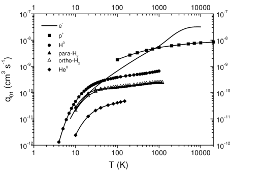
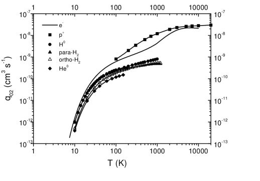
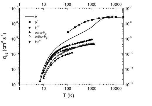
Figure 1: Excitation rates $q_{JJ^{\prime}}=q({{}^{3}P^{e}_{J}}\rightarrow{{}^{3}P^{e}_{J^{\prime}}})$ of the C⁰ fine-structure levels by collisions with various particles. The points - taken from the literature cited in the text - are interpolated by cubic splines.

We have also considered the effect of excitation of the upper ${}^{1}\mathrm{D}^{e}_{2}$ and ${}^{1}\mathrm{S}^{e}_{0}$ levels by collisions with electrons. We took the analytic fits to the Maxwellian-averaged collision strengths $\gamma$ for transitions involving these levels given by Péquignot & Aldrovandi [Péquignot & Aldrovandi 1976], and transformed them from LS coupling to the fine-structure levels according to their statistical weights:

$$\gamma\left({{}^{3}\mathrm{P}^{e}_{J}}\rightarrow{{}^{1}\mathrm{D}^{e}_{2}}\right) = \frac{2J+1}{9}\gamma\left({{}^{3}\mathrm{P}^{e}}\rightarrow{{}^{1}\mathrm{D}^{e}}\right)$$ (7)

$$\gamma\left({{}^{3}\mathrm{P}^{e}_{J}}\rightarrow{{}^{1}\mathrm{S}^{e}_{0}}\right) = \frac{2J+1}{9}\gamma\left({{}^{3}\mathrm{P}^{e}}\rightarrow{{}^{1}\mathrm{S}^{e}}\right)\ .$$

However, the inclusion of these levels can hardly influence the population of the ${}^{3}\mathrm{P}^{e}$ fine-structure levels at temperatures prevailing in ionization regions where the atom C⁰ is likely to be found. For example, even for temperatures as high as $T=10^{4}\ K$ the population ratio of the ${}^{3}\mathrm{P}^{e}_{1}$ level relatively to the ground state will increase by no more than 5 percent (10 percent for the ${}^{3}\mathrm{P}^{e}_{2}$ level). The test calculations were done taking into account only collisions by electrons (and spontaneous decays); if this is not the main excitation mechanism, then the error will be significantly smaller.

Excitation of the fine-structure levels by fluorescence was also investigated. We consider 108 allowed UV transitions involving the ground ${}^{3}\mathrm{P}^{e}$ levels and upper levels listed in the compilation of Verner, Verner & Ferland [Verner, Verner & Ferland 1996], which is based on Opacity Project calculations. If we adopt the radiation field of the Galaxy [Gondhalekar, Phillips & Wilson 1980], then the corresponding indirect excitation rates will be $\Gamma_{01}=3.5\ 10^{-10}\ \mathrm{s}^{-1}$ and $\Gamma_{02}=2.8\ 10^{-10}\ \mathrm{s}^{-1}$.

In fig. 2 we have plotted the population ratios of the C⁰ fine-structure levels taking into account collisions by hydrogen atoms (the main collision partner in ionization regions where the atom C⁰ is found), the CMBR and fluorescence induced by the radiation field of the Galaxy.

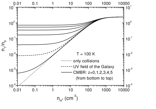
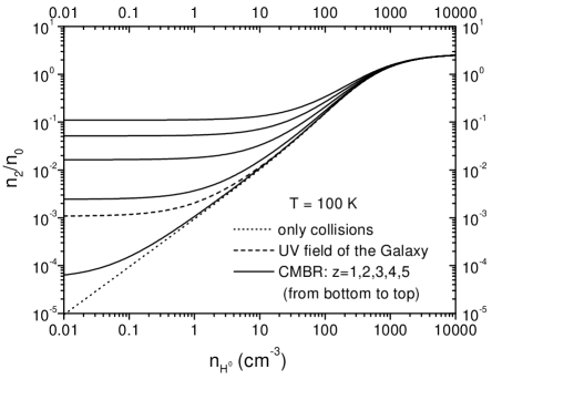
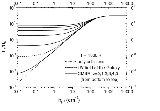
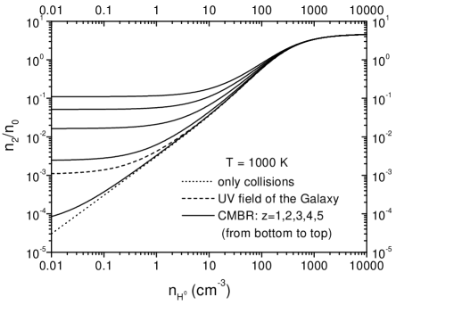
Figure 2: Population ratios of the C⁰ fine-structure levels relatively to the ground state $n_{J}/n_{0}=n({{}^{3}\mathrm{P}^{e}_{J}})/n({{}^{3}\mathrm{P}^{e}_{0}})$ calculated under various physical conditions. The curve for the $n_{2}/n_{0}$ population ratio for $z=0$ coincides with the curve taking only collisions into account.

We compared our results with the previous calculations by Keenan [Keenan 1989]. He considered the effect of collisions by electrons and hydrogend atoms, as well as fluorescence induced by the radiation field of the Galaxy. Test calculations revealed good overall agreement with the values obtained by Keenan, with differences typically less than 15 percent.

2.3 The ion C⁺

The ground state of the C⁺ ion consists of the 2s²2p ${}^{2}\mathrm{P}^{o}_{\frac{1}{2},\frac{3}{2}}$ doublet levels. The energy of the fine-structure excited level relatively to the ground state is 63.42 cm^-1, and the transition probability is $A_{\frac{3}{2}\frac{1}{2}}=2.291\ 10^{-6}\ \mathrm{s}^{-1}$.

Our model ion includes the five lowest LS terms: 2s²2p ${}^{2}\mathrm{P}^{o}$ and the 2s 2p² configurations ${}^{4}\mathrm{P}^{e}$, ${}^{2}\mathrm{D}^{e}$, ${}^{2}\mathrm{S}^{e}$ and ${}^{2}\mathrm{P}^{e}$, making a total of ten levels when the fine-structure splitting is accounted for. The energies were taken from Moore [Moore 1970] and the transition probabilities from the Iron Project calculation of Galavís, Mendoza & Zeippen [Galavís, Mendoza & Zeippen 1998].

As the fine-structure levels of C⁺ are more separated than the C⁰ levels, the CMBR will play a significant role at higher redshifts only, as one can see from the excitation rates given in table 1 .

We take into account collisional excitation of the fine-structure levels with several particles. For the Maxwellian-averaged collision strengths for collisions by electrons we have adopted the calculation of Blum & Pradhan [Blum & Pradhan 1992]. As their results differ by only 2 percent from the earlier calculation of Keenan et al. [Keenan et al. 1986], we have also included the later’s results at temperature values not covered by Blum & Pradhan’s calculation as a means of broadening the available temperature range. We took excitation rates by collisions with hydrogen atoms from Launay & Roueff [Launay & Roueff 1977b], extrapolated to $T>1000$ K by Keenan et al. [Keenan et al. 1986]. Other collision particles taken into account are protons [Foster, Keenan & Reid 1997] and molecular hydrogen [Flower & Launay 1977]. Fig. 3 compares the excitation rates with the various particles.

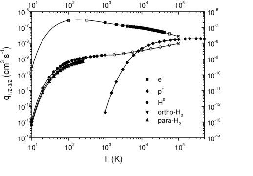
Figure 3: Excitation rates $q_{\frac{1}{2}\frac{3}{2}}=q({{}^{2}P^{o}_{\frac{1}{2}}}\rightarrow{{}^{2}P^{o}_{\frac{3}{2}}})$ of the C⁺ fine-structure level by collisions with various particles. The points - taken from the literature cited in the text - are interpolated by cubic splines.

We have complemented the work of Galavís et al. with the allowed transitions listed in the compilation of Verner et al., making a total of 48 transitions involving the ground ²P^o levels and upper levels. The indirect excitation rate by the UV radiation field of the Galaxy could then be determined: $\Gamma_{\frac{1}{2}\frac{3}{2}}=9.3\ 10^{-11}\ \mathrm{s}^{-1}$.

In order to assess the relevance of the 2s 2p² configuration upper levels in the relative population of the ground ${}^{2}\mathrm{P}^{o}_{\frac{1}{2},\frac{3}{2}}$ levels, we have performed test calculations comparing our 10-level model ion with the 2-level ion. At high temperatures the 2s 2p² configuration levels may be excited by collisions with hot electrons in the medium. However, the testcases have shown that this effect does not contribute significantly to the excitation of the ${}^{2}\mathrm{P}^{o}$ levels for temperatures $T\leq 30000$ K, where the discrepancies reach about 5 percent.

Therefore, for temperatures lower than 30000 K, only two levels can be taken into account. The population ratio of the excited fine-structure level relatively to the ground level is then expressed by:

$$\frac{n_{\frac{3}{2}}}{n_{\frac{1}{2}}}=\frac{Q_{\frac{1}{2}\frac{3}{2}}}{Q_{\frac{3}{2}\frac{1}{2}}} = \frac{K_{\frac{1}{2}\frac{3}{2}}+\Gamma_{\frac{1}{2}\frac{3}{2}}+\sum_{k}n^{k}q^{k}_{\frac{1}{2}\frac{3}{2}}}{A_{\frac{3}{2}\frac{1}{2}}+K_{\frac{3}{2}\frac{1}{2}}+\Gamma_{\frac{3}{2}\frac{1}{2}}+\sum_{k}n^{k}q^{k}_{\frac{3}{2}\frac{1}{2}}}$$

$$\cong \frac{K_{\frac{1}{2}\frac{3}{2}}+\Gamma_{\frac{1}{2}\frac{3}{2}}+\sum_{k}n^{k}q^{k}_{\frac{1}{2}\frac{3}{2}}}{A_{\frac{3}{2}\frac{1}{2}}+\sum_{k}n^{k}q^{k}_{\frac{3}{2}\frac{1}{2}}}\ .$$

The collisional de-excitation rates may be computed from the principle of detailed balance:

$$q_{\frac{3}{2}\frac{1}{2}}=\frac{1}{2}q_{\frac{1}{2}\frac{3}{2}}\mathrm{e}^{\frac{91.25}{T}}\ ,$$ (9)

with $T$ expressed in K.

In fig. 4 we have plotted the population ratio of the C⁺ excited fine-structure level relatively to the ground state under various physical conditions. As the ion C⁺ may coexist in both H i and H ii regions, we sample two cases of interest: a neutral medium at $T=1000$ K, and an ionized medium at $T=10000$ K. In the later case, in addition to collisions by electrons, we also consider proton collisions and set $n_{p}=n_{e}$. However, at $T=10000$ K their effect on the relative population ratio is only marginal (at the 5 percent level).

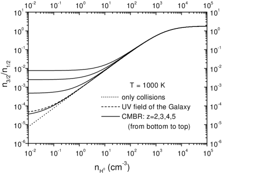
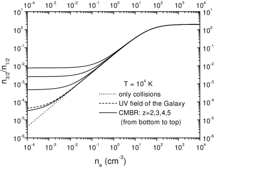
Figure 4: Population ratio of the C⁺ fine-structure level relatively to the ground state $n_{\frac{3}{2}}/n_{\frac{1}{2}}=n({{}^{2}\mathrm{P}^{o}_{\frac{3}{2}}})/n({{}^{2}\mathrm{P}^{o}_{\frac{1}{2}}})$ calculated under various physical conditions. The curves for $z\leq 1$ coincide with the curve taking only collisions into account. In the lower plot we have also taken proton collisions into account, $n_{p}=n_{e}$.

Previous work on the population of the C⁺ fine-structure levels taking into account fluorescence and collisions by electrons and hydrogen atoms was accoplished by Keenan et al. [Keenan et al. 1986]. Test calculations showed that our results seem to be in good agreement with their values, although it is not possible to make an accurate statement of the discrepancies, since they have published their results only in graphical form.

2.4 The atom O⁰

The ground state of the O⁰ atom is comprised of the 2s²2p⁴ ${}^{3}\mathrm{P}^{e}_{2,1,0}$ triplet levels. The energies of the fine-structure excited levels relatively to the ground state are 158.265 cm^-1 and 226.977 cm^-1. The transition probabilities are $A_{12}=8.865\ 10^{-5}\ \mathrm{s}^{-1}$, $A_{02}=1.275\ 10^{-10}\ \mathrm{s}^{-1}$ and $A_{01}=1.772\ 10^{-5}\ \mathrm{s}^{-1}$.

Our model atom includes the five lowest energy levels: 2s²2p⁴ ${}^{3}\mathrm{P}^{e}_{2,1,0}$, 2s²2p⁴ ${}^{1}\mathrm{D}^{e}_{2}$ and 2s²2p⁴ ${}^{1}\mathrm{S}^{e}_{0}$. The energies were taken from Moore [Moore 1993] and the transition probabilities from the Iron Project calculation of Galavís, Mendoza and Zeippen [Galavís, Mendoza & Zeippen 1997].

As the fine-structure levels of atomic oxygen are much more separated compared to atomic and singly ionized carbon, the CMBR will not play a major role as one can see from the excitation rates for the first excited level given in table 1 (the excitation rates for the second excited level are even lower).

The excited levels may be populated by collisions with particles present in the medium. Fig. 5 shows the collision rates for the fine-structure transitions induced by collisions with various particles. The rates for collisional excitation by electrons were taken from Bell, Berrington & Thomas [Bell, Berrington & Thomas 1998], by neutral hydrogen from Launay & Roueff [Launay & Roueff 1977a] and by neutral helium from Monteiro & Flower [Monteiro & Flower 1987]. For collisions with protons we have employed the analytic fits given by Péquignot [Péquignot 1990, Péquignot 1996].

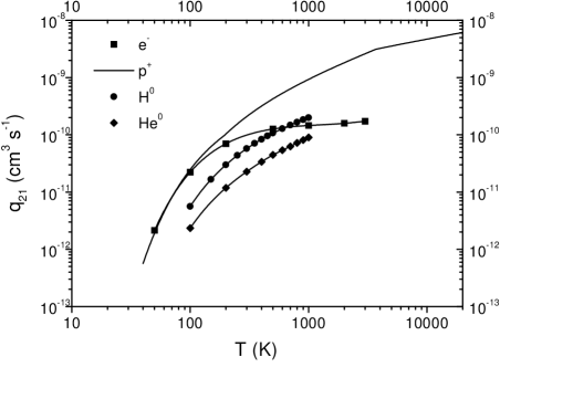
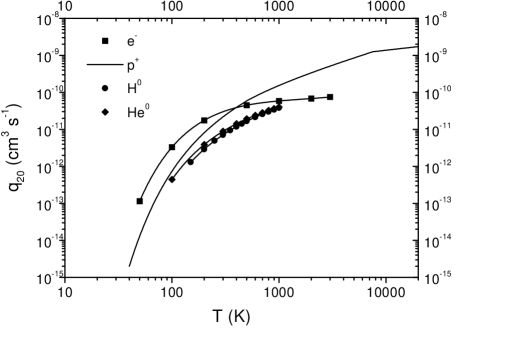
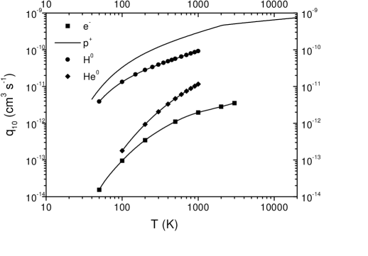
Figure 5: Excitation rates $q_{JJ^{\prime}}=q({{}^{3}P^{e}_{J}}\rightarrow{{}^{3}P^{e}_{J^{\prime}}})$ of the O⁰ fine-structure levels by collisions with various particles. The points - taken from the literature cited in the text - are interpolated by cubic splines.

For the sake of completeness, we have also considered collisional excitation of the upper ${}^{1}\mathrm{D}^{e}_{2}$ and ${}^{1}\mathrm{S}^{e}_{0}$ levels. We have taken the Maxwellian-averaged collision strengths for transitions induced by electrons involving these levels from Berrington & Burke [Berrington & Burke 1981]. The rate for the ${}^{3}\mathrm{P}^{e}$-${}^{1}\mathrm{D}^{e}$ transition induced by neutral hydrogen was taken from Federman & Shipsey [Federman & Shipsey 1983]. The rates were transformed from LS coupling to the individual fine-structure levels according to eq. (7).

After including 135 UV allowed transitions involving the ground ${}^{3}\mathrm{P}^{e}$ levels and upper levels from the work of Verner et al., we obtained the indirect excitation rates by the radiation field of the Galaxy: $\Gamma_{21}=3.9\ 10^{-11}\ \mathrm{s}^{-1}$ and $\Gamma_{20}=1.1\ 10^{-11}\ \mathrm{s}^{-1}$.

The relative populations of the ground ${}^{3}\mathrm{P}^{e}_{J}$ levels may be significantly affected by charge exchange reactions with hydrogen [Péquignot 1990, Péquignot 1996]:

$$\mathrm{H}^{+}+\,\mathrm{O}^{0}({{}^{3}\mathrm{P}^{e}_{J}})\rightarrow\mathrm{H}^{0}({{}^{2}\mathrm{S}^{e}_{1/2}})+\,\mathrm{O}^{+}({{}^{4}\mathrm{S}^{o}_{3/2}})$$ (10)

$$\mathrm{H}^{0}({{}^{2}\mathrm{S}^{e}_{1/2}})+\,\mathrm{O}^{+}({{}^{4}\mathrm{S}^{o}_{3/2}})\rightarrow\mathrm{H}^{+}+\,\mathrm{O}^{0}({{}^{3}\mathrm{P}^{e}_{J^{\prime}}})\,.$$

Consideration of this process would require a knowledge of the ionization state of cloud, which lies beyond the scope of this paper. Therefore, in our analysis we consider only the case of a primarily neutral medium.

In fig. 6 we plot the population ratios of the ground O⁰ fine-structure levels under various physical conditions. We consider collisions by hydrogen and helium atoms, assuming a helium abundance relative to hydrogen of 10 percent (by number). Collisions by helium atoms increases $n({{}^{3}\mathrm{P}^{e}_{1}})/n({{}^{3}\mathrm{P}^{e}_{2}})$ by only 5 percent and $n({{}^{3}\mathrm{P}^{e}_{0}})/n({{}^{3}\mathrm{P}^{e}_{2}})$ by 10 percent (reducing to zero close to LTE in the high density limit). The curves for $n({{}^{3}\mathrm{P}^{e}_{1}})/n({{}^{3}\mathrm{P}^{e}_{2}})$ corresponding to the inclusion of the effects of the CMBR at $z=5$ and the UV field of the Galaxy are coincident because the relevant excitation rates are of the same order $K^{z=5}_{21}\cong\Gamma^{\mathrm{G}}_{21}$.

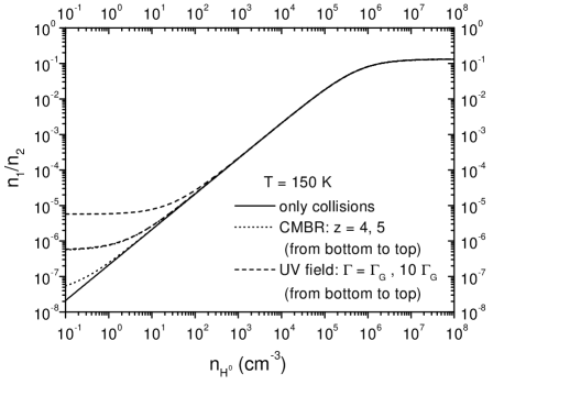
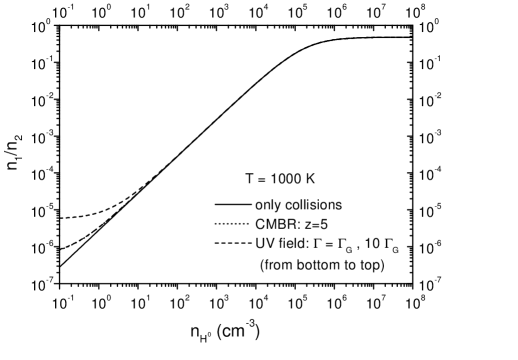
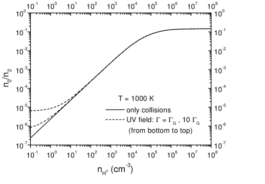
Figure 6: Population ratios of the O⁰ fine-structure levels relatively to the ground state $n_{J}/n_{2}=n({{}^{3}\mathrm{P}^{e}_{J}})/n({{}^{3}\mathrm{P}^{e}_{2}})$ calculated under various physical conditions.

Our results are not directly comparable to the work of Péquignot [Péquignot 1990, Péquignot 1996], who made assumptions on the ionization state of the gas. We point out, however, the importance of updating the electron excitation rates employed in their work - taken from Berrington [Berrington 1988] - to the more recent calculations of Bell et al., since the later’s results are substantially lower.

2.5 The ion Si⁺

The ground state of the Si⁺ ion consists of the 3s²3p ${}^{2}\mathrm{P}^{o}_{\frac{1}{2},\frac{3}{2}}$ doublet levels. The energy of the fine-structure excited level relatively to the ground state is 287.24 cm^-1, and the transition probability is $A_{\frac{3}{2}\frac{1}{2}}=2.17\ 10^{-4}\ \mathrm{s}^{-1}$.

Our model ion includes the three lowest LS terms: 3s²3p ${}^{2}\mathrm{P}^{o}$, 3s 3p² ${}^{4}\mathrm{P}^{e}$ and 3s 3p² ${}^{2}\mathrm{D}^{e}$, making a total of 7 levels when the fine-structure is accounted for. The energies were taken from Martin and Zalubas [Martin & Zalubas 1983]. The transition probabilities for the ${}^{2}\mathrm{P}^{o}_{\frac{3}{2}}\rightarrow{{}^{2}\mathrm{P}^{o}_{\frac{1}{2}}}$ forbidden transition was taken from Nussbaumer [Nussbaumer 1977], those for the ${}^{4}\mathrm{P}^{e}\rightarrow{{}^{2}\mathrm{P}^{o}}$ intercombination transitions from Calamai, Smith & Bergeson [Calamai, Smith & Bergeson 1993] and those for the ${}^{2}\mathrm{D}^{e}\rightarrow{{}^{2}\mathrm{P}^{o}}$ allowed transitions from Nahar [Nahar 1998].

Since the fine-structure levels of Si⁺ are too separated apart from eachother, the CMBR will not be an important excitation mechanism. Even for extremely high redshifts $z=5$, the excitation rate was found to be just $K_{\frac{1}{2}\frac{3}{2}}=4.7\ 10^{-15}\ \mathrm{s}^{-1}$.

Collisional processes considered are collisions by electrons [Dufton & Kingston 1991], protons [Bely & Faucher 1970] and hydrogen atoms [Roueff 1990]. In fig. 7 we have plotted the excitation rates by collisions with these particles.

Because the Maxwellian-averaged collision strength for the ${}^{2}\mathrm{P}^{o}_{\frac{1}{2}}-{{}^{2}\mathrm{P}^{o}_{\frac{3}{2}}}$ transition induced by electrons varies by no more than 6 percent in the calculated interval - $3.6\leq\log T\leq 4.6$ - we also indicate in fig. 7 what might be expected for the excitation rate down to $T=100$ K if we assume a constant value for the collision strength.

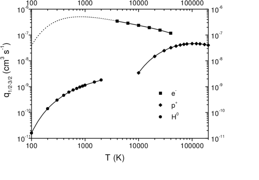
Figure 7: Excitation rates $q_{\frac{1}{2}\frac{3}{2}}=q({{}^{2}P^{o}_{\frac{1}{2}}}\rightarrow{{}^{2}P^{o}_{\frac{3}{2}}})$ of the Si⁺ fine-structure level by collisions with various particles. The points - taken from the literature cited in the text - are interpolated by cubic splines. The dotted line indicates an extrapolation of the excitation rate by electrons assuming a constant value for the corresponding Maxwellian-averaged collision strength.

In order to account for fluorescence, we consider 39 UV allowed transitions from the work of Nahar [Nahar 1998]. The indirect excitation rate by the UV field of the Galaxy was found to be $\Gamma_{\frac{1}{2}\frac{3}{2}}=1.1\ 10^{-9}\ \mathrm{s}^{-1}$.

At sufficiently high temperatures the ${}^{4}\mathrm{P}^{e}$ and ${}^{2}\mathrm{D}^{e}$ upper levels may be populated through collisions with hot electrons in the medium, and thereby influence the population of the ${}^{2}\mathrm{P}^{o}$ ground levels. To assess the relevance of this effect, we performed test calculations of the population ratios of the ${}^{2}\mathrm{P}^{o}$ fine-structure levels comparing the results obtained by the 2-level ion with those by the 7-level ion. Only collisions by electrons and spontaneous decays were considered. The test calculations revealed that the upper levels are not important for $T\leq 30000$ K, when the discrepancies reach about only 6 percent. Therefore, as for C⁺, for temperatures lower than this, only two levels can be taken into account. The system of statistical equilibrium equations (2) then yields:

$$\frac{n_{\frac{3}{2}}}{n_{\frac{1}{2}}}=\frac{Q_{\frac{1}{2}\frac{3}{2}}}{Q_{\frac{3}{2}\frac{1}{2}}}\cong\frac{\Gamma_{\frac{1}{2}\frac{3}{2}}+\sum_{k}n^{k}q^{k}_{\frac{1}{2}\frac{3}{2}}}{A_{\frac{3}{2}\frac{1}{2}}+\sum_{k}n^{k}q^{k}_{\frac{3}{2}\frac{1}{2}}}\ .$$ (11)

Excitation and de-excitation collisional rates are related by:

$$q_{\frac{3}{2}\frac{1}{2}}=\frac{1}{2}q_{\frac{1}{2}\frac{3}{2}}\mathrm{e}^{\frac{413.27}{T}}\ ,$$ (12)

with $T$ expressed in K.

In fig. 8 we plot the population ratios of the fine-strutucture levels of Si⁺ under various physical conditions. As Si⁺ may be the prevailing ionization state in both H i and H ii regions, we sample two cases of interest: a neutral medium at $T=1000$ K, and an ionized medium at $T=10000$ K.

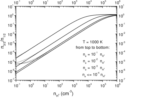
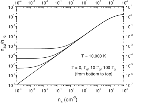
Figure 8: Population ratio of the Si⁺ fine-structure level relatively to the ground state $n_{\frac{3}{2}}/n_{\frac{1}{2}}=n({{}^{2}\mathrm{P}^{o}_{\frac{3}{2}}})/n({{}^{2}\mathrm{P}^{o}_{\frac{1}{2}}})$ calculated under various physical conditions. In the dotted curves in the upper plot we have also added the contribution of fluorescence induced by the UV field of the Galaxy.

Previous calculations of the population ratios of the ground fine-structure levels of Si⁺ were performed by Keenan et al. [Keenan et al. 1985]. Although test calculations under the same physical conditions considered by the authors appeared to reveal general agreement, it is difficult to quantify the discrepancies, since they published their results in graphical form only. We recommend the present calculations to the users, since they are based on more detailed and accurate atomic data.

2.6 The ion Fe⁺

The ground state of the Fe⁺ ion is comprised of the 3d⁶4s ${}^{6}\mathrm{D}^{e}_{\frac{9}{2},\frac{7}{2},\frac{5}{2},\frac{3}{2},\frac{1}{2}}$ sextet levels. Comparing to the other atoms/ions previously studied, the ion Fe⁺ has its fine-structure levels very separated apart from eachother and the transition probabilities are considerably higher. For example, the first excitated level is placed 384.790 cm^-1 above the ground level, and the corresponding transition probability is $A_{\frac{7}{2}\frac{9}{2}}=2.13\ 10^{-3}\ \mathrm{s}^{-1}$. Both factors will contribute to make the population ratios of the fine-structure levels of the Fe⁺ ion significantly low.

Our model ion includes the four lowest LS terms: 3d⁶4s ${}^{6}\mathrm{D}^{e}$, 3d⁷ ${}^{4}\mathrm{F}^{e}$, 3d⁶4s ${}^{4}\mathrm{D}^{e}$ and 3d⁷ ${}^{4}\mathrm{P}^{e}$, making a total of sixteen levels when the fine-structure splitting is accounted for. The energies were taken from Corliss & Sugar [Corliss & Sugar 1982] and the transition probabilities from the Iron Project calculation of Quinet, Le Dourneuf & Zeippen [Quinet, Le Dourneuf & Zeippen 1996] .

Due to the high separation of the fine-structure levels, the CMBR will not be an important excitation mechanism. For example, at $z=5$, the excitation rate to the first excited level is just $K_{\frac{9}{2}\frac{7}{2}}=3.5\ 10^{-18}\ \mathrm{s}^{-1}$.

The only collisional process for which we could find detailed excitation rates calculated in the literature were collisions by electrons. Fig. 9 shows the excitation rates by collisions with electrons for the most important transitions within the ${}^{6}\mathrm{D}^{e}$ ground term. The corresponding Maxwellian-averaged collision strengths were taken from the Iron Project calculation of Zhang & Pradhan [Zhang & Pradhan 1995].

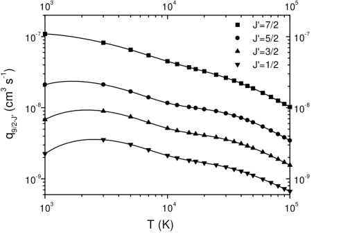
Figure 9: Excitation rates $q_{\frac{9}{2}J^{\prime}}=q({{}^{6}D^{e}_{\frac{9}{2}}}\rightarrow{{}^{6}D^{e}_{J^{\prime}}})$ of the Fe⁺ ground level to excited fine-structure levels by collisions with electrons. The corresponding Maxwellian-averaged collision strengths were taken from the Iron Project calculation of Zhang & Pradhan [Zhang & Pradhan 1995], and were interpolated by cubic splines.

Nussbaumer & Storey [Nussbaumer & Storey 1980] estimated the excitation rates by collisions with protons to be less than 10 percent of the corresponding excitation rates by collisions with electrons for temperatures as high as $T=15000$ K. However, as it is apparent from fig. 3 and fig. 7, the excitation rates for collisional processes involving positive ions and protons increase rapidly with temperature, so that one should be cautious when negleting collisions by protons at extremely high temperatures.

We also include 212 allowed transitions involving the ${}^{6}\mathrm{D}^{e}$ ground term levels and upper levels from the Iron Project calculation of Nahar [Nahar 1995]. The indirect excitation rates by fluorescence induced by the UV field of the Galaxy were found to be: $\Gamma_{\frac{9}{2}\frac{7}{2}}=7.0\ 10^{-10}\ \mathrm{s}^{-1}$, $\Gamma_{\frac{9}{2}\frac{5}{2}}=1.3\ 10^{-10}\ \mathrm{s}^{-1}$ and $\Gamma_{\frac{9}{2}\frac{3}{2}}=\Gamma_{\frac{9}{2}\frac{1}{2}}=0$ (the later rates are zero because those transitions are not eletric dipole allowed).

Previous calculations of the fine-structure population ratios of Fe⁺ levels were performed by Keenan et al. [Keenan et al. 1988]. They included only the two lowest LS states in their model ion, 3d⁶4s ${}^{6}\mathrm{D}^{e}$ and 3d⁷ ${}^{4}\mathrm{F}^{e}$, arguing that the next two LS states, 3d⁶4s ${}^{4}\mathrm{D}^{e}$ and 3d⁷ ${}^{4}\mathrm{P}^{e}$, do not affect significantly the population of the ${}^{6}\mathrm{D}^{e}$ ground levels. However, test calculations showed that considering the later LS terms increases the ${}^{6}\mathrm{D}^{e}$ ground level population ratios by as much as 17 percent for $T=10000$ K. The tests consisted of comparing the results of the 9-level and 16-level model ions taking only collisions by electrons (over various volume densities) and spontaneous decays into account. Therefore one should use the 16-level model ion for $T>10000$ K.

In order to assess the relevance at high temperatures of even higher-lying levels in the population ratios of the ${}^{6}\mathrm{D}^{e}$ ground levels, we have expanded our 16-level model ion to include the next two LS terms: 3d⁷ ${}^{2}\mathrm{G}^{e}$ and 3d⁷ ${}^{2}\mathrm{P}^{e}$, thereby increasing the total number of levels to 20.

Due to limitations of space, Quinet et al. list transition probabilities just for the strongest ($A_{ij}>10^{-3}\ \mathrm{s}^{-1}$) transitions involving these levels. Hence, for the sake of completeness, we decided to complement their work with the weaker transitions from Garstang [Garstang 1962]. The Maxwellian-averaged collision strengths for these transitions were taken from the Iron Project calculation of Bautista & Pradhan [Bautista & Pradhan 1996].

Test calculations with the 20-level model ion revealed that the last two LS terms do not affect at all the population ratios of the ${}^{6}\mathrm{D}^{e}$ ground levels up to $T\cong 20000$ K (the highest temperature considered in Bautista & Pradhan’s calculation).

Fig. 10 shows the population ratios of the Fe⁺ fine-structure levels as a function of electronic density for $T=10000$ K. We may note a slight inversion in the population of levels ${{}^{6}\mathrm{D}^{e}_{\frac{3}{2}}}$ and ${{}^{6}\mathrm{D}^{e}_{\frac{1}{2}}}$ at lower densities.

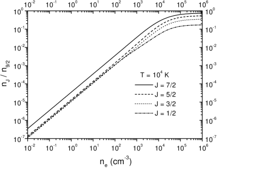
Figure 10: Population ratio of the Fe⁺ fine-structure levels relatively to the ground state $n_{J}/n_{\frac{9}{2}}=n({{}^{6}\mathrm{D}^{e}_{J}})/n({{}^{6}\mathrm{D}^{e}_{\frac{9}{2}}})$ as a function of electronic density.

Comparison of our results with those from the previous calculation of Keenan et al. under the same physical conditions revealed that our values for the population ratios of the fine-structure ground levels are a factor of 2-4 larger. We believe this can be traced back to the Maxwellian-averaged collision strengths employed, since the values from Zhang & Pradhan are much higher than those obtained by Berrington et al. [Berrington et al. 1988], quoted by Keenan et al. Since the Iron Project calculation of Zhang & Pradhan delineates the resonance structure of the collision strengths in more detail, the results obtained in the calculation presented here should be more reliable.

3 Physical Conditions

We now proceed to use our calculated atomic level population ratios to study the physical conditions in QSO absorbers.

Table 2 shows our sample of absorption line systems for which there are column density ratios of fine-structure lines reported in the recent literature.

Table 2: Observational data on the column density ratios of fine-structure lines in QSO absorbers retrieved from the literature.

#	QSO	$z_{\mathrm{em}}$	$z_{\mathrm{abs}}$	$\log$ N(H i)	ion	$N^{*}/N$ a	$T_{\mathrm{exc}}$ a	$T_{\mathrm{cmbr}}$ b	reference
1	PKS 1756+23	1.721	1.6748	$>\,20.3$	C i	$<\,1.2\,10^{-1}$ c	$<\,7.4$	7.289	Roth & Bauer [Roth & Bauer 1999]
2a	Q1331+17	2.084 d	1.77638	21.2 d	C i	$(3.1\,\pm\,0.3)\,10^{-1}$	$10.4\,\pm\,0.5$	7.566	Songaila et al. [Songaila et al. 1994b]
2b	Q1331+17	2.084 d	1.77654	21.2 d	C i	$(1.3\,\pm\,0.4)\,10^{-1}$	$7.4\,\pm\,0.8$	7.566	Songaila et al. [Songaila et al. 1994b]
3	Q0013-00	2.0835 e	1.9731	20.7 e	C i	$(4.0\,\pm\,0.8)\,10^{-1}$	$11.7\,\pm\,1.1$	8.102	Ge, Bechtold & Black [Ge et al. 1997]
3	Q0013-00	2.0835 e	1.9731	20.7 e	C ii	$(7.0\,\pm\,3.2)\,10^{-3}$	$16.2\,\pm\,1.3$	8.102	Ge, Bechtold & Black [Ge et al. 1997]
4	Q0149+33	2.43	2.140	20.5 f	C ii	$<\,9.6\,10^{-3}$	$<\,17.1$	8.557	Prochaska & Wolfe [Prochaska & Wolfe 1999]
5	Q1946+76	2.994	2.8443	20.27	C ii	$<\,2.1\,10^{-2}$	$<\,20.0$	10.476	Lu et al. [Lu et al. 1996b]
6	Q0636+68	3.174 g	2.9034	17.7 h	C ii	$<\,6.7\,10^{-3}$ i	$<\,16.0$	10.637	Songaila et al. [Songaila et al. 1994a]
7	Q0347-38	3.23	3.025	20.7 d	C ii	$<\,2.8\,10^{-2}$	$<\,21.4$	10.968	Prochaska & Wolfe [Prochaska & Wolfe 1999]
8	Q2212-16	3.992	3.6617	20.2	C ii	$<\,2.3\,10^{-2}$	$<\,20.5$	12.703	Lu et al. [Lu et al. 1996b]
9	Q2237-06	4.559	4.0803	20.5	C ii	$<\,4.4\,10^{-3}$	$<\,14.9$	13.844	Lu et al. [Lu et al. 1996b]
10	BRI 1202-07	4.7	4.3829	20.6	C ii	$<\,1.2\,10^{-2}$	$<\,18.0$	14.668	Lu et al. [Lu et al. 1996a]

^a Errors are $1\sigma$ CL, while upper limits are $2\sigma$ CL.

^b Assuming the temperature-redshift relation predicted by the standard model.

^c $2\sigma$ upper limit on $N^{*}$ obtained by private communication with the author.

^d Pettini et al. [Pettini et al. 1994].

^e Ge & Bechtold [Ge & Bechtold 1997].

^f Wolfe et al. [Wolfe et al. 1993].

^g Sargent, Steidel & Boksenberg [Sargent et al. 1989].

^h Derived from the optical depth of the LL discontinuity: $\tau_{\mathrm{LL}}=3.5$ [Sargent et al. 1989].

ⁱ Given the strong saturation of the ground fine-structure line, we adopt $N>1.5\,10^{14}\,\mathrm{cm}^{-2}$ instead of the profile fitting value $N=4.6\,10^{14}\,\mathrm{cm}^{-2}$ preferred by Songaila et al. [Songaila et al. 1994a].

The sample includes DLA systems ($\log\mathrm{N}(\hbox{H\,{\sc i}})>20.3$), and only one LL system at $z_{\mathrm{abs}}=2.9034$.

We have not included any associated system, since their close proximity to the QSO could make them susceptible to the influence of the background radiation source, therefore requiring a case by case analysis that lies beyond the scope of this paper. The fine-structure lines are, however, a valuable tool to infer the physical conditions in such systems. In particular, the knowledge of the ionization state of the systems coupled with the information on the volumentric density afforded by the fine-structure lines allows one to place limits on the distance between the absorber and the QSO, giving a clue to infer whether they correspond to intervening clouds or to material ejected from the QSO [Turnshek, Weymann & Williams 1979, Morris et al. 1986, Tripp, Lu & Savage 1996, Srianand & Petitjean 2000].

So far, all the fine-structure lines observed belong to either C⁰ or C⁺. Owing to its low ionization fraction (since its ionization potential is lower than that of hydrogen), atomic carbon is very seldom detected. The three systems listed in table 2 correspond to all of the presently known C i systems, apart from the system observed towards the BL Lac object 0215+015 [Blades et al. 1982, Blades et al. 1985].

As we gathered observational data from the literature, we rejected any line falling within the Ly-$\alpha$ forest region of the spectrum. Prochaska [Prochaska 1999] observed the C ii^∗ 1335 fine-structure transition in a LL system at $z_{\mathrm{abs}}=2.652$ towards Q2231-00. However, since this transition falls within the Ly-$\alpha$ forest in this object and therefore may have been subject to significant contamination, his claimed value on the column density N(C ii^∗) should be regarded at most as an upper limit to the true value. For the same reason we disregarded the DLA system at $z_{\mathrm{abs}}=3.054$ towards Q0000-26 observed by Giardino & Favata [Giardino & Favata 2000]. Although the authors quoted their value for N(C ii^∗) as an upper limit, we argue that in principle significant contamination could also be taking place on the ground fine-structure line, thereby also affecting N(C ii) and driving the ratio $N^{*}/N$ in the opposite sense.

Unfortunately, the ground C ii 1334 line is often heavily saturated; to circunvent this problem there have been many alternative approaches to derive the N(C ii) column density by other indirect methods. Prochaska [Prochaska 1999] used the ratio of N(C ii)/N(Fe ii) in a velocity region where the ground C ii line was not saturated to derive the corresponding value at the component where the C ii^∗ line was detected. Outram, Chaffee & Carswell [Outram, Chaffee & Carswell 1999] assumed a carbon abundance relative to iron [C/Fe]$>$-0.3 to obtain a tighter lower limit on the N(C ii) column density in a DLA system at $z_{\mathrm{abs}}=2.62$ towards GB1759+75. In our sample we have included only direct measurements on the column densities.

In sections 3.1-3.2 below, we will separately study the DLA and LL systems in our sample. Again, as a working hypothesis we shall assume the temperature-redshift relation as predicted by the standard model. The validity of this relation is discussed in section 3.3.

3.1 DLA systems

DLA systems have very high neutral hydrogen column densities ($\log\mathrm{N}(\hbox{H\,{\sc i}})>20.3$). This makes them effectively shielded from the ionizing radiation, causing their contents to be essentially neutral material [Viegas 1995].

We use the fine-structure lines column density ratios observed in the DLA systems listed in table 2 to set upper limits to their neutral hydrogen volume densities $n_{\mathrm{H}^{0}}$ and to the intensities of the UV radiation field present. Given the high neutral hydrogen column density, probably all of the hydrogen ionizing radiation will be absorbed, leaving very few photons with energies greater than 1 Ryd. The spectral shape of the UV radiation field will then be similar to the one found in our own galaxy, and we therefore assume the UV radiation field of Gondhalekar et al. multiplied by a constant factor $f_{\mathrm{G}}$.

Table 3 shows the upper limits to $n_{\mathrm{H}^{0}}$ and $f_{\mathrm{G}}$ for the DLA systems in our sample. They represent firm upper limits to the true values, because the single excitation mechanism considered to obtain the upper limit - i.e., collisions by neutral hydrogen atoms to obtain $n_{\mathrm{H}^{0}}$ and fluorescence to obtain $f_{\mathrm{G}}$ - may not be the dominating one and also because for most systems the population ratios were just upper limits.

Table 3: Physical conditions in DLA systems. The quoted values for $f_{\mathrm{G}}$ and $n_{\mathrm{H}^{0}}$ are upper limits, whereas those for $l$ and $M$ are lower limits. The CL is $2\sigma$. The second figure next to each entry corresponds to the inclusion of the CMBR (if only one value appears, it is not altered to the last digit displayed).

		$T=100$ K			$T=1000$ K
#	$f_{\mathrm{G}}$	$n_{\mathrm{H}^{0}}$ [cm-3]	$l$ [pc]	$M$ [$M_{\sun}$]	$n_{\mathrm{H}^{0}}$ [cm-3]	$l$ [pc]	$M$ [$M_{\sun}$]
1	16 / 0.79	16 / 0.79	4.0 / 81	26 / 10600	6.9 / 0.34	9.4 / 192	142 / 58800
2a	42 / 25	43 / 26	11 / 19	1540 / 4290	18 / 11	27 / 46	8910 / 24900
2b	16 / -	16 / -	30 / -	10700 / -	6.9 / -	70 / -	59600 / -
4	236 / 235	35 / 34	2.8	19	12	7.8	146 / 148
5	518 / 510	77 / 75	0.79 / 0.80	0.93 / 0.96	27	2.2	7.3 / 7.5
7	703 / 691	105 / 103	1.6	10	37 / 36	4.4	77 / 79
8	582 / 544	86 / 81	0.60 / 0.64	0.45 / 0.52	31 / 29	1.7 / 1.8	3.6 / 4.1
9	107 / 39	16 / 5.7	6.2 / 17	93 / 692	5.7 / 2.1	17 / 47	711 / 5320
10	307 / 209	45 / 31	2.9 / 4.2	26 / 57	16 / 11	8.0 / 12	205 / 445

Because the collisional excitation rate is temperature dependent, so will be the derived upper limits on $n_{\mathrm{H}^{0}}$; we assume two values of kinetic temperature characteristic of H i regions: $T=100$ K and $T=1000$ K.

If excitation by the CMBR is taken into account the upper limits become tighter (lower), as indicated by the second figure next to each entry in table 3 (if only one value appears, it remains unchanged to the last significant digit displayed). Accounting for the CMBR affects considerably the results for the C i systems (objects 1 and 2), since it is an important excitation mechanism for C⁰ as mentioned earlier in section 2.2. Note the striking difference between both values for object 1, which has an excitation temperature very close to the predicted CMBR temperature. We can not consider the CMBR for object 2b, since the excitation temperature is slightly lower than the CMBR temperature. As for the remaining C ii systems the result is changed significantly only for the $z>4$ regions (objects 9 and 10), when the CMBR starts to play a significant role at the neutral hydrogen densities involved (cf. fig. 4, top).

Collisions with molecular hydrogen are not likely to be relevant in our analysis, since the molecular fraction usually seen in DLA systems is exceedingly small: $f(\mathrm{H}_{2})\equiv 2N(\mathrm{H}_{2})/N(\mathrm{H})<2\,10^{-4}$, reaching as low as $f(\mathrm{H}_{2})=4\,10^{-8}$ in the $z_{\mathrm{abs}}=3.3901$ DLA system towards Q0000-26 [Levshakov et al. 2000]. Two exceptions are object 3 in our sample [Ge & Bechtold 1997] and the $z_{\mathrm{abs}}=2.34$ DLA system towards Q1232+08 [Ge, Bechtold & Kulkarni 2000], with $f(\mathrm{H}_{2})=0.22$ and 0.07, respectively. In any case that would imply $n_{\mathrm{H}_{2}}q^{\mathrm{H}_{2}}_{ij}<<n_{\mathrm{H}^{0}}q^{\mathrm{H}^{0}}_{ij}$, as typically $q^{\mathrm{H}_{2}}_{ij}<q^{\mathrm{H}^{0}}_{ij}$ (cf. figs. 1 and 3).

From table 3 we see that the ratio of fine-structure lines observed in DLA systems constrain their neutral hydrogen densities to be lower than tens of cm^-3 (or a few cm^-3 in the best cases), and the UV radiation field to be lower than two orders of magnitude the radiation field present in our galaxy (or one order of magnitude in the best cases).

Naturally, we could also have placed upper limits to the electron density $n_{e}$. The upper limits on $n_{e}$ derived from C ii lines would be about two orders of magnitude lower than the corresponding upper limits on $n_{\mathrm{H}^{0}}$ listed in table 3, i.e., in the approximate inverse ratio of the corresponding collision rates $q^{e}_{\frac{1}{2}\frac{3}{2}}/q^{\mathrm{H}^{0}}_{\frac{1}{2}\frac{3}{2}}\approx 10^{2}$ (fig. 3). For C⁰ this ratio is no more than 10 in the relevant temperature region (fig. 1). As DLA systems are comprised of mostly neutral material, the free electrons will come mainly from neutral atoms which have an ionization potential lower than that of hydrogen, such as C⁰, an whose (solar) elemental abundance relative to hydrogen is of order $10^{-4}$. Therefore, we would expect beforehand $n_{e}\approx 10^{-4}n_{\mathrm{H}^{0}}$, and the fine-structure lines would not provide a meaninful constraint on the electron density. The electron/neutral hydrogen density ratio may be even lower if we consider that DLA systems may exhibit abundances as low as two orders of magnitude below solar (e.g. Pettini et al. 1994).

We can also estimate the characteristic sizes and total masses of the absorbing clouds responsible for the DLA systems; these will be given by:

$$l = \frac{\mathrm{N}(\mathrm{H})}{n_{\mathrm{H}}}$$ (13)

$$M = m_{p}n_{\mathrm{H}}\,l^{3}=m_{p}\mathrm{N(H)}\,l^{2}\,,$$

where $m_{p}$ is the proton’s mass and N(H) and $n_{\mathrm{H}}$ are the total hydrogen column and volume densities, respectively.

For DLA systems we can make the replacement $\mathrm{N(H)}\cong\mathrm{N(H\,{\sc i})}$ and $n_{\mathrm{H}}\cong n_{\mathrm{H}^{0}}$ ; hence we can use our upper limits on $n_{\mathrm{H}^{0}}$ to set lower limits to the characteristic sizes and total masses of the intervening clouds. We see from table 3 that our constraints imply characteristic sizes larger than a few pc (tens of pc in the best cases) and lower limits for the total masses that vary from $10^{0}$ to $10^{5}$ solar masses.

In deriving the cloud sizes and masses above, we have implicitly assumed that most of the hydrogen column density is in the same component where the fine-structure lines could be measured. Altough it would be much more difficult to detect the excited fine-structure line in the velocity component with the lowest associated hydrogen column density, we can not rule out the possibility that this is compensated by a higher metalicity and intensity of local excitation mechanisms.

We now focus our attention to object 3 in our sample, which exhibits both C i and C ii fine-structure lines. In fig. 11 we derive the neutral hydrogen volume density as a function of the intensity of the UV radiation field based upon the column density ratios of C i and C ii lines (and for the two values of kinetic temperature considered before; the CMBR is included). If we assume that C⁰ and C⁺ are located within the same ionization region in the cloud, then the physical conditions will be described by the intersection of both curves. For $T=100$ K we have $n_{\mathrm{H}^{0}}=24$ cm^-3 and $f_{G}=11$, whereas for $T=1000$ K we have $n_{\mathrm{H}^{0}}=14$ cm^-3 and $f_{G}=8$. Therefore, regardless of the kinetic temperature adopted, the UV field present must be one order of magnitude more intense than in our galaxy. This contrasts with object 1, where the observed C i lines constrain the UV field to be lower than in our galaxy. In the detailed photoionization model constructed by Ge et al. the physical conditions prevailing in most regions of the cloud are: $T=100$ K, $n_{\mathrm{H}^{0}}=21.0\pm 9.6$ cm^-3, $f_{G}=17.0$ and $n_{e}=5.0\,10^{-4}n_{\mathrm{H}^{0}}$. Assuming their value for $n_{\mathrm{H}^{0}}$ we have $l=7.7\pm 3.6$ pc and $M=240\pm 160\,M_{\sun}$.

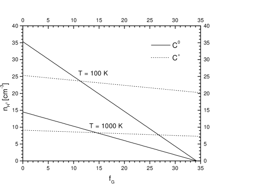
Figure 11: Physical conditions in object 3 in our sample (the CMBR is included).

3.2 LL systems

The LL systems differ considerably from the DLA systems studied before for beeing significantly ionized. The source of the ionizing radiation in these systems is usually assumed to be the UV extragalactic background, as the integrated radiation field of all QSOs attenuated by the intergalactic medium [Haardt & Madau 1996].

Some authors claim for a local origin to the source of ionization [Viegas & Friaça 1995]. In particular, the puzzling observations of column densities of C, N and O ions in various ionization states as well as of He i in LL systems towards Q1700+64 [Vogel & Reimers 1993, Reimers & Vogel 1993] cannot be simultaneously explained by photoionization models based on the UV background as the source of ionization. These systems are successfully interpreted by the hot halo model [Viegas & Friaça 1995]; in this model the LL systems are identified as cold condensations embedded in a hot halo formed during the early stages of galaxy evolution, which acts as the source of ionization.

Photoionization models typically constrain the ionization parameter $U\equiv\frac{\Phi_{\mathrm{H}}}{n_{\mathrm{H}}c}$ ($\Phi_{\mathrm{H}}$ is the total photon flux of hydrogen ionizing radiation); the fine-structure lines might be used to independently constrain the volumetric density and test the hypothesis of a given radiation field as beeing the source of ionization. If the density determined from the fine-structure lines, together with the ionization parameter determined from ionization models based on the UV background imply a higher intensity for the ionizing radiation field than expected, that would be a strong evidence for a local origin to the true ionization source.

For the only LL system in our sample (object 6 in table 2), we derive a $2\sigma$ upper limit to the electronic density of $n_{e}<0.15$ cm^-3, assuming a kinetic temperature $T=10^{4}$ K characteristic of photoionized regions. We have included the minor contribution from the CMBR and collisions by protons (assuming a fully ionized medium $n_{p}=n_{e}$), although they affect the result only at the 10 percent level. Fluorescence plays a negligible role. In table 4 we show the indirect excitation rates of C⁺ fine structure levels for the hot halo models considered by Viegas & Friaça; in any case we have $\Gamma_{\frac{1}{2}\frac{3}{2}}<<\,n_{e}q^{e}_{\frac{1}{2}\frac{3}{2}}$. The indirect excitation rate induced by the UV background turns out to be even lower; we have adopted the revised calculation of Madau, Haardt & Rees [Madau, Haardt & Rees 1999] to obtain an indirect excitation rate at the observed redshift of $\Gamma_{\frac{1}{2}\frac{3}{2}}=3.1\,10^{-12}$ s^-1.

Table 4: Indirect excitation rates of C⁺ fine-structure levels by the radiation fields predicted by hot halo models. Each model, taken from Viegas & Friaça, corresponds to a given age and distance from the center of the forming galaxy.

$t$ (Gyr)	$r$ (kpc)	$\Gamma_{\frac{1}{2}\frac{3}{2}}$ (s-1)
0.206	30	6.8 10-10
0.206	100	6.2 10-11
0.3644	30	1.3 10-11
0.3644	100	1.2 10-12

3.3 The CMBR temperature-redshift relation

The CMBR constitutes one of the cornerstones of the hot Big Bang model, which makes three basic quantitative predictions on its properties:

1. it is isotropic and homogeneous;

2. it has a black-body spectrum,

3. it cools as the universe expands according to the relation $T=T_{0}(1+z)$.

Over the past decade, the advent of the COBE satellite has allowed the confirmation of the isotropy [Smoot et al. 1992] and black-body spectral shape [Mather et al. 1994] to unprecedented precision, giving a present day temperature of $T_{0}=2.725\pm 0.001$ K ($1\sigma$ error) as determined from the FIRAS instrument [Mather et al. 1999, Smoot & Scott 2000].

Any direct means of measuring the CMBR temperature can just provide us with the value of its current temperature, forcing us to resort to other indirect methods to test the temperature-redshift relation predicted by the standard model. The best alternative is to use atomic and molecular transitions seen in the spectra of QSO absorbers [Meyer 1994]. It is worth noting that the observation of CN absorption lines from diffuse interstellar clouds towards bright stars in the Galaxy yielded $T_{0}=2.729^{+0.023}_{-0.031}$ K, in excellent agreement with the COBE FIRAS result [Roth 1992, Roth, Meyer & Hawkins 1993, Roth & Meyer 1995].

Unfortunately, molecular transitions are not commonly seen in the spectra of QSO absorbers. Apart from H₂, so far molecules have been identified in just four absorption systems [Wiklind & Combes 1994, Wiklind & Combes 1995, Wiklind & Combes 1996a, Wiklind & Combes 1996b]. Surprisingly, in one of them [Wiklind & Combes 1996b] the rotational transitions from several molecules indicated an excitation temperature $T_{\mathrm{exc}}=4\pm 2$ K ($3\sigma$ error), lower than the expected CMBR temperature $T=5.14$ K predicted at the observed redshift. The low excitation temperature in this object is, nevertheless, due to the effect of a microlensing event (Combes 2000, private comm.). Molecular absorption systems are often gravitational lenses, since the impact parameter to the foreground galaxy must be close to zero in order to allow the detection of molecules. Hence, we believe that atomic lines are better suited to study the temperature of the CMBR at high redshifts.

We can use the population ratios of the fine-structure levels for the absorption systems collected in table 2 to constrain the temperature of the CMBR at their redshifts. For each observed ion the excitation temperature will be given by

$$T_{\mathrm{exc}} = \frac{23.60}{\ln(3/(n^{*}/n))}\qquad\mathrm{for\,\,C}^{0}$$ (14)

$$T_{\mathrm{exc}} = \frac{91.25}{\ln(2/(n^{*}/n))}\qquad\mathrm{for\,\,C}^{+}\,,$$

with temperatures given in K.

The excitation temperatures so obtained represent firm upper limits to the temperature of the CMBR, because local excitation mechanisms may also contribute significantly to populate the excited levels. In fig. 12 we plot the excitation temperatures along with the expected temperature of the CMBR according to the standard model prediction. For most systems, either the signal to noise ratio of the spectrum was not high enough to detect the excited fine structure line, or the ground C ii line was strongly saturated. Therefore for these systems the excitation temperature itself is also an upper limit, and this is indicated in fig. 12 by a downward arrow. The point labelled ”molecules” corresponds to the puzzling observation of Wiklind & Combes [Wiklind & Combes 1996b] discussed above.

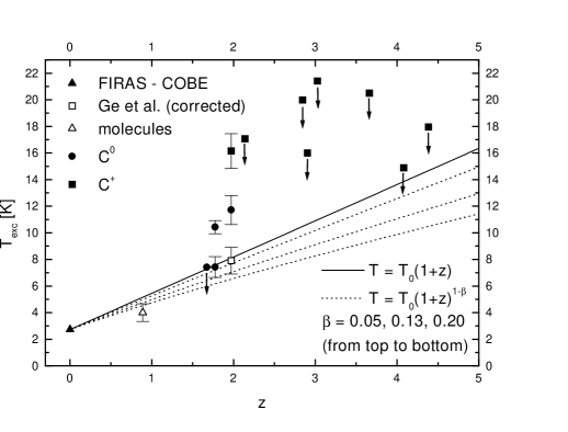
Figure 12: Excitation temperatures derived from fine-structure absorption lines. The solid line is the temperature of the CMBR according to the temperature-redshift relation given by the standard model, while alternative models with photon creation predict a lower temperature (dotted lines). Error bars are $1\sigma$ CL, whereas upper limits are $2\sigma$ CL.

Phillips [Phillips 1994] supports a closed steady-state model that predicts considerably lower temperatures to the CMBR compared to the standard model; e.g. for the $z=2.9$ C ii system observed by Songaila et al. [Songaila et al. 1994a]: $T_{\mathrm{obs}}=6.55$ K.

Alternative models in which photon creation takes place as the Universe expands predict a more general temperature-redshift relation [Lima, Silva & Viegas 2000]:

$$T=T_{0}(1+z)^{1-\beta}\,,$$ (15)

where $\beta$ is a parameter to be adjusted from the observations, within the range $0\leq\beta\leq 1$. Equation (15) therefore gives temperatures lower than predicted by the standard model (fig. 12).

It has been stated that any scenario that does not preserve the number of photons would introduce large distortions in the black-body spectrum of the CMBR [Steigman 1978]. However, it was shown that for the class of models that follow the temperature law (15) the Planckian spectral shape is not destroyed as the Universe evolves [Lima 1996, Lima 1997]. In these models the total entropy of Universe increases with time, but the entropy per particle remains constant.

Big Bang nucleosynthesis arguments, however, severely limit the value of the free parameter to $\beta<0.13$ [Birkel & Sarkar 1997].

Inspection of fig. 12 reveals that current measurements do not require any extra ingredients to the standard model, since the totality of the points lie above the linear temperature law. However, a conclusive statement could only be made after correcting for local excitation mechanisms, in order to convert the excitation temperature upper limits to the actual temperature of the CMBR. Altough some points in fig. 12 appear to be dangerously close to the standard model prediction, it could be that additional local excitation mechanisms are negligible compared to excitation by the CMBR in these systems. In that case, the excitation temperature would provide a direct measure of the CMBR temperature.

For object 3 in our sample, Ge et al. [Ge et al. 1997] constructed a detailed photoionization model to account for the local excitation mechanisms. They obtained $T=7.9\pm 1.0$ K, whereas the standard model prediction is $T=8.102\pm 0.003$ K (fig. 12).

If the temperature law given by the standard model turns out to be incorrect, it would pose a serious source of difficulty, since not even the presence of a cosmological constant would alter the predicted temperature-redshift relation [Lima, Silva & Viegas 2000]. On the other hand, if it is confirmed by the observations, that would add another success to its list of triumphs with a bonus: since each absorbing region is located at a different site of the Universe, we could also assess its homogeneity.

4 Conclusions

We have presented new theoretical calculations of population ratios of the ground fine-structure levels of C⁰, C⁺, O⁰, Si⁺ and Fe⁺. The literature was searched for the most recent and reliable atomic data available to date. Various possible excitation mechanisms are taken into account. We encourage the user to make use of the available Fortran code to obtain accurate predictions in his/her applications, rather then rely on approximate practical formulas that are valid only for a limited range of physical conditions.

We have retrieved from the literature observational data on the column density ratios derived from the fine-structure lines, and confronted them with our theoretical calculations to infer the physical conditions prevailing in DLA and LL systems. Currently only C i and C ii fine-structure lines have been observed; future detection of lines originating from less excited atoms/ions such as O⁰, Si⁺ and Fe⁺ (which also have resonant lines redward the Ly-$\alpha$ forest) might aid to better constrain the physical conditions.

For the DLA systems, the neutral hydrogen volumetric density is lower than tens of cm^-3 (a few cm^-3 in the best cases) and the UV radiation field is less intense than two orders of magnitude the UV field of the Galaxy (one order of magnitude in the best cases). Their characteristic sizes are higher than a few pc (tens of pc in the best cases) and lower limits for their total masses vary from $10^{0}$ to $10^{5}$ solar masses.

For the only LL system in our sample, we derived $n_{e}<0.15$ cm^-3. As more observations become available, it may be possible to use the information contained in the fine-structure lines to help determine the nature of the source of ionization of these systems.

The fine-structure lines in QSO absorbers also provide a method to test the temperature-redshift relation for the CMBR predicted by the standard model. Current observations do not contradict the linear temperature law, although a conclusive statement could only be made after accounting for local excitation mechanisms in order to correct the excitation temperatures to the actual temperature of the CMBR. That would require a knowledge of the ionization state of the cloud, after appropriate modeling by a photoionization code.

A substantial improvement from the theoretical standpoint could be achieved by analysing together the ionization state of the cloud and the excitation of the fine-structure levels, by coupling our code - popratio - to a larger photoionization code. Presently, all studies based on the excitation of the fine-structure levels were carried out separately from the photoionization modeling, considering average physical conditions throughout the entire cloud (e.g. Ge et al., Giardino & Favata).

By carrying out both analyses simultaneously, we could further refine our models and eliminate the need for all assumptions we have maden in our analyses of the fine-structure lines. The intensities of the excitation mechanisms could vary across the cloud, and it would no longer be necessary to stick to the simplistic case of a perfect homogeneous cloud, that we implicitly assumed when we wrote down eq. (1). Moreover, we could generalize our statistical equilibrium equations (2) to include terms which require the knowledge of the ionization state of the cloud, such as recombination and charge exchange. It would also be possible to account for optical depth effects, allowing us to drop the assumption that all transitions considered are optically thin.

On the observational side, there is also clearly a need for better measurements, since for the great majority of the systems only upper limits to the column density ratios are available. As the future generations of more powerful telescopes equipped with high resolution spectrographs continue to push the detection limits to even weaker lines, more information could be available by observing atoms/ions other than C⁰ and C⁺.

References

- [Bahcall & Wolf 1968] Bahcall J.N., Wolf R.A., 1968, ApJ, 152, 701
- [Bautista & Pradhan 1996] Bautista M.A., Pradhan A.K., 1996, A&AS, 115, 551
- [Bell, Berrington & Thomas 1998] Bell K.L., Berrington K.A., Thomas M.R.J., 1998, MNRAS, 293, L83
- [Bely & Faucher 1970] Bely O., Faucher P., 1970, A&A, 6, 88
- [Berrington 1988] Berrington K.A., 1988, J. Phys. B, 21, 1083
- [Berrington & Burke 1981] Berrington K.A., Burke P.G., 1981, Planet. Space Sci., 29, 377
- [Berrington et al. 1988] Berrington K.A., Burke P.G., Hibbert A., Mohan M., Baluja K.L., 1988, J. Phys. B, 21, 339
- [Birkel & Sarkar 1997] Birkel M., Sarkar S., 1997, Astrop. Phys., 6, 197
- [Blades et al. 1982] Blades J.C., Hunstead R.W., Murdoch H.S., Pettini M., 1982, MNRAS, 200, 1091
- [Blades et al. 1985] Blades J.C., Hunstead R.W., Murdoch H.S., Pettini M., 1985, ApJ, 288, 580
- [Blum & Pradhan 1992] Blum R.D., Pradhan A.K., 1992, ApJS, 80, 425
- [Calamai, Smith & Bergeson 1993] Calamai A.G., Smith P.L., Bergeson S.D., 1993, ApJ, 415, L59
- [Corliss & Sugar 1982] Corliss C., Sugar J., 1982, J. Phys. Chem. Ref. Data, 11, 135
- [Dufton & Kingston 1991] Dufton P.L., Kingston A.E., 1991, MNRAS, 248, 827
- [Federman & Shipsey 1983] Federman S.R., Shipsey E.J., 1983, ApJ, 269, 791
- [Flower & Launay 1977] Flower D.R., Launay J.M., 1977, J. Phys. B, 10, 3673
- [Foster, Keenan & Reid 1997] Foster V.J., Keenan F.P., Reid R.H.G., 1997, ADNDT, 67, 99
- [Galavís, Mendoza & Zeippen 1997] Galavís M.E., Mendoza C., Zeippen C.J., 1997, A&AS, 123, 159
- [Galavís, Mendoza & Zeippen 1998] Galavís M.E., Mendoza C., Zeippen C.J., 1998, A&AS, 131, 499
- [Garstang 1962] Garstang R.H., 1962, MNRAS, 124, 321
- [Ge & Bechtold 1997] Ge J., Bechtold J., 1997, ApJ, 477, L73
- [Ge et al. 1997] Ge J., Bechtold J., Black J.H., 1997, ApJ, 474, 67
- [Ge, Bechtold & Kulkarni 2000] Ge J., Bechtold J., Kulkarni V., 2000, ApJ, submit.
- [Giardino & Favata 2000] Giardino G., Favata F., 2000, A&A, 360, 846
- [Gondhalekar, Phillips & Wilson 1980] Gondhalekar P.M., Phillips A.P., Wilson R., 1980, A&A, 85, 272
- [Haardt & Madau 1996] Haardt F., Madau P., 1996, ApJ, 461, 20
- [Hummer et al. 1993] Hummer D.G., Berrington K.A., Eissner W., Pradhan A.K., Saraph H.E., Tully J.A., 1993, A&A, 279, 298
- [Johnson, Burke & Kingston 1987] Johnson, C.T., Burke P.G., Kingston A.E., 1987, J. Phys. B, 20, 2553
- [Keenan 1989] Keenan F.P., 1989, ApJ, 339, 591
- [Keenan et al. 1985] Keenan F.P., Johnson C.T., Kingston A.E., Dufton P.L., 1985, MNRAS, 214, 37p
- [Keenan et al. 1986] Keenan F.P., Lennon D.J., Johnson C.T., Kingston A.E., 1986, MNRAS, 220, 571
- [Keenan et al. 1988] Keenan F.P., Hibbert A., Burke P.G., Berrington K.A., 1988, ApJ, 332, 539
- [Kolb & Turner 1990] Kolb E.W., Turner M.S., 1990, The early universe. Addison-Wesley, New York
- [Launay & Roueff 1977a] Launay J.M., Roueff E., 1977a, A&A, 56, 289
- [Launay & Roueff 1977b] Launay J.M., Roueff E., 1977b, J. Phys. B, 10, 879
- [Levshakov et al. 2000] Levshakov S.A., Molaro P., Centurión, D’Odorico S., Bonifacio P., Vladilo G., 2000, A&A, 361, 803
- [Lima 1996] Lima J.A.S., 1996, Phys. Rev. D, 54, 2571
- [Lima 1997] Lima J.A.S., 1997, Gen. Rel. Grav., 29, 805
- [Lima, Silva & Viegas 2000] Lima J.A.S., Silva A.I., Viegas S.M., 2000, MNRAS, 312, 747
- [Lu et al. 1996a] Lu L., Sargent W.L.W., Womble D.S., Barlow T.A., 1996a, ApJ, 457, L1
- [Lu et al. 1996b] Lu L., Sargent W.L.W., Barlow T.A., Churchill C.W., Vogt S.S., 1996b, ApJS, 107, 475
- [Madau, Haardt & Rees 1999] Madau P., Haardt F., Rees M.J., 1999, ApJ, 514, 648
- [Martin & Zalubas 1983] Martin W.C., Zalubas R., 1983, J. Phys. Chem. Ref. Data, 12, 323
- [Mather et al. 1994] Mather J.C. et al., 1994, ApJ, 420, 439
- [Mather et al. 1999] Mather J.C., Fixsen D.J., Shafer R.A., Mosier C., Wilkinson D.T., 1999, ApJ, 512, 511
- [Meyer 1994] Meyer D.M., 1994, Nat, 371, 13
- [Monteiro & Flower 1987] Monteiro T.S., Flower D.R., 1987, MNRAS, 228, 101
- [Moore 1970] Moore C.E., 1970, NSRDS-NBS, 3, section 3
- [Moore 1993] Moore C.E., 1993, in Gallagher J.W., ed, CRC Handbook of Chemistry and Physics, edn 76. CRC Press, Boca Raton, FL, p. 336
- [Morris et al. 1986] Morris S.L., Weymann R.J., Foltz C.B., Turnshek D.A., Shectman S., Price C., Boroson T.A., 1986, ApJ, 310, 40
- [Nahar 1995] Nahar S.N., 1995, A&A, 293, 967
- [Nahar 1998] Nahar S.N., 1998, ADNDT, 68, 183
- [Nussbaumer 1977] Nussbaumer H., 1977, A&A, 58, 291
- [Nussbaumer & Storey 1980] Nussbaumer H., Storey P.J., 1980, A&A, 89, 308
- [Outram, Chaffee & Carswell 1999] Outram P.J., Chaffee F.H., Carswell R.F., 1999, MNRAS, 310, 289
- [Péquignot 1990] Péquignot D., 1990, A&A, 231, 499
- [Péquignot 1996] Péquignot D., 1996, A&A, 313, 1026 (erratum)
- [Péquignot & Aldrovandi 1976] Péquignot D., Aldrovandi S.M.V., 1976, A&A, 50, 141
- [Pettini et al. 1994] Pettini M., Smith L.J., Hunstead R.W., King D.L., 1994, ApJ, 426, 79
- [Phillips 1994] Phillips P.R., 1994, MNRAS, 271, 499
- [Prochaska 1999] Prochaska J.X., 1999, ApJ, 511, L71
- [Prochaska & Wolfe 1999] Prochaska J.X., Wolfe A.M., 1999, ApJS, 121, 369
- [Quinet, Le Dourneuf & Zeippen 1996] Quinet P., Le Dourneuf M., Zeippen C.J., 1996, A&AS, 120, 361
- [Reimers & Vogel 1993] Reimers D., Vogel S., 1993, A&A, 276, L13
- [Roth 1992] Roth K.C., 1992, PhD thesis, Northwestern Univ.
- [Roth & Bauer 1999] Roth K.C., Bauer J.M., 1999, ApJ, 515, L57
- [Roth & Meyer 1995] Roth K.C., Meyer D.M., 1995, ApJ, 441, 129
- [Roth, Meyer & Hawkins 1993] Roth K.C., Meyer D.M., Hawkins I., 1993, ApJ, 413, L67
- [Roueff 1990] Roueff E., 1990, A&A, 234, 567
- [Roueff & Le Bourlot 1990] Roueff E., Le Bourlot J., 1990, A&A, 236, 515
- [Sargent et al. 1989] Sargent W.L.W., Steidel C.C., Boksenberg A., 1989, ApJS, 69, 703
- [Schröder et al. 1991] Schröder K., Staemmler V., Smith M.D., Flower D.R., Jaquet R., 1991, J. Phys. B, 24, 2487
- [Seaton et al. 1994] Seaton M.J., Yan Y., Mihalas D., Pradhan A.K., 1994, MNRAS, 266, 805
- [Silva & Viegas 2000] Silva A.I., Viegas S.M., 2000, Comput. Phys. Commun., submit. (astro-ph/0010533)
- [Smeding & Pottasch 1979] Smeding A.G., Pottasch, S.R., 1979, A&AS, 35, 257
- [Smoot & Scott 2000] Smoot G.F., Scott D., 2000, Eur. Phys. J. C, 15, 145
- [Smoot et al. 1992] Smoot G.F. et al., 1992, ApJ, 396, L1
- [Songaila et al. 1994a] Songaila A., Cowie L.L., Hogan C.J., Rugers M., 1994a, Nat, 368, 599
- [Songaila et al. 1994b] Songaila et al., 1994b, Nat, 371, 43
- [Srianand & Petitjean 2000] Srianand R., Petitjean P., 2000, A&A, 357, 414
- [Staemmler & Flower 1991] Staemmler V., Flower D.R., 1991, J. Phys. B, 24, 2343
- [Steigman 1978] Steigman G., 1978, ApJ, 221, 407
- [Tripp, Lu & Savage 1996] Tripp T.M., Lu L., Savage B.D., 1996, ApJS, 102, 239
- [Turnshek, Weymann & Williams 1979] Turnshek D.A., Weymann R.J., Williams R.E., 1979, ApJ, 230, 330
- [Verner, Verner & Ferland 1996] Verner D.A., Verner E.M., Ferland G.J., 1996, ADNDT, 64, 1
- [Viegas 1995] Viegas S.M., 1995, MNRAS, 276, 268
- [Viegas & Friaça 1995] Viegas S.M., Friaça A.C.S., 1995, MNRAS, 272, L35
- [Vogel & Reimers 1993] Vogel S., Reimers D., 1993, A&A, 274, L5
- [Wiklind & Combes 1994] Wiklind T., Combes F., 1994, A&A, 286, L9
- [Wiklind & Combes 1995] Wiklind T., Combes F., 1995, A&A, 299, 382
- [Wiklind & Combes 1996a] Wiklind T., Combes F., 1996a, A&A, 315, 86
- [Wiklind & Combes 1996b] Wiklind T., Combes F., 1996b, Nat, 379, 139
- [Wolfe et al. 1993] Wolfe A.M., Turnshek D.A., Lanzetta K.M., Lu L., 1993, ApJ, 404, 480
- [Zhang & Pradhan 1995] Zhang H.L., Pradhan A.K., 1995, A&A, 293, 953