Compton scattering sequence reconstruction algorithm for the liquid xenon gamma-ray imaging telescope (LXeGRIT)

Abstract

The Liquid Xenon Gamma-Ray Imaging Telescope (LXeGRIT) is a balloon born experiment sensitive to $\gamma$–rays in the energy band of 0.2–20 MeV. The main detector is a time projection chamber filled with high purity liquid xenon (LXeTPC), in which the three–dimensional location and energy deposit of individual $\gamma$–ray interactions are accurately measured in one homogeneous volume. To determine the $\gamma$–ray initial direction (Compton imaging), as well as to reject background, the correct sequence of interactions has to be determined. Here we report the development and optimization of an algorithm to reconstruct the Compton scattering sequence and show its performance on Monte Carlo events and LXeGRIT data.

Keywords: gamma-rays, instrumentation, imaging, telescope, balloon missions, high energy astrophysics

1 Introduction

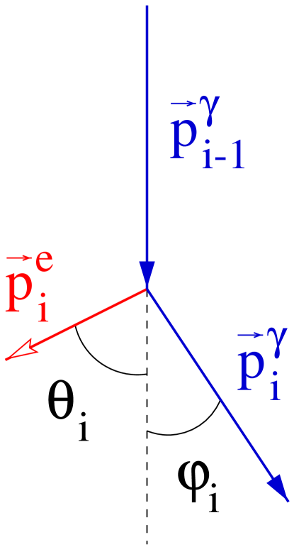
Figure 1: Kinematics of Compton scattering.

In order to overcome the relatively low detection efficiency ($<1\%$) intrinsic of a double scatter Compton telescope such as COMPTEL [1] a homogeneous, self–triggered, three–dimensional (3D) position sensitive detector such as a LXeTPC, was proposed several years ago [2] . In a COMPTEL type telescope the acceptable event topologies are restricted to a single Compton scatter in a first detector layer (converter), followed by absorption of the scattered $\gamma$–ray in a second detector layer (absorber), with the separation between the two layers large enough to order the two interactions by time-of-flight (TOF) measurement. In a homogeneous detector, however, detection of MeV $\gamma$–rays allows a variety of different event topologies to be recorded and used for imaging, with a large increase in efficiency. In absence of a TOF measurement, the correct order of the multiple Compton interactions has to be determined from the redundant kinematical and geometrical information measured for each event. As previously suggested in Aprile et al. 1993 [3] and more recently in Schmid et al. 1999 [5] and in Boggs et al. 2000 [4] , event reconstruction based on Compton kinematic allows to correctly order the interactions. Moreover, background suppression is a direct consequence Compton kinematic reconstruction. Here we present the current status of our work on this topic within the context of the LXeGRIT program.

2 Definition of the problem

The kinematic of Compton scattering is displayed in Fig. 1. Energy and momentum conservation in the Compton scatter process are written as

$$E_{i-1}^{\gamma} = E_{i}^{\gamma}+E_{i}^{\mathrm{e}}$$ (1)

$$\vec{p}_{i-1}^{\gamma} = \vec{p}_{i}^{\gamma}+\vec{p}_{i}^{\mathrm{e}}\qquad(i=1,\ldots,N-1)$$ (2)

with $E_{i}^{\gamma}\;(i=0,\ldots,N-1)$ and $E_{i}^{\mathrm{e}}\;(i=1,\ldots,N)$ the energy of the $\gamma$-photon and the scattered electron after interaction $i$. $E_{0}^{\gamma}$ is the energy of the incoming photon and $\vec{p}_{i}$ are the corresponding momenta. The dispersion relations for photons and electrons reduce these four equations to three independent equations. The vector equation 2 translates into two independent equations for the photon scatter angle $\varphi_{i}$ and the electron scatter angle $\theta_{i}\;(i=1,\ldots,N-1)$:

$$\cos\varphi_{i} = 1-\frac{1}{W_{i}}+\frac{1}{W_{i+1}}\textrm{, with:}\quad W_{i}=\frac{E_{i}}{m_{0}c^{2}}$$ (3)

$$\cot\theta_{i} = \left(1+\frac{E_{i-1}^{\gamma}}{m_{0}c^{2}}\right)\>\tan\frac{\varphi_{i}}{2}$$ (4)

If the last measured interaction $N$ is a photo-absorption, there is no meaningful electron scatter angle $\theta_{N}$ (even though an electron is released in the process). For LXeGRIT, the electron scatter angles are not measured (in the considered energy range, interactions are actually pointlike, since the typical electron range does not exceed the given granularity) and are therefore ignored in the following. The detector measures $N$ energy deposits $E_{i}(\approx E_{i}^{\mathrm{e}})$ and $N$ interaction locations $\vec{x}_{i}$. For a given interaction sequence, the locations determine geometrically $N-2$ photon scatter angles $\varphi^{\triangleleft}$${}_{i}\ (i=2,\ldots,N-1)$ in the usual case of unknown source position:

$$\cos{\varphi^{\triangleleft}}_{i}=\frac{\overrightarrow{u}_{i}\cdot\overrightarrow{u}_{i+1}}{|\overrightarrow{u}_{i}||\overrightarrow{u}_{i+1}|}$$ (5)

where $\overrightarrow{u}_{i}~{}=~{}(x_{i}-x_{i-1},\>y_{i}-y_{i-1},\>z_{i}-z_{i-1})$.
For calibration sources, $\varphi^{\triangleleft}$₁ is known additionally. Moreover, $N-1$ Compton scatter angles $\bar{\varphi}$_i are measured by the energy deposits according to equation 3, noting that $E_{i}^{\gamma}=\sum_{j=i+1}^{N}E_{j}\;(i=0,\ldots,N-1)$. This redundant information allows testing of the sequence of the interaction points based solely on kinematics. A straightforward test statistic consists of summing the differences of the scatter angles quadratically:

$$T_{\varphi}^{\prime}=\sum_{i=2}^{N-1}(\cos{\bar{\varphi}_{i}}-\cos{\varphi^{\triangleleft}_{i}})^{2}$$ (6)

Ideally, the test statistic would be zero for the correct sequence if the photon is fully contained. With measurement errors, $T_{\varphi}^{\prime}$ is always greater than zero, but the correct interaction sequence is still most likely to produce the minimum value of the test statistic. In addition to minimizing $T$, an upper threshold can in principle discriminate against photons that are not fully absorbed. This can be improved by weighting the summands with the measurement errors:

$$T_{\varphi} = \sum_{i=2}^{N-1}\frac{(\cos{\bar{\varphi}_{i}}-\cos{\varphi^{\triangleleft}_{i}})^{2}}{\sigma_{i}^{2}}$$ (7)

$$\textrm{with:}\quad\sigma_{i}^{2} = \sigma_{\cos{\bar{\varphi}},i}^{2}+\sigma_{\cos{\varphi^{\triangleleft}},i}^{2}$$

For each triplet of interactions $\sigma_{\cos{\bar{\varphi}}}$ and $\sigma_{\cos{\varphi^{\triangleleft}}}$ are computed in the following way:

$$\sigma_{\cos{\varphi^{\triangleleft}},i}^{2} = \frac{2}{|\overrightarrow{u}_{i}|^{2}\cdot|\overrightarrow{u}_{i+1}|^{2}}\sum_{k=1}^{3}(2u_{i,k}^{2}+2u_{i+1,k}^{2}-2u_{i,k}u_{i+1,k})\cdot\sigma_{k}^{2}$$ (8)

with: $$k$$ spatial coordinate index and

$$\sigma_{k}$$ position uncertainty on each coordinate

$$\sigma_{\cos{\bar{\varphi}},i}^{2} = \frac{1}{W_{i}^{4}}\cdot\sigma(W_{i}-W_{i+1})^{2}+\left(\frac{1}{W_{i}^{2}}-\frac{1}{W_{i+1}^{2}}\right)^{2}\cdot\sigma(W_{i+1})^{2}$$ (9)

Eq. 8 holds only under assumption that the 3D separation between two interactions is large compared to position uncertainties, which we insure by corresponging data cuts.

3 The LXeGRIT Detector

The LXeGRIT (Liquid Xenon Gamma-Ray Imaging Telescope) instrument was developed as a prototype of Compton telescope exploiting 3D imaging capability and good spectral response of a LXeTPC. It is described in Aprile et al. [6]^, [7] . The principle of operation of the LXeTPC is schematically shown in Fig. 2. The TPC is assembled in a cylindrical vessel of 10 l volume, filled with high purity liquid xenon (LXe). The sensitive area is $20\times 20$ cm² and the drift region is 7 cm. The detector operates over a wide energy range from $\sim$ 200 keV to 20 MeV. Both ionization and scintillation light signals are detected. Ionization signals measure energy and 3D position for each interaction, while the fast ($<5$ ns) Xe scintillation light provides the event trigger. The drift of free ionization electrons in the uniform electric field, typically 1 kV/cm, induces charge signals on a pair of orthogonal planes of parallel wires with a 3 mm pitch, before collection on four independent anodes. Each of the 62 X-wires and 62 Y-wires and each anode is amplified and digitized at a sampling rate of 5 MHz, to preserve the pulse shape. The X-Y coordinate information is obtained from the pattern of hits on the wires, while the energy is obtained from the amplitude of the anode signals. The Z-coordinate is determined from the drift time measurement, referred to the light trigger. Relying on low-noise readout electronics (less than $\sim$ 400 e^- RMS on the wires, $\sim$ 800 e^- RMS on the anodes), the TPC can well detect the multiple interactions of MeV $\gamma$–rays, with a minimum energy deposit as low as 100 keV.
A typical event is displayed in Fig. 3. The digitized signals on all wires and active anodes are shown as a function of drift time. The incoming photon makes two Compton scatterings befor being photoabsorbed. In this 3-interaction event, in fact, the sum of the three anode pulse heights gives 1.8 MeV. The corresponding locations of the interactions are clearly seen on the X-Y wires.
The energy resolution, at 1 kV/cm electric field, has been measured to be $\sim 9\%$ FWHM at 1 MeV, scaling as $1/\sqrt{E}$: the position resolution is $\sim 1$ mm on the X-Y coordinates, as expected for the given granularity (3 mm spaced wires), and 0.15 mm on the Z coordinate, determined by the accuracy on the drift time measurement.
Once digitized, wire and anode signals are passed through a signal recognition and fitting algorithm, which sorts the different event topologies and reduces the event to the relevant information, i.e. X-Y-Z location and energy for each interaction in the sensitive volume.

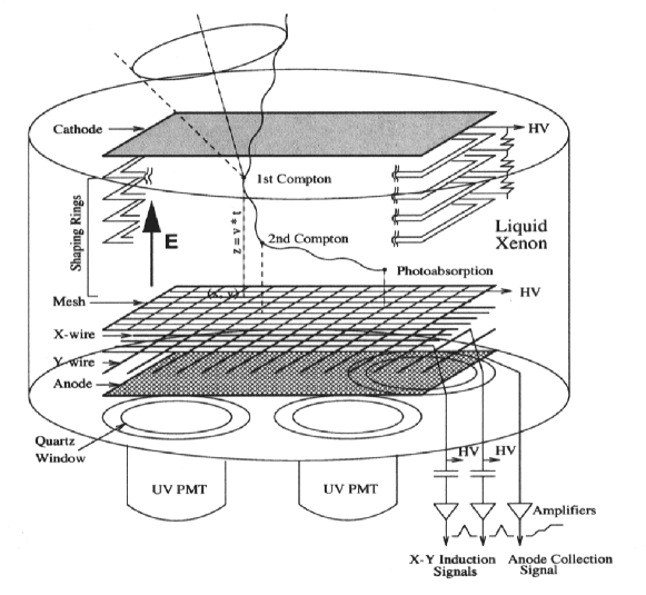
Figure 2: LXeTPC schematic.

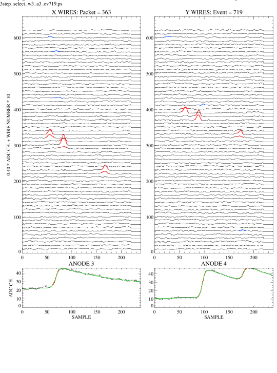
Figure 3: On-line display of a 3-interaction event (two Compton scatters followed by photoabsorption).

4 Performance of the algorithm

The Compton sequence reconstruction (CSR) algorithm has been implemented in a C routine, as a module of the LXeGRIT analysis software. It has been tested using Monte Carlo data and then applied to experimental data.
Given the range of tipically recognizable interactions, $3~{}\leq$ N $\geq~{}6$, the algorithm currently performs a “brute force” search through all N factorial (N!) permutations of the sequence. For each sequence the algorithm first checks whether the sequence is kinematically forbidden (i.e. $\cos{\bar{\varphi}}$_i  $<~{}-1$ ), in which case the sequence is rejected. Otherwise it calculates the test statistic (defined in eq. 7). For each event the sequence which minimizes the test statistic is then selected as the true Compton scattering sequence.
Rejection of non-Compton events or discrimination between fully and partially absorbed photons, based on some upper threshold on the minimum value of the test statistic, is a desirable feature of the algorithm. The topic of background rejection will be discussed elsewhere in a broader contest. In this paper, an upper threshold on the test statistic has been applied only to reduce the fraction of incorrectly reconstructed Compton events.

4.1 Monte Carlo Data

The performance of the algorithm on Monte Carlo data is shown in Figs. 4 and 5. The events have been generated using the GEANT detector simulation package [8]. $\gamma$–rays of different energies have been generated. Here we consider 511 keV  and 1275 keV, i.e. the two lines from ²²Na  decay, 898 keV  and 1836 keV, from ⁸⁸Y (as the two sources have been widely used in calibrating the detector: the source location during data taking has been reproduced in the simulation). Each $\gamma$–ray is tracked through a detailed mass model of the LXeGRIT detector. For each interaction, X-Y-Z location, energy deposit and interaction type are recorded. The following conditions and experimental uncertainties are then imposed on the simulated events to reproduce the LXeGRIT events:

• 100 keV minimum energy threshold for detection of each interaction

• 1 mm RMS position resolution on each coordinate

• 10$\%$ FWHM at 1 MeV, scaling as $1/\sqrt{E}$, energy resolution.

• 5 mm minimum spatial separation on at least one coordinate between each pair of interactions in order to consider two interaction locations mutually resolved. If this condition is not fullfilled the two interactions are clustered and considered as one single interaction

We focus on events with three detected interactions (the minimum number required in the algorithm) since this event class dominates over higher multiplicities in LXeGRIT. Fig. 4 summarizes the results for events in the 1836 keV full-energy peak. On the left panel test statistic for the true sequence and for the remaining five false sequences is shown. The right panel displays the fraction of correctly and incorrectly reconstructed events (efficiency and confusion) as a function of the upper threshold applied to test statistic.
Efficiency, contamination and the fraction of rejected events are shown as a function of energy in Fig. 5 for an upper threshold of 2 on test statistic. For energies larger than 1 MeV a reconstruction efficiency larger than 50$\%$ is achieved.

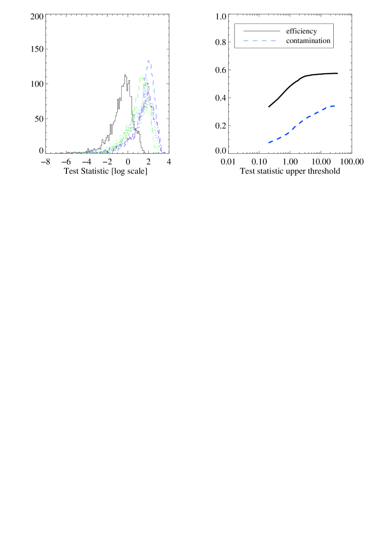
Figure 4: Performance of the CSR algorithm tested with Monte Carlo generated events in the 1836 keV photopeak. Left: the test statistic for the true sequence (continuos line) and for the remaining five false sequences, right: fraction of correctly and incorrectly reconstructed events (efficiency and confusion) as a function of upper threshold on test statistic.

Figure 5: Efficiency, contamination and the fraction of rejected events as a function of energy for an upper threshold of 2 on test statistic.

4.2 Experimental Data

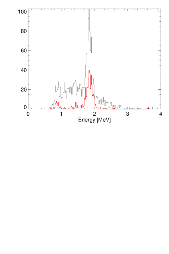
Figure 6: Energy spectrum for an ⁸⁸Y  source at distance, before any selection: the energy spectrum for events in the ARM peak is also shown (thick line).

The CSR algorithm has been tested with a sample of 3–interaction events from an ⁸⁸Y  source (898 and 1836 keV $\gamma$–rays) placed 2 m above the detector. The energy spectrum for all the events in the 3-interaction sample, before applying any selection, is shown in Fig. 6. Since the minimum energy threshold in this sample is $\sim$220 keV (see Fig. 9), the 898 keV line turns out to be largely suppressed. We note here that the minimum detectable energy is determined not only by the detector signal-to-noise conditions, but also by the trigger conditions and event selections applied during data taking. In Fig. 7 the spatial separation between interactions is shown, and in Fig. 8 the corresponding interaction depth. The distribution for the first interaction peaks at high Z (i.e. small interaction depth), while for the second interaction it peaks in the center and it is relatively flat for the third interaction, with the maximum towards the bottom of the detector. This is indeed what is expected for a source on the top of the detector, 2 m away.

Figure 7: Separation in space between interaction locations. Left: first and second interaction, right: second and third interaction. The 3-interaction sequences were ordered by the CSR algorithm.

Figure 8: From left to right: interaction depth for the first, second and third interaction location. The source was placed 2 m above the LXeTPC. 7 cm is the maximum drift length.

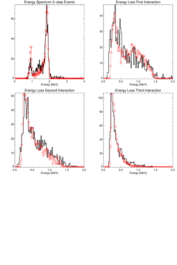
Figure 9: 3-interaction events energy spectra for an ⁸⁸Y source at distance (data selections as described in the text): solid thick line $\rightarrow$ experimental data, diamonds $\rightarrow$ Monte Carlo data. Left top: energy spectrum as obtained summing up, for each event, the energies in the 3 detected interactions (sum-coincidence mode). Right top: energy spectrum for the first interaction. Left bottom: energy spectrum for the second interaction. Right bottom: energy spectrum for the third interaction.

Figure 10: ARM spectrum for 1836 keV photons (3-interaction events): the interaction sequence has been ordered by the CSR algorithm described in the paper. 55$\%$ of the events ends up in the ARM peak within 3$\sigma$’s from zero ($\sim$3 degrees).

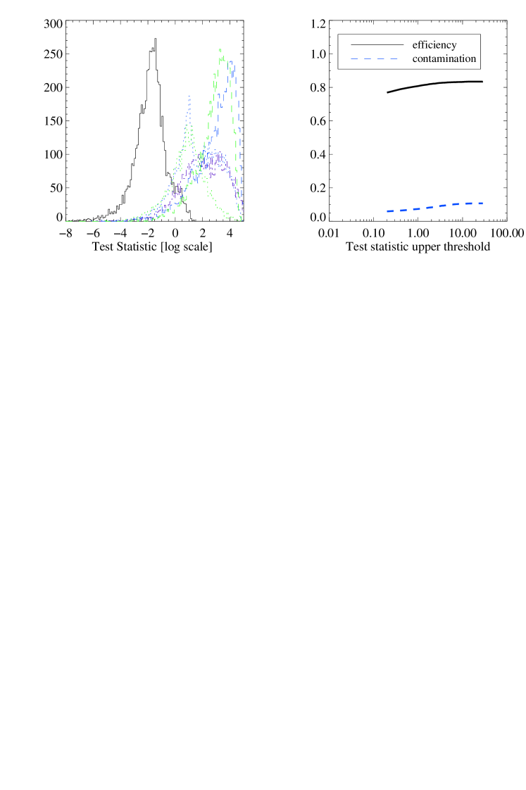
Figure 11: Monte Carlo generated events in the 2000 keV photopeak, for the Xe-ACT described in the text: left: the test statistic for the true sequence (continuos line) and for the remaining five false sequences, right: fraction of correctly and incorrectly reconstructed events (efficiency and confusion) as a function of upper threshold on test statistic.

Exploiting the imaging capability of the detector, we impose a maximum separation of 7 cm between interactions, in order to reject background events. Since the attenuation length in LXe for 1 MeV photon is $\sim$5 cm, separations larger than 7 cm are easily due to pile-up of independent $\gamma$–rays. The impact of this selection can be evaluated comparing the energy spectrum shown in Fig. 6 to the one in Fig. 9, top-left panel, where events with energies exceeding 2 MeV have been effectively rejected, as well as events in the Compton continuum, and the 898 keV line, even with reduced statistics, is clearly detected.
Dealing with experimental data the true Compton sequence is not known a priori, so that, to estimate the performance of the CSR algorithm, we have necessarly to rely on additional information.
As a possible approach to test the performance of the CSR algorithm, we compared experimental to Monte Carlo data (in this case 220 keV energy threshold has been assumed also in the simulation): Fig. 9 separately shows the distribution of the energies deposited in the three interactions, as ordered in a sequence by the CSR algorithm, for the case of ⁸⁸Y  experimental data and for Monte Carlo data for which the true sequence is known. The overall agreement is fairly good: noticeably the three different spectra show significantly distinguishable shape, making the comparison more sensitive.
A more direct approach to test the performance of the algorithm on experimental data is the following: since the source position is known, two indipendent measurements of the first Compton scattering angle are given ($\bar{\varphi}$₁ and $\varphi^{\triangleleft}$₁), translating into the so-called angular resolution measure (ARM), defined as the difference between $\bar{\varphi}$₁ and $\varphi^{\triangleleft}$₁. Fig. 10 shows the resulting ARM distribution obtained with the 3–interaction events in the 1836 keV full energy peak, ordered by the CSR algorithm. For each event within $3~{}\sigma$s of the ARM peak around 0^∘, $\sigma~{}\simeq~{}$3^∘, we assumed the sequence to have been correctly ordered, while larger ARM values are considered wrongly reconstructed sequences.
Imposing an upper threshold of 2 on the test statistic, we obtain 55$\%$ efficiency, in excellent agreement with the value expected from Monte Carlo.
The energy spectrum of these correctly sequenced events is shown in Fig. 6: the Compton continuum and other background events are clearly suppressed.

5 From LXeGRIT to Xe-ACT

A concept based on gas XeTPCs has been recently proposed [9] as a possible candidate for an Advanced Compton Telescope (Xe-ACT), aiming at orders of magnitude improvement over the current sensitivity, and further studies are underway. Going from LXe to high-pressure Xe, a highly improved energy resolution is obtained [10], approaching the theoretical statistical limit. 20 keV FWHM at 1 MeV energy resolution has been conservatively assumed, based on experimental data. Furthermore, in a lower density active medium (e.g. 0.15 g cm^-3 gas vs. 3.06 g cm^-3 for LXe) the average separation between two consecutive interactions is much larger, thus improving angular resolution.
A 2$\times$2$\times$2 m³ active volume detector, filled with 0.15 g cm^-3 Xe, has been simulated. The performance of the CSR algorithm for 2 MeV photons is shown in Fig. 11: an efficiency exceeding 80$\%$ is achieved, with a contamination level $<~{}10\%$.

6 Conclusions

The efficiency of the LXeGRIT instrument as a Compton telescope depends on the capability to order the sequence of multiple Compton interactions detected in the TPC. This capability has been experimentally tested, and we conclude that the true sequence can be efficiently (efficiency $\sim 60\%$ for 1.8 MeV photons) determined, in good agreement with expectations (i.e. Monte Carlo model). The experience gained in operating the LXeGRIT detector also suggests possible ways to improve this performance based on realistic detector conditions.

References

- [1] Schönfelder V., et al., 1993, ApS 86, 657
- [2] Aprile E., et al., 1989, SPIE Vol.1159, 295
- [3] Aprile E., et al., 1993, NIM A 327, 216
- [4] Boggs, S. E. and Jean, P., 2000, A&AS, in press (astro-ph/0005250)
- [5] Schmid, G. J., et al., 1999, NIM A 430, 69
- [6] Aprile E., et al., 1998, NIM A 412, 425
- [7] Aprile E., et al., 2000, in ’Frontiers Detectors for Frontier Physics’ Proceedings, NIM A, special issue, in press
- [8] GEANT, Detector Description and Simulation Tools, CERN Program Library, Long Writeup W5013
- [9] Aprile E., Curioni A., Oberlack U.G., 1999, in Roland Diehl, Dieter Hartmann (eds.) Proc. ’Astronomy with Radioactivities’, MPE report 274 (ISSN 0178-0719),
- [10] Bolotnikov A., Ramsey B.,1997, NIM A 396, 360