Weak Lensing Constraints on Cluster Structural Parameters

Abstract

We study the reliability of dark matter (DM) profile determinations for rich clusters of galaxies based on weak gravitational lensing measurements. We assume that cluster DM density profiles are fully described by two parameters: a scale radius $r_{s}$ and a dimensionless central density $\delta_{c}.$ We consider three functional forms for the mass distribution: a softened isothermal sphere (SIS), and two models proposed on the basis of numerical simulations of CDM universes: the Navarro, Frenk, & White model (NFW) and the Klypin, Kravstov, Bullock, & Primack model (KKBP). A maximum likelihood parametric method is developed and applied to simulated images of background galaxies at z=2.0 lensed by clusters at $z=0.2,$ $0.5,$ and $0.8.$ The images have field size ($\sim 10$ arcmin) and angular resolution ($\sim 0.5$ arcsec) characteristic of the new generation of 8–10 meter-class ground-based telescopes. The method recovers the correct virial mass of the DM halo, $M_{200},$ to within $\sim 10\%$ at all redshifts. The recovered values of $\delta_{c}$ and $r_{s}$ are only accurate to $\sim\,$25%; however, their correlated errors are such that greater accuracy is obtained for the mass. Clusters with an SIS density profile are recognized by the method, while NFW and KKBP clusters are recognized as not being SIS. The method does not discriminate between NFW and KKBP profiles for clusters of a given mass, because they are too similar in their outer regions. Strongly lensed arcs near the cluster centers would be needed to distinguish NFW from KKBP. The accuracy with which $\delta_{c}$ and $r_{s}$ are determined, and the different models are distinguished, improves with increasing redshift because the gravitational potential is sampled out to a larger radius for a given field size. These preliminary results conclude that our maximum likelihood method is a promising candidate for both virial mass measurements and testing numerical predictions of DM halo structures although further tests that include real world effects still remain to be done.

1 Introduction

The study of rich clusters of galaxies, over a range of redshifts out to $z\sim 1,$ has emerged as an important tool for studying structure formation and constraining cosmological parameters (White, Efstathiou, & Frenk 1993; Bahcall & Cen 1993; Carlberg et al. 1997; Bahcall, Fan, & Cen 1997; Riechart et al. 1998; Eke et al. 1998; Girardi et al. 1998; Borgani et al. 1999; Blanchard et al. 2000). The theoretical underpinning of this approach is the Press & Schechter (1974; PS) approximation for the abundance of collapsed objects as a function of mass and redshift in a given cosmological model. The PS formalism is extremely sensitive to cluster virial mass since the fraction of collapsed objects of mass $>M$ is given by the integral of the tail of a Gaussian function with the lower limit of integration dependent on $M$ and cosmological parameters. Therefore, even relatively modest errors in virial mass measurement can drastically affect the derived cosmological parameters (Willick 2000). Accurate virial mass determination is thus of paramount importance.

Observational data for clusters do not, however, directly yield their masses. Instead, they measure related properties such as X-ray luminosity and/or temperature, cluster richness, or velocity dispersion. To date, efforts to constrain cosmological parameters using clusters have been based mainly on either X-ray temperature/luminosity (Girardi et al. 1998; Donahue et al. 1998; Sadat, Blanchard, & Oukbir 1998; Riechart et al. 1998; Borgani et al. 1999; Blanchard et al. 1999), or velocity dispersion (Carlberg et al. 1998; Tran et al. 1999) measurements as mass indicators. However, the accuracy of such mass estimates is open to question. They depend on assumptions of hydrostatic equilibrium of the hot intracluster gas and virial equilibrium of cluster galaxies, respectively, which may not hold in a given cluster. It is thus important that alternative mass estimators, independent of the assumption of hydrostatic or virial equilibrium, also be applied when possible.

Weak gravitational lensing of background sources by clusters is perhaps the most attractive such alternative (see Narayan & Bartelmann 1999, hereafter NB99, and Bartelmann & Schneider 1999, hereafter BS99, for recent reviews). While strong lensing, in which large arcs or multiple images of a single source are produced, can provide precise measurements of the mass in the inner regions ($r\lower 2.15277pt\hbox{$\,\buildrel<\over{\sim}\,$}200h^{-1}\!$ kpc) of clusters (e.g., Tyson, Kochanski, & Dell’Antonio 1998), it does not constrain the virial mass of clusters, which typically corresponds to radii of 1–2$h^{-1}\!$ Mpc. In contrast, weak lensing, which consists of small but coherent distortions of background galaxy shapes, can be detected statistically out to several $h^{-1}\!$ Mpc. Cluster mass estimates have now been obtained from weak lensing data by a number of groups (e.g., Tyson, Valdes, & Wenk 1990; Kaiser & Squires 1993, 1996; Smail et al. 1997; Squires et al. 1997; Hoekstra et al. 1998; Luppino & Kaiser 1997). These estimates have generally been found to agree well with the X-ray and velocity dispersion mass estimates (Lewis et al. 1999; Willick 2000).

Several of the these weak lensing studies were done with the Hubble Space Telescope (HST) whose superb imaging capabilities ensure that it will play an important role in future projects as well. However, the primary observational driver for future work is likely to be improvements in the capabilities of the new generation of large aperture ground-based telescopes. Wide field ($\sim 10^{\prime}$–1^∘) imaging CCD cameras have recently or will soon come on line (see, e.g., Luppino, Tonry, & Stubbs 1998; Kaiser, Tonry, & Luppino 2000) at telescopes with excellent image quality ($\lower 2.15277pt\hbox{$\,\buildrel<\over{\sim}\,$}0.5^{\prime\prime}$ seeing), such as CFHT, Subaru, Magellan, VLT, and Gemini. These instruments are extremely well-suited to weak-lensing studies. In particular, they will fully cover the field of moderate-redshift ($0.2\lower 2.15277pt\hbox{$\,\buildrel<\over{\sim}\,$}z\lower 2.15277pt\hbox{$\,\buildrel<\over{\sim}\,$}1$) clusters, with data that probe out to and beyond the virial radius.

The problem of cluster mass “inversion”, i.e. reconstruction of the mass as a function of position from weak lensing data, has received considerable attention in recent years (e.g., Kaiser & Squires 1993; Seitz & Schneider 1997; Bartelmann 1998). Most of these efforts have aimed at nonparametric mass reconstructions, in which no a priori assumptions are made about the underlying mass distribution. However, there is evidence from numerical simulations that the dark matter distribution in virialized haloes might be well described by simple parametric models. Navarro, Frenk, & White (1997; NFW) have proposed a model (§2) that has received perhaps the most attention. Recent high-resolution simulations have suggested departures from the NFW model at small radii, leading Kravstov, Klypin, Bullock, & Primack (1998; KKBP) to propose an alternative parameterization. Recent efforts to distinguish between these alternatives using the rotation curves of dwarf galaxies have been inconclusive (van den Bosch & Swaters, 2000), leaving it an open problem. The NFW and KKBP distributions are, however, similar at radii encompassing $\lower 2.15277pt\hbox{$\,\buildrel>\over{\sim}\,$}10\%$ of the virial mass, where both may be described as locally power-law profiles $\rho(r)\propto r^{-\gamma},$ where $\gamma$ varies slowly from $\lower 2.15277pt\hbox{$\,\buildrel<\over{\sim}\,$}2$ near a characteristic radius $r_{s}$ to $3$ at $r\gg r_{s}.$ In this sense, NFW and KKBP differ distinctly from the generic softened isothermal sphere (SIS) model, in which $\rho(r)\propto r^{-2}$ at all radii beyond a small inner core. The SIS model yields the flat rotation curves characteristic of spiral galaxies, and thus has often been viewed as a reasonable representation of equilibrium dark halos.

Given the findings by NFW and KKBP that dissipationless gravitational clustering may produce simple and universal mass distribution laws, a strong case can be made for using weak lensing to constrain the parameters of such laws. This approach would complement the existing methods of nonparametric mass inversion. Fitting parametric models has advantages and disadvantages. The chief advantage is that, if the model is correct or nearly so, a parametric approach is robust against random error in the presence of noise. The obvious disadvantage is that the method may not flag an incorrect model. Nonetheless, we believe that the case for universal density profiles is strong enough that it amounts to a “theoretical prediction” which can and should be fit to the data.

This paper has two objectives, to see if we can distinguish between several theoretically motivated density profiles using weak lensing data; and second, to ascertain how accurately we can measure virial masses from such data. We adopt three trial parameterizations of cluster masses: SIS, NFW, and KKBP (see § 2 for details), and simulate lensed fields for each of these mass distributions, for clusters of varying mass and redshift. We then apply our maximum likelihood method to these simulations (§ 3). For each cluster of a given profile type, we compute the likelihood with respect to the parameters of that profile type and of the other two, allowing us not only to constrain the parameters but to test whether we can discriminate among the models. One of our key conclusions is that we can indeed distinguish the SIS from NFW or KKBP, but not NFW from KKBP. This is important, because a basic prediction of the Cold Dark Matter (CDM) hypothesis is that halo mass distributions depart from an $r^{-2}$ law in their outer regions. Our work shows that this prediction is testable via weak lensing data.

In addition to developing a method to test theoretical predictions of cluster mass profiles, our work has another, more basic, goal, already alluded to in the first paragraph. For clusters to be used as cosmological probes via the PS or related formalisms, one must determine their virial masses with high accuracy. In the PS formalism, the term virial mass has a very specific meaning: it is the mass contained within a sphere whose mean interior density is a particular multiple, $\delta_{V},$ of the mean density of the universe. The quantity $\delta_{V}$ depends on cosmological parameters and on redshift. Since the former are not known a priori—and indeed may be the goal of our study—one needs to be able to express mass as a function of radius in a flexible way. This cannot be done independently of a model for the density profile of the cluster; moreover, once a model is adopted, its defining parameters must be reasonably well-known to obtain a virial mass for a given choice of cosmological parameters (see, e.g., Willick 2000 for a detailed discussion).

The outline of this paper is as follows: Section 2 and 3 introduce the basic lensing formalism and our parametric maximum likelihood inversion method. We then discuss the simulations used to test the method in Section 4, and Section 5 presents the results of these simulations. Section 6 discusses the basic conclusions and directions for further research. A derivation of the shear and magnification for SIS, NFW and KKBP clusters is in Appendix 1, whereas Appendix 2 considers the computation of the virial mass for a cluster with known structural parameters.

2 Basic Formalism

In this section we derive expressions for lensing angle, convergence, and shear for two-parameter, spherically symmetric mass distributions such as SIS, NFW, and KKBP. Such mass profiles are characterized by a density scale $\rho_{c}$ and a scale length $r_{s}.$ We follow NFW in writing $\rho_{c}=\rho_{crit}\,\delta_{c},$ where $\rho_{crit}=3H_{0}^{2}/8\pi G,$ and thus write the density law as

$$\rho(r)=\rho_{crit}\,\delta_{c}\,\eta(r/r_{s})\,,$$ (1)

where the function $\eta(x)$ characterizes the shape of the density profile. For the three mass distributions considered in this paper we have

$$\eta(x)=\left\{\begin{array}[]{ll}(1+x^{2})^{-1}&{\rm(SIS)}\\ x^{-1}(1+x)^{-2}&{\rm(NFW)}\\ x^{-0.2}(1+x^{2})^{-1.4}&{\rm(KKBP).}\end{array}\right.$$ (2)

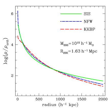
Figure 1: Mass density, in units of the critical density, plotted as a function of radius for three clusters each with $M_{200}=10^{15}h^{-1}\!M_{\odot}.$ One cluster has an SIS density profile, one has an NFW profile, and one has a KKBP profile. The cluster structural parameters $r_{s}$ and $\delta_{c}$ are chosen to make the three clusters as similar as possible. See text for further details.

Figure 1 shows these three profiles for the case of a cluster with virial mass $M_{200}=10^{15}h^{-1}M_{\odot}$ and virial radius $R_{200}=1.63h^{-1}Mpc$, for $\delta_{v}=200$. Spherical symmetry implies circular symmetry on the sky. The lensing angle, $\alpha(\theta)$ must be purely radial, dependent only on $\theta$, the angle on the sky from the center of the mass distribution. Furthermore circular symmetry implies (e.g., NB99) that

$$\alpha(\theta)=\frac{4GM(\theta)}{c^{2}\theta}\frac{D_{LS}}{D_{L}D_{S}}\,,$$ (3)

where $M(\theta)$ is the mass enclosed within a circle of angular radius $\theta,$ and the various $D$’s are angular diameter distances. The subscript $L$ refers to the lens, i.e., the cluster, and the subscript $S$ to the source, i.e, the object being lensed. For reference, we write down expressions for these distances as a function of redshift. We follow the notation of Peebles (1993) for cosmological quantities, except that we use the subscript $M$ rather than $0$ to denote the mass density parameter. For $D_{L}$ ($D_{S}$) we have

$$D(z)=\frac{c}{H_{0}}\,\frac{y(z)}{1+z}$$ (4)

where $z$ is the lens (source) redshift, and $y(z)$ is given, in the case of a flat ($\Omega_{\rm M}+\Omega_{\Lambda}=1$) universe, by

$$y(z)=\int_{0}^{z}\frac{dz^{\prime}}{\sqrt{\Omega_{\rm M}(1+z^{\prime})^{3}+\Omega_{\Lambda}}}\,.$$ (5)

The lens-source angular size distance is

$$D_{LS}=\frac{c}{H_{0}}\,\frac{y_{{}_{LS}}}{1+z_{{}_{S}}}\,,$$ (6)

where we have introduced the abbreviations $y_{{}_{L}}=y(z_{{}_{L}}),$ $y_{{}_{S}}=y(z_{{}_{S}}),$ and $y_{{}_{LS}}=y_{{}_{L}}-y_{{}_{S}}$ (again, assuming a flat universe). Using the above expressions, we have

$$\frac{D_{LS}}{D_{L}D_{S}}=\frac{H_{0}(1+z_{{}_{L}})}{c}\,\frac{y_{{}_{LS}}}{y_{{}_{L}}y_{{}_{S}}}$$ (7)

This last form of the distance ratio will be useful in what follows.

Adopting the two-parameter density profile (Eq. 1), the projected mass within an angle $\theta$ on the sky is given by

$$M(\theta)=2\pi\int_{0}^{D_{L}\theta}\!r\,dr\int_{-\infty}^{\infty}\rho\left(\sqrt{r^{2}+z^{2}}\right)dz$$

$$=4\pi\rho_{crit}\,\delta_{c}D_{L}^{3}\theta_{s}^{3}\int_{0}^{\theta/\theta_{s}}\!y\,dy\int_{0}^{\infty}\eta\left(\sqrt{y^{2}+x^{2}}\right)dx\,,$$ (8)

where

$$\theta_{s}\equiv r_{s}/D_{L}$$ (9)

is the halo scale length in angular units. Combining Eqs. 3, 7, and 8, and using the definition of the critical density, we obtain, after some algebra, the deflection angle:

$$\alpha(\theta)=6\,\delta_{c}\,\theta_{s}^{2}\,{\cal Y}(z_{{}_{L}},z_{{}_{S}})\left(\theta/\theta_{s}\right)^{-1}\beta(\theta/\theta_{s})\,,$$ (10)

where

$$\beta(x)\equiv\int_{0}^{x}y\,dy\int_{0}^{\infty}\!\eta\left(\sqrt{y^{2}+w^{2}}\right)dw$$ (11)

and

$${\cal Y}(z_{{}_{L}},z_{{}_{S}})\equiv\left(\frac{y_{{}_{LS}}}{y_{{}_{S}}}\right)\left(\frac{y_{{}_{L}}}{1+z_{{}_{L}}}\right)^{2}\,.$$ (12)

Eqs. 10 and 11 determine the lensing angle for any adopted (spherically symmetric) density law. Note that the lens and source redshifts enter only through the multiplicative factor ${\cal Y}(z_{{}_{L}},z_{{}_{S}}),$ while the shape information is contained entirely in the function $\beta(x).$

2.1 Convergence and Shear

Our formula for $\alpha(\theta)$ enables us to calculate two other important quantities, the convergence $\kappa$ and shear $\gamma.$ To obtain the former, note that

$$\kappa=\frac{1}{2}\nabla\cdot\vec{\alpha}\,=\,\frac{1}{2}\left[\frac{d\alpha}{d\theta}+\frac{\alpha}{\theta}\right]\,,$$ (13)

where the last equality follows from circular symmetry. Using Eq. 10 in Eq. 13, we obtain

$$\kappa(x)=3\delta_{c}\theta_{s}{\cal Y}(z_{{}_{L}},z_{{}_{S}})\left[x^{-1}\beta^{\prime}(x)\right]\,,$$ (14)

where $x=\theta/\theta_{s}.$

The complex shear, $\gamma=\gamma_{1}+{\rm i}\gamma_{2},$ is given by

$$\gamma_{1}=\frac{1}{2}\left(\psi_{,xx}-\psi_{,yy}\right)$$ (15)

and

$$\gamma_{2}=\psi_{,xy}$$ (16)

where $\psi(\theta)$ is the lensing potential (NB99) defined by $\vec{\alpha}=\nabla\psi,$ and the comma signifies partial differentiation. Circular symmetry implies that $\alpha=\psi^{\prime},$ giving, after some manipulation,

$$\gamma_{1}=\frac{1}{2}\cos 2\phi\left[\frac{d\alpha}{d\theta}-\frac{\alpha}{\theta}\right]$$ (17)

and

$$\gamma_{2}=\frac{1}{2}\sin 2\phi\left[\frac{d\alpha}{d\theta}-\frac{\alpha}{\theta}\right]$$ (18)

where $\phi$ is the angle between the radial direction and the $x$-axis. The shear amplitude is

$$|\gamma|=\sqrt{\gamma_{1}^{2}+\gamma_{2}^{2}}=(\alpha^{\prime}-\alpha/\theta)/2$$

$$=3\delta_{c}\theta_{s}{\cal Y}(z_{{}_{L}},z_{{}_{S}})\left[x^{-1}\beta^{\prime}(x)-2x^{-2}\beta(x)\right]\,,$$ (19)

where as before $x=\theta/\theta_{s}$ and Eq. 10 has once again been used.

Note that Eqs. 17 and 18 imply that for $\phi=0$ (i.e., a point along the $x$-axis), $\gamma_{1}=|\gamma|$ and $\gamma_{2}=0.$ However, because of the circular symmetry of the problem, there is no natural orientation for the two Cartesian axes. Thus, we may reinterpret the above equations as saying that at any point, we may adopt a local Cartesian coordinate system in which one axis points along the radial direction, the other along the tangential direction. With respect to such a system, the real part of $\gamma$ is always equal to $|\gamma|$ as given by Eq. 19, while the imaginary part vanishes. As described below, we can measure complex galaxy ellipticities relative to such local axes. The resulting simplification in the probability distribution of observed ellipticities is described in § 3.

2.2 Discussion

The formalism described above shows that the relevant quantities for a lensing analysis—the bending angle $\alpha,$ the convergence $\kappa,$ and the shear $\gamma$—are determined (up to cosmological factors) by three quantities: the dimensionless central density $\delta_{c},$ the scale radius $r_{s},$ and the dimensionless projected mass function $\beta(x)$ given by Eq. 11. The last quantity depends only on the assumed form of the mass distribution (SIS, NFW, KKBP, or other); the former two may then be viewed as parameters to be determined by the lensing analysis. In Appendix 1, we derive expressions for $\beta(x)$ for SIS, NFW, and KKBP.

In Figure 2, we compare the resultant forms of $\alpha(\theta),$ $\kappa(\theta),$ $\gamma(\theta),$ and $M(\theta)$ for a fiducial cluster of virial mass $10^{15}h^{-1}\!M_{\odot}$ lying at $z=0.5.$ The parameters $\delta_{c}\approx 27000$ and $r_{s}=200h^{-1}\!$ kpc were adopted for the NFW profile, while for SIS we took the core radius to be $10h^{-1}\!$ kpc. The parameters for KKBP were determined by requiring that the logarithmic slope of the density profile, $d\ln\rho/d\ln r,$ take on the value $-2$ at $r=200h^{-1}\!$ kpc, where the NFW logarithmic slope has that value as well. These conditions plus fixing the virial mass at $10^{15}h^{-1}\!M_{\odot}$ uniquely determines the profiles and makes the comparison well-defined.

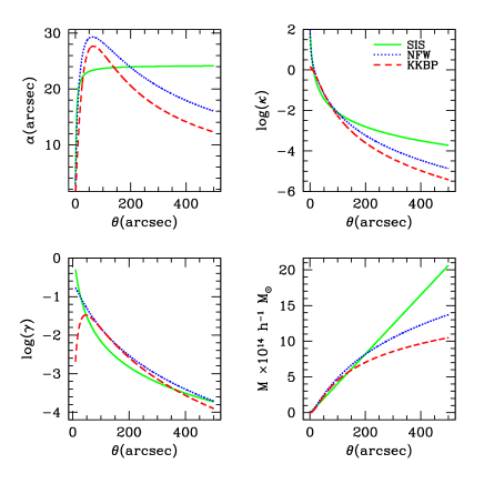
Figure 2: Lensing angle $\alpha,$ convergence $\kappa,$ shear amplitude $\gamma,$ and enclosed mass $M$ plotted as functions of $\theta,$ the angle on the sky from the center of the mass distribution, for a cluster of virial mass $10^{15}h^{-1}\!M_{\odot}$ at a redshift of $0.5.$ Each quantity is shown for each of the three density profiles studied in this paper: SIS, NFW, and KKBP. The three profiles were “matched” as described in the main text. Note that the parameters are the same as those in Figure 1.

3 Maximum-Likelihood Method for Determining Halo Parameters

3.1 Preliminaries

The method is based on the (complex) ellipticities, $\mbox{\boldmath$\epsilon$},$ of galaxy images, computed from the intensity moments $Q_{ab}$,

$$\mbox{\boldmath$\epsilon$}=\epsilon_{x}+i\epsilon_{y}=\frac{Q_{xx}-Q_{yy}+2iQ_{xy}}{Q_{xx}+Q_{yy}}$$ (20)

where

$$Q_{ab}=\frac{\int I\,a\,b\,dy\,dx}{\int I\,dy\,dx}\,,$$ (21)

and $I$ is the measured intensity. As noted above, the formalism is considerably simplified if we transform to a coordinate system in which the real axis (axis 1) points along the tangential direction, and the imaginary axis (axis 2) along the radial direction, with respect to a radial vector joining the lens center and the galaxy. This transformation is accomplished by a simple rotation,

$$\left(\!\begin{array}[]{c}\epsilon_{1}\\ \epsilon_{2}\end{array}\!\right)=\left(\!\begin{array}[]{rr}\sin 2\phi&\cos 2\phi\\ -\cos 2\phi&\sin 2\phi\end{array}\!\right)\left(\!\begin{array}[]{c}\epsilon_{x}\\ \epsilon_{y}\end{array}\!\right)$$ (22)

where $\phi$ is the angle between the original $x$-axis and the real axis at the position of the galaxy.

The ellipticity components $\epsilon_{1}$ and $\epsilon_{2}$ transform under lensing in a particularly simple way. As shown by Miralda-Escudé (1991, hereafter ME91), the ellipticity components of the lensed image (subscript “$L$”) are related to those of the source image (subscript “$S$”) by the transformations

$$\epsilon_{L1}=\frac{\delta+\epsilon_{S1}}{1+\delta\epsilon_{S1}}$$ (23)

and

$$\epsilon_{L2}=\frac{(1-\delta^{2})^{1/2}\epsilon_{S2}}{1+\delta\epsilon_{S1}}\,.$$ (24)

In Eqs. 23 and 24, $\delta$ is the distortion defined by (e.g., ME91)

$$\delta=\frac{1-q_{c}^{2}}{1+q_{c}^{2}}\,,$$ (25)

where

$$q_{c}=\frac{1-(\kappa+\gamma)}{1-(\kappa-\gamma)}$$ (26)

and $\kappa$ and $\gamma$ are the convergence and shear amplitude, respectively.

Our method requires that we invert these transformations to obtain the source ellipticity as a function of the image (lensed) ellipticity. This yields

$$\epsilon_{S1}=\frac{-\delta+\epsilon_{L1}}{1-\delta\epsilon_{L1}}$$ (27)

$$\epsilon_{S2}=\frac{(1-\delta^{2})^{1/2}\epsilon_{L2}}{1-\delta\epsilon_{L1}}\,.$$ (28)

The Jacobian of the inverse transformation is given by

$${\cal J}=\left(\frac{\sqrt{1-\delta^{2}}}{1-\delta\epsilon_{L1}}\right)^{3}\,.$$ (29)

3.2 Probability Distributions

We seek an expression for the probability that the image of a background galaxy will exhibit ellipticity components $(\epsilon_{1},\epsilon_{2})$ (we drop the subscript $L$ in what follows). Following the work of Seitz & Schneider (1995,1996; see also Schneider & Seitz 1995), we write the probability density in terms of the image ellipticity components as

$$p(\epsilon_{1},\epsilon_{2};\delta)=\phi\!\left[\epsilon_{S}(\epsilon_{1},\epsilon_{2};\delta)\right]\times{\cal J}(\epsilon_{1};\delta)\,,$$ (30)

where $\epsilon_{S}\equiv\sqrt{\epsilon_{S1}^{2}+\epsilon_{S2}^{2}},$ and $\epsilon_{S1}$ and $\epsilon_{S2}$ are calculated from the inverse transformation, Eqs. 27 and 28. The function $\phi(\epsilon_{S})$ is the distribution of intrinsic source ellipticities; it only depends on amplitude because of the assumed isotropy of source galaxy orientations, and is normalized by

$$2\pi\int_{0}^{1}d\epsilon\,\phi(\epsilon)=1\,.$$ (31)

A successful application of the maximum-likelihood method requires an accurate model for $\phi(\epsilon).$ We discuss this further in § 6.

The data set with which we maximize likelihood consists of $N$ lensed galaxy images, each with a measured complex ellipticity $\mbox{\boldmath$\epsilon$}_{i}.$ We define the likelihood for the data set as

$${\cal L}=-\sum_{i=1}^{N}\log p(\mbox{\boldmath$\epsilon$}_{i};\delta_{i}(\delta_{c},\theta_{s}),\theta_{i})$$ (32)

where the individual probabilities are given by Eq. 30. Here we have explicitly indicated the dependence of the probability on $\theta_{i},$ the angle between the radius vector connecting the cluster center to the galaxy and the $x$-axis, which is needed for calculating $\epsilon_{1}$ and $\epsilon_{2}$ from the directly measured components $\epsilon_{x}$ and $\epsilon_{y}$ (cf. Eq. 22). The likelihood is maximized with respect to the cluster structural parameters $\delta_{c}$ and $\theta_{s}=r_{s}/D_{L}$.

4 Simulating Lensed Background Fields

In order to quantify the feasibility of the described method, we applied it to synthetic data sets, that covered a wide area in parameter space. These simulations are described in this section; the results are presented in the following section.

The simulations involved generating $10$ fields of galaxies, $10^{\prime}$ on a side with a resolution of $0.3^{\prime\prime}$ per pixel. Each field had approximately $1500$ galaxies randomly distributed per field with an intrinsic ellipticity distribution given by ME91

$$p(q)dq\propto(1+cq)\exp\left[-\left(\frac{q_{1}}{q}\right)^{2}\right]$$

$$\times\left[1-\exp\left(-\frac{1-q}{q_{2}}\right)\right]dq\,,$$ (33)

where $q$ is the ratio of minor to major axes, $q=b/a$ and with $c=0.2$,$\,q_{1}=0.4$ and $q_{2}=0.02$. This probability distribution is shown in Figure 3. The choice of this functional form and the particular parameters for the ellipticity distribution is a best fit (ME91) to the ellipticity distribution of the deep CCD survey (Tyson 1988, Tyson & Seitzer 1988) while the number of galaxies was chosen such that the number of galaxies per unit area is characteristic of real images.

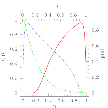
Figure 3: The intrinsic ellipticity distribution. The solid line shows $p(q)$ (Eq. 33) , the dotted line shows the corresponding $p(e)$ while the dashed line shows the observed distribution $p_{obs}(e)$ (Eq. 35). An arbitrary normalization is chosen. The effects of pixelization, increasing the number of galaxies with low ellipticities is also evident.

Each of these $10$ fields were assumed to be at a redshift $z=2.0$ in a  $\Omega_{m}=0.3$,$\,\Omega_{\Lambda}=0.7,h=0.7$ universe. We added uniform Poisson photon noise to each of the images, but ignored the effects of a redshift distribution and seeing for simplicity. We realize that the latter should be included at a later stage. An example of a background field is shown in Figure 4.

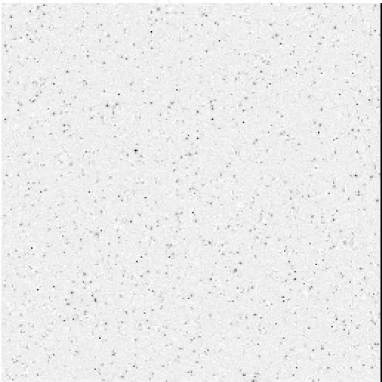
Figure 4: A sample field of background galaxies, seen as they would be in the complete absence of gravitational lensing.

Each of these fields was lensed by dark matter haloes of virial masses $5.0$,$\,7.5$, $10.0$ and $15.0\times 10^{14}M_{\odot}$ each located at redshifts of $z=0.2$,$\,0.5$ and $0.8$. For each halo of a given mass, we simulated three different density profiles, SIS, NFW and KKBP, to study variations with mass, redshift, and profiles. The choice of the particular profiles enabled us to test the algorithm’s discriminatory power at varying scales since the KKBP profile differs from NFW only at small radii while both differ from SIS at all length scales.

However, since all the profiles are two parameter models, specifying the mass does not uniquely determine the values of both parameters. Recognizing that the halo scale length (for NFW and KKBP) and the cluster core radius (SIS) are parameters that lack significant physical significance, we fixed those parameters in our simulations. The scale lengths for SIS and NFW were arbitrarily set to $10$ kpc and $200$ kpc respectively. To determine the scale length for KKBP, we matched the radius at which $d\log\rho/d\log r=-2$ with that for NFW; this fixed the $r_{KKBP}=r_{NFW}/\sqrt{1.8}=149.07$ kpc. This determined the second parameter, the overdensity $\delta_{c}$ or the velocity dispersion $\sigma_{v}$, for a halo of a given mass uniquely.

The actual lensing used an algorithm described in Wilson et al.(1996); it involved solving the lens equation

$$\beta=\theta-\alpha(\theta)$$ (34)

where $\beta$ is the radial position of the unlensed image, $\theta$ is the radial position of the lensed image and $\alpha(\theta)$ is the lensing angle, for every point on the image frame and mapping it to the source frame, thereby correctly handling multiply imaged sources. Examples of these lensed images are shown in Figures 5, 6 and 7. The frames were analyzed using the FOCAS image software (Valdes, 1982) which extracted both the positions and isophotal moments required for the mass inversion. These were then analyzed using the method outlined previously, the results of which are now discussed.

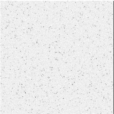
Figure 5: The same field lensed with an SIS halo of mass $m=1.0\times 10^{15}M_{\odot}$ at $z=0.5.$

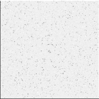
Figure 6: The same field lensed with an NFW halo of mass $m=1.0\times 10^{15}M_{\odot}$ at $z=0.5.$

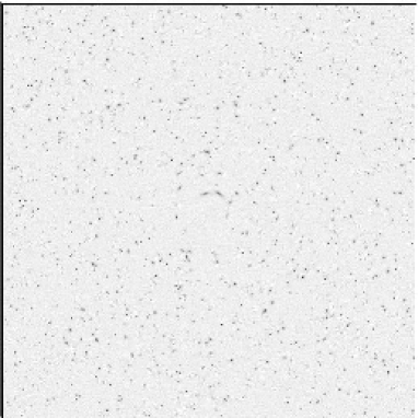
Figure 7: The same field lensed with an KKBP halo of mass $m=1.0\times 10^{15}M_{\odot}$ at $z=0.5.$

5 Results

5.1 Implementation

Before proceeding with the results of the simulation, we briefly describe the actual implementation of the maximum likelihood method, whose formalism was discussed in § 3. In what follows, we assume that the images have been suitably processed with extracted galaxy positions and ellipticities.

An essential element of the maximum likelihood routine is the intrinsic ellipticity distribution of galaxies. Instead of directly using the distribution we used to generate the background fields (Eq. 33), we simulated 10 background fields of galaxies (independent of those used in the actual simulations) and used a fit to the observed ellipticity distribution as the intrinsic ellipticity distribution. The best fit obtained was (see also Figure 3)

$$P(\epsilon_{S})\,d\epsilon_{S}\propto\exp(-1.75866(\epsilon_{S}+1.1388)^{2})$$ (35)

with the constant of proportionality determined by the normalization of the probability function. Note that this is not directly related to Eq. 33 since pixelization and other observational effects have been convolved into it. We discuss this in more detail later in this section.

Each lensed image was analyzed by constructing the likelihood function (Eq. 38) on a $\delta_{c}$-$\theta_{s}$ ($\sigma_{v}$-$\theta_{s}$ for SIS analyses) grid assuming the three (NFW, SIS, KKBP) models in turn. For these three types of analyses, an expectation value for the mass enclosed in a radius of $1.5$ Mpc was computed by weighting the mass obtained at every point on the $\delta_{c}$- $\theta_{s}$ grid by its corresponding probability, summing and dividing by a suitable normalization constant,

$$\langle M_{1500}\rangle=\frac{\sum p(\delta_{c},\theta_{s})M_{1500}(\delta_{c},\theta_{s})}{\sum p(\delta_{c},\theta_{s})}$$ (36)

where $M_{1500}$ is the mass at $1.5$ Mpc and $p(\delta_{c},\theta_{s})$ is the probability function. We chose a fixed radius for the mass computation to compare the accuracy of mass estimation even if the incorrect model was assumed for the analysis. In the case where the virial mass is desired, an appropriate formalism is discussed in Appendix B.

The parameter estimation and profile identification used more direct methods. The location and value of the maximum of the likelihood function determined the parameters $(\delta_{c},\theta_{s})_{ML}$. The profile type was determined by choosing the model with the greatest probability. The following sections summarize the results thus obtained.

5.2 Profile Identification

Table I: Profile Identification Fractions Profile Type Redshift Mass ($10^{15}M_{\odot}$) $0.5$ $0.75$ $1.0$ $1.5$ SIS 0.2 1.0 1.0 0.8 0.9 0.5 0.9 0.7 0.9 0.8 0.8 0.8 0.8 0.8 0.8 NFW 0.2 0.5 0.4 0.2 0.4 0.5 0.6 0.3 0.3 0.5 0.8 0.5 0.1 0.5 0.7 KKBP 0.2 0.5 0.6 0.7 1.0 0.5 1.0 1.0 1.0 0.7 0.8 0.8 0.9 1.0 0.7 NFW+ 0.2 0.5 0.5 0.55 0.85 KKBP 0.5 0.85 0.8 0.9 0.85 0.8 0.7 0.65 0.95 0.95 0.5 0.75 1.0 1.5

Table 1: The fraction of dark matter profiles identified correctly, at the specified redshifts and masses. The NFW+KKBP category is the fraction of clusters correctly identified as not being SIS.

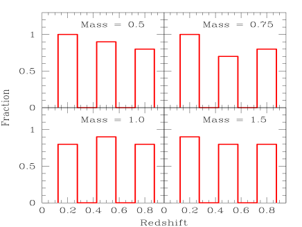
Figure 8: The fraction of SIS clusters correctly identified as such. The masses are all $\times 10^{15}M_{\odot}$.

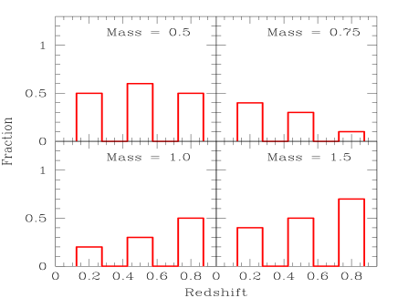
Figure 9: The fraction of NFW clusters correctly identified as such. The masses are all $\times 10^{15}M_{\odot}$.

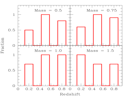
Figure 10: The fraction of KKBP clusters correctly identified as such. The masses are all $\times 10^{15}M_{\odot}$.

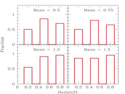
Figure 11: The fraction of clusters correctly identified as not being SIS. The masses are all $\times 10^{15}M_{\odot}$.

The profile identification results are summarized in Table 1 and Figures 8 to 11. We found it instructive to consider the identification of all three profiles separately as well as the ability to distinguish between the SIS and the NFW/KKBP profiles jointly. This was motivated by the similarities between the NFW and KKBP profiles, which differ only in the inner core, an area where weak lensing is not very sensitive.

As is apparent from the data, our method appears to correctly distinguish SIS clusters from the NFW/KKBP joint profile; the correctly identified fraction being approximately $80\%$ for clusters at $z=0.8$. At low redshifts, both NFW and KKBP clusters are misidentified as SIS while at higher redshifts, NFW clusters tend to be misidentified as KKBP. This implies that our method is, as expected, unable to distinguish between the NFW and KKBP profiles, especially at high redshifts. This can be traced to the fact that the two profiles only differ in their innermost regions, evident from Figure 1. However, weak lensing is not sensitive to these regions of the cluster, and so to distinguish between such clusters, we must fall back to strong lensing results. We discuss this further in § 6. For clusters at low redshifts, the lensing data does not extend to a large enough radius to be sensitive to the change in slope of the NFW and KKBP profiles. Accordingly, a greater number are misidentified as SIS.

5.3 Mass Estimation - I

Table II: Mass Estimation - I Profile Type $M_{1500}$ ($10^{15}M_{\odot}$) Redshift 0.2 0.5 0.8 SIS 0.575 0.549 0.550 0.545 0.754 0.715 0.727 0.731 0.914 0.901 0.875 0.873 1.197 1.186 1.191 1.169 NFW 0.550 0.515 0.511 0.510 0.756 0.710 0.724 0.703 0.951 0.906 0.882 0.922 1.318 1.298 1.291 1.223 KKBP 0.546 0.512 0.503 0.502 0.675 0.646 0.628 0.625 0.800 0.757 0.741 0.742 1.037 0.990 1.009 0.957 0.2 0.5 0.8

Table 2: The mean estimated values for $M_{1500}$ if we assume that the profile was correctly identified.

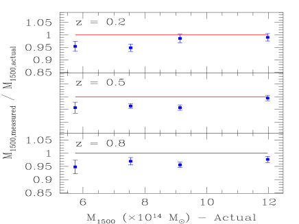
Figure 12: The ratio of the estimated mean mass to the true mass of the 10 simulated SIS clusters against the true masses. The errorbars are the standard deviation scaled by $1/\sqrt{10}$. The solid line is y = 1, depicting equality between the actual and measured masses.

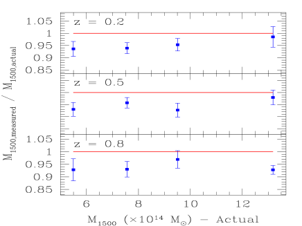
Figure 13: The ratio of the estimated mean mass to the true mass of the 10 simulated NFW clusters against the true masses. The errorbars are the standard deviation scaled by $1/\sqrt{10}$. The solid line is y = 1, depicting equality between the actual and measured masses.

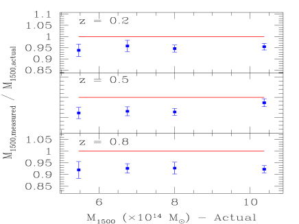
Figure 14: The ratio of the estimated mean mass to the true mass of the 10 simulated KKBP clusters, against the true masses. The errorbars are the standard deviation scaled by $1/\sqrt{10}$. The solid line is y = 1, depicting equality between the actual and measured masses.

The mass estimates for each of the clusters are summarized in Table 2 and Figures 12, 13 and 14. As mentioned earlier, these estimates correspond to the mass of the cluster at $1.5$ Mpc $\equiv M_{1500}$. Also, we assumed that the cluster profile was identified correctly; mass estimates for incorrectly identified clusters are discussed in the following section.

Table 2 shows that the cluster masses are correct to within a $10\%$ error at $M_{1500}\approx 0.5M_{\odot}$ that improves to $\leq 5\%$ at $M_{1500}\approx 1.5M_{\odot}$. The dependence of these estimates on redshift appears to be weak and there is no clear trend. This can possibly be attributed to the fact that although the physical extent of the images increases with increasing redshift, the signal falls off with increasing radial distance from the center of the cluster. This loss of signal with increasing redshift is also evident from an examination of the diagonal elements of Table 6.

An interesting feature of the data presented is the systematic $5\%$ bias in the mass estimates. Further numerical experiments pointed to the input ellipticity distribution as the cause of this bias. This dependence of the bias on the ellipticity distribution can be explained as follows: imagine we had assumed an ellipticity distribution of a $\delta$ function at zero ellipticity. In such a case, all mass estimates would be biased above since random elliptical galaxies would be erroneously interpreted as a weak lensing signal, indicating a mass distribution where none exists. Similarly, if we had assumed an intrinsic ellipticity distribution that had a greater fraction of elliptical galaxies than actually existed, such a distribution would result in an underestimate of the lensing and therefore the mass distribution.

It would appear, at first sight, that in our “experiments” we could avoid this by simply including our input ellipticity distribution, i.e. use Eq. 33 instead of Eq. 35. However, due to the finite size of galaxies and pixelization effects, the input ellipticity distribution and the observed ellipticity distribution are not the same. Our results correspond to estimates made with fits to the observed distribution, a choice further justified by the fact that any real observations must rely on such observed distributions since the true intrinsic distribution is unknown. This choice was borne out by numerical experiments that showed that estimates based on our Gaussian fit were more accurate than those from Eq. 33.

5.4 Mass Estimation - II

Table III: Mass Estimation - II - SIS clusters Redshift $M_{1500}(10^{15}M_{\odot})$ Profiles NFW KKBP z = 0.2 0.575 0.300 0.224 0.754 0.425 0.311 0.914 0.541 0.404 1.197 0.755 0.590 z = 0.5 0.575 0.382 0.285 0.754 0.522 0.405 0.914 0.640 0.525 1.197 0.906 0.780 z = 0.8 0.575 0.378 0.279 0.754 0.552 0.410 0.914 0.669 0.531 1.197 0.889 0.758 NFW KKBP

Table 3: The mean estimated masses for the SIS clusters when analyzed assuming an incorrect profile.

Table IV:Mass Estimation - II - NFW clusters Redshift $M_{1500}(10^{15}M_{\odot})$ Profiles SIS KKBP z = 0.2 0.550 0.717 0.331 0.756 1.012 0.488 0.951 1.253 0.636 1.318 1.722 0.991 z = 0.5 0.550 0.688 0.378 0.756 0.912 0.579 0.951 1.120 0.742 1.318 1.607 1.110 z = 0.8 0.550 0.673 0.394 0.756 0.872 0.552 0.951 1.111 0.755 1.318 1.565 1.096 SIS KKBP

Table 4: The mean estimated masses for the NFW clusters when analyzed assuming an incorrect profile.

Table V:Mass Estimation - II - KKBP clusters Redshift $M_{1500}(10^{15}M_{\odot})$ Profiles SIS NFW z = 0.2 0.546 0.943 0.734 0.675 1.166 0.943 0.800 1.364 1.135 1.037 1.738 1.347 z = 0.5 0.546 0.797 0.611 0.675 0.966 0.760 0.800 1.124 0.896 1.037 1.433 1.119 z = 0.8 0.546 0.766 0.582 0.675 0.942 0.735 0.800 1.087 0.860 1.037 1.331 1.080 SIS NFW

Table 5: The mean estimated masses for the KKBP clusters when analyzed assuming an incorrect profile.

Table VI: Average percentage bias Redshift Actual Bias SIS NFW KKBP z = 0.2 SIS -2.2 -40.5 -55.2 NFW 32.0 -4.2 -31.6 KKBP 70.3 38.3 -4.9 z = 0.5 SIS -3.1 -28.7 -41.6 NFW 19.5 -5.2 -20.8 KKBP 40.6 11.1 -6.1 z = 0.8 SIS -3.6 -26.5 -41.5 NFW 16.9 -5.1 -19.6 KKBP 34.9 7.0 -7.4 SIS NFW KKBP

Table 6: The observed percentage bias in $M_{1500}$ estimation for various assumed profiles.

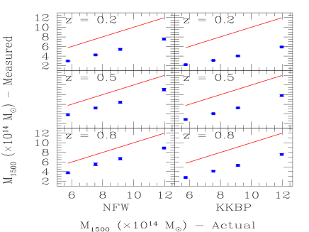
Figure 15: The estimated mean masses of the 10 simulated SIS clusters against the actual masses, if analyzed assuming an NFW or KKBP profile. The errorbars are the standard deviation scaled by $1/\sqrt{10}$. The solid line has slope $1$ and zero intercept, depicting equality between the actual and measured masses.

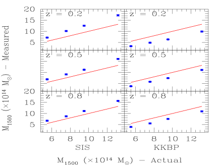
Figure 16: The estimated mean masses of the 10 simulated NFW clusters against the true masses, if analzyed assuming an SIS or KKBP profile. The errorbars are the standard deviation scaled by $1/\sqrt{10}$. The solid line has slope $1$ and zero intercept, depicting equality between the actual and measured masses.

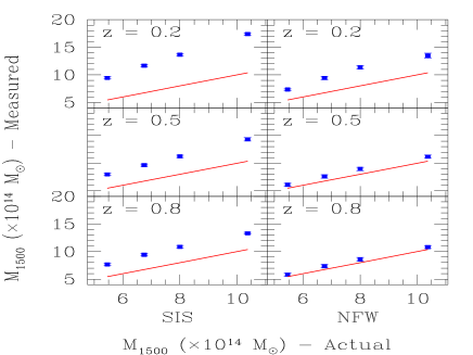
Figure 17: The estimated mean masses of the 10 simulated KKBP clusters against the true masses, if analzyed assuming an SIS or NFW profile. The errorbars are the standard deviation scaled by $1/\sqrt{10}$. The solid line has slope $1$ and zero intercept, depicting equality between the actual and measured masses.

The mass estimations discussed in the previous section assumed that the profile of the cluster was correctly identified. It is equally important to quantify the bias in the mass estimation if the incorrect profile is used, especially if we consider using these cluster masses for cosmology. Tables 3,4 and 5 and Figures 15, 16, and 17 summarize the mass estimation in our simulations when an incorrect profile is assumed. We also list the average bias as a function of redshift in Table 6. A clear trend is the reduction in the bias with increasing redshift; for instance the bias in KKBP clusters analysed as SIS clusters drops from 70% at $z=0.2$ to 35% at $z=0.8$, a reduction by a factor of two. This is easily explained by the fact that the degree of extrapolation decreases with increasing redshift since more of the cluster is visible and therefore the mass is better determined. Note also that the bias in an NFW/KKBP family cluster analysed with an SIS profile is of the order of 30% even at a redshift of 0.8, while the bias drops to 15% if the assumed profile was incorrect but part of the NFW/KKBP family. There is therefore a clear advantage to having some degree of profile determination before extrapolating.

5.5 Parameter Estimation

Table VII:$\delta_{c}$ / $\sigma_{v}$ Estimation Profile Type $\delta_{c}$ ($\times 10^{4}$) / Redshift $\sigma_{v}$ ($\times 10^{3}$ km/s) 0.2 0.5 0.8 SIS 0.913 0.886 0.887 0.887 1.045 1.016 1.023 1.029 1.150 1.140 1.116 1.128 1.317 1.310 1.319 1.302 NFW 1.57 1.59 1.68 1.72 2.15 2.28 1.92 2.12 2.70 2.80 3.19 2.45 3.75 3.68 3.63 4.35 KKBP 2.29 2.34 2.41 2.41 2.84 2.76 2.93 3.10 3.36 3.44 3.50 3.59 4.36 4.28 4.03 4.60 0.2 0.5 0.8

Table 7: The mean estimated values for $\delta_{c}$ ($\times 10^{4}$) for NFW and KKBP clusters and $\sigma_{v}$ ($\times 10^{3}$ km/s) for SIS clusters. The profiles are assumed to be correctly identified.

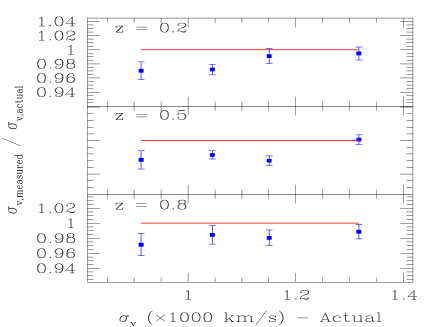
Figure 18: The ratio of the estimated $\sigma_{v}$ to the actual $\sigma_{v}$ of the 10 simulated SIS clusters plotted against the true values. The errorbars are the standard deviation scaled by $1/\sqrt{10}$. The solid line is y = 1, depicting equality between actual and measured $\sigma_{v}$.

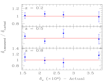
Figure 19: The ratio of the estimated $\delta_{c}$ to the actual $\delta_{c}$ of the 10 simulated NFW clusters plotted against the true values. The errorbars are the standard deviation scaled by $1/\sqrt{10}$. The solid line is y = 1, depicting equality between actual and measured $\delta_{c}$.

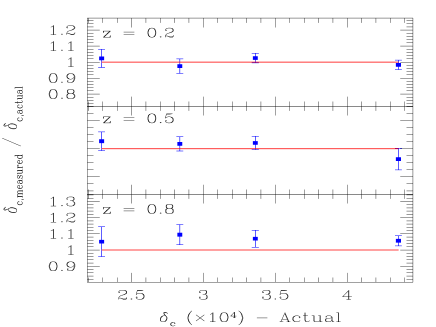
Figure 20: The ratio of the estimated $\delta_{c}$ to the actual $\delta_{c}$ of the 10 simulated KKBP clusters plotted against the true values. The errorbars are the standard deviation scaled by $1/\sqrt{10}$. The solid line is y = 1, depicting equality between actual and measured $\delta_{c}$.

Table VIII:$\theta_{s}$ Estimation Profile Type $\theta_{s,true}$ Mass ($10^{15}M_{\odot}$) (arcsec) 0.5 0.75 1.0 1.5 SIS 4.3 3.5 3.6 5.1 5.1 2.3 2.3 2.1 1.5 4.0 1.9 1.9 2.5 2.4 2.7 NFW 86.6 85.7 83.5 86.0 97.7 46.8 45.0 50.2 45.0 54.0 38.0 37.5 38.7 44.2 36.2 KKBP 64.5 62.7 64.5 62.5 64.0 34.9 33.5 33.7 33.5 36.5 28.3 27.5 26.7 27.0 27.0 0.5 0.75 1.0 1.5

Table 8: The mean estimated values for $\theta_{s}$ in arcseconds. The profiles are assumed to be correctly identified.

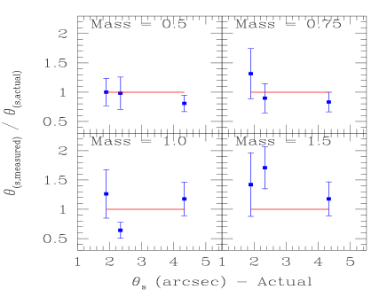
Figure 21: The ratio of the estimated $\theta_{s}$ to the actual $\theta_{s}$ of the 10 simulated SIS clusters plotted against the true values. The errorbars are the standard deviation scaled by $1/\sqrt{10}$. The solid line is y = 1, depicting equality between actual and measured $\theta_{s}$.

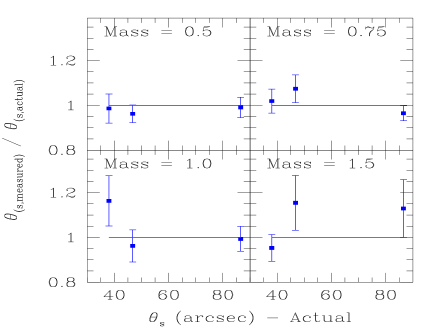
Figure 22: The ratio of the estimated $\theta_{s}$ to the actual $\theta_{s}$ of the 10 simulated NFW clusters plotted against the true values. The errorbars are the standard deviation scaled by $1/\sqrt{10}$. The solid line is y = 1, depicting equality between actual and measured $\theta_{s}$.

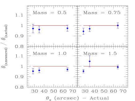
Figure 23: The ratio of the estimated $\theta_{s}$ to the actual $\theta_{s}$ of the 10 simulated KKBP clusters plotted against the true values. The errorbars are the standard deviation scaled by $1/\sqrt{10}$. The solid line is y = 1, depicting equality between actual and measured $\theta_{s}$.

The parameter estimates for our simulations are summarized in Tables 7 and 8 and Figures 18 to 23. The most striking feature about these data is that the parameters are estimated to within $25\%$ even though the masses were estimated with a $\leq 10\%$ error. This is explained by realizing that there is a degeneracy in determining the parameters for a given mass, increasing the variance in the parameter estimation. However, the correlated errors in the parameters combine to give a smaller cumulative error in the mass.

It is also relevant to note that the errors in the estimation of the core radius for SIS clusters are significantly greater than the corresponding errors in the scale radius for NFW/KKBP clusters. This is a result of the fact that the core radius for the SIS clusters is $\approx 10$ kpc and therefore has little effect on the observed weak lensing. On the other hand, the scale radius in the NFW/KKBP clusters affects the mass profile of the cluster at significantly greater scales and is therefore probed by weak lensing. Any attempt to robustly estimate the core radius for SIS clusters must rely on strong lensing.

6 Discussion

We have studied the reliability of mass profile determinations for clusters of galaxies using a parametric inversion method. We found that the mass profiles of different “families” of profiles could be reliably determined to within $80$%. We appear to able to distinguish profiles motivated by N-body CDM simulations (in our case, NFW and KKBP) from the canonical $r^{-2}$ SIS profile, making our method a promising approach to test this prediction. However, we were unable to distinguish between the various “flavours” of models predicted by N-body simulations since these models only differ in their inner cores and are therefore inaccessible to weak lensing. Strong lensing analyses of arcs, sensitive to this inner core might prove to be sufficient to constrain the inner parts of the profiles but this still remains an open question.

We also examined the biases in mass estimates when an incorrect cluster profile (eg. SIS) is assumed and found that these biases can be quite significant ($\sim 70$%), especially at low redshifts ($z\sim 0.2$). At higher redshifts, the bias is weaker, although still substantial at $\sim 50$%. This redshift dependence was traced to the fact that at higher redshifts, images of a given angular extent correspond to a greater physical extent. Weak lensing constrains the mass within the observed area, but in order to estimate the virial mass (or $M_{1500}$), one must extrapolate to the appropriate radius. Using an incorrect profile for this extrapolation will bias the mass estimate. However, the degree of extrapolation decreases with increasing redshift, reducing the bias.

Finally, we also showed that the method could extract the correct cluster profile parameters although only to within $25$%. The greater errors in this case can be traced to a degeneracy in the parameters for a given mass; such a degeneracy would naturally broaden the likelihood function and increase the errors. The case for a degeneracy is further strengthed by the fact that the mass estimates are significantly more robust, being within $10$%.

This paper represents a first attempt to demonstrate the feasibility of our method and estimate the reliability of profile determination and the bias introduced in the mass estimate due to an incorrect profile. For simplicity, we have left a number of practical aspects unaddressed which we now consider. The most relevant issue is the measurement of the intrinsic ellipticity distribution. We computed this distribution self consistently in our simulation. A real world application must determine this background ellipticity distribution in fields away from significant weak lensing sources. The Medium Deep Survey (Ratnatunga et. al 1999) is one such possibility. There are a number of concerns with this approach such as the evolution of the ellipticity distribution with redshift and the effects of the instrument of the ellipticity distribution, that still remain unexplored.

A second area that must be incorporated into the method is the redshift distribution of the lensed galaxies, since the strength of the lensing is dependent on the distance between the galaxy and the lens. There are two possible approaches to solving this problem within the framework of our method. The first is to use photometric redshifts and use those as a second input parameter in Eq. 38

$${\cal L}=-\sum_{i=1}^{N}\log p(\mbox{\boldmath$\epsilon$}_{i},z_{i};\delta_{i},\theta_{i})\,.$$ (37)

The second is to convolve a redshift distribution directly into the likelihood function and measure its parameters from the data itself. Eq. 38 would then read

$${\cal L}=-\sum_{i=1}^{N}\log p(\mbox{\boldmath$\epsilon$}_{i};\delta_{i},\theta_{i},\bf{z_{i}})\,.$$ (38)

where $\bf{z_{i}}$ represents the parameters of the redshift distribution. The generic effect of such an approach would be to broaden the likelihood function and therefore, increase the errors in the measurements.

Finally, the effect of seeing on these results must be addressed. Seeing, as it tends to circularise images, would generically reduce the lensing signal and therefore result in an underestimate of the mass distribution. The measured intrinsic ellipticity distribution would also be affected by seeing, and this may compensate for the effects of seeing, although a definitive answer must wait for further simulations that include seeing.

In spite of as yet unexplored observational effects relevant to our technique, our formalism still calls for an observational test of theoretical predictions of cluster profiles. Improvements in telescopes designs for weak lensing searches ought to make this a feasible approach in the future.

Appendix A Analytic forms of the Convergence and Shear for Specific Models

The convergence and shear for a circularly symmetric mass distribution were given by equations 14 and 19 in the main text . In this Appendix we derive specific expressions for the SIS, NFW, and KKPB cluster profiles.

A.1 SIS

The density law for a softened isothermal sphere with a core radius $r_{s}$ is

$$\rho(r)=\frac{\sigma_{v}^{2}}{2\pi Gr_{s}^{2}}\left[\frac{1}{1+\left(r/r_{s}\right)^{2}}\right]\,.$$ (39)

Making the connection with the formalism developed in § 2, $\eta(x)=(1+x^{2})^{-1}$ and $\delta_{c}=4\sigma_{v}^{2}/3(H_{0}r_{s})^{2}.$ This form of $\eta(x)$ leads straightforwardly to the following expressions for $\beta(x)$ and its derivative:

$$\beta(x)=\frac{\pi}{2}\left(\sqrt{x^{2}+1}-1\right)$$ (40)

$$\beta^{\prime}(x)=\frac{\pi}{2}\frac{x}{\sqrt{1+x^{2}}}\,,$$ (41)

and thus yields the convergence and shear for the SIS model:

$$\kappa(x)=\frac{2\pi\sigma_{v}^{2}}{c^{2}}\,\theta_{s}^{-1}\frac{y_{LS}}{y_{S}}\frac{1}{\sqrt{1+x^{2}}}\,,$$ (42)

$$\gamma(x)=\frac{2\pi\sigma_{v}^{2}}{c^{2}}\,\theta_{s}^{-1}\frac{y_{LS}}{y_{S}}\left(\frac{1}{\sqrt{1+x^{2}}}-\frac{2}{1+\sqrt{1+x^{2}}}\right)\,,$$ (43)

where $x=\theta/\theta_{s}$ and $\theta_{s}=r_{s}/D_{L}.$

A.2 NFW

For NFW we have $\eta(x)=x^{-1}(1+x)^{-2},$ and thus

$$\beta(x)=\int_{0}^{x}y\,dy\int_{0}^{\infty}\frac{dw}{\sqrt{y^{2}+w^{2}}\left(1+\sqrt{y^{2}+w^{2}}\right)^{2}}\,.$$ (44)

Making the change of variable $\tan\theta=w/y,$ we obtain

$$\beta(x)=\int_{0}^{x}y\,dy\int_{0}^{\pi/2}\frac{\cos\theta\,d\theta}{\left(y+\cos\theta\right)^{2}}\,.$$ (45)

We now change the order of integration, and the $y$-integral is readily done, yielding

$$\beta(x)=\int_{0}^{\pi/2}\cos\theta\ln\left[1+\frac{x}{\cos\theta}\right]\,d\theta$$

$$+\int_{0}^{\pi/2}\frac{\cos^{2}\theta\,d\theta}{x+\cos\theta}\,-1\,.$$

We now write $\ln(1+x/\cos\theta)=\ln(\cos\theta+x)-\ln(\cos\theta),$ integrate the first term by parts, and then obtain after some manipulation

$$\beta(x)=\ln x+\int_{0}^{\pi/2}\frac{d\theta}{\cos\theta+x}$$

$$+\int_{0}^{\pi/2}\cos\theta\,\ln(\sec\theta)\,d\theta-1\,.$$

The second integral above has the value $1-\ln 2$ (Gradshteyn & Ryzhik 1994, Eq. 4.387). Thus,

$$\beta(x)=\ln(x/2)+{\cal F}(x)\,,$$ (46)

where

$${\cal F}(x)\equiv\int_{0}^{\pi/2}\frac{d\theta}{\cos\theta+x}\,,$$ (47)

and has the following values (Gradshteyn & Ryzhik 1994, Eq. 2.553):

1. $x<1$:

   $${\cal F}(x)=\frac{1}{\sqrt{1-x^{2}}}\,\ln\left(\frac{x}{1-\sqrt{1-x^{2}}}\right)$$ (48)

2. $x>1$:

   $${\cal F}(x)=\frac{1}{\sqrt{x^{2}-1}}\,\cos^{-1}(1/x)$$ (49)

3. $x=1$:

   $${\cal F}(x)=1$$ (50)

Differentiating equation 46 yields

$$\beta^{\prime}(x)=\frac{1}{x}+{\cal F}^{\prime}(x)$$ (51)

where

$${\cal F}^{\prime}(x)=-\int_{0}^{\pi/2}\frac{d\theta}{(x+\cos\theta)^{2}}\,.$$ (52)

Carrying out the integral (Gradshteyn & Ryzhik 1994, Eq. 2.553) then leads to

$${\cal F}^{\prime}(x)=\frac{1}{x^{2}-1}\left[\frac{1}{x}-x{\cal F}(x)\right]$$ (53)

and

$${\cal F}^{\prime}(1)=-\frac{2}{3}\,.$$ (54)

Equations A10–A18 above enable use to calculate bending angle, convergence, and shear for an NFW model of specified $\delta_{c}$ and $\theta_{s},$ by means of equations 10, 14, and 19 of the main text.

A.3 KKBP

A KKBP halo has $\eta(x)=x^{-0.2}(1+x^{2})^{-1.4},$ and thus

$$\beta(x)=\int_{0}^{x}y\,\sigma(y)\,dy\,,$$ (55)

where

$$\sigma(y)=\int_{0}^{\infty}(y^{2}+w^{2})^{-0.1}[1+y^{2}+w^{2}]^{-1.4}dw\,.$$ (56)

Unlike the SIS and NFW halos, there is no analytical form for the functions $\beta$ and $\sigma$ for KKBP. We have therefore integrated equation 56 numerically, and fit the results to a rational function. The following expression provides a fit accurate to better than 1%:

$$\sigma(x)=\frac{1.250+0.965133x}{1+1.18363x+1.06347x^{2}+x^{3}}\,.$$ (57)

Substitution of this expression into equation 55 allows one to obtain an analytic expression for $\beta(x)$ via integration:

$$\beta(x)=-0.0558209+\beta_{1}(x)+\beta_{2}(x)+\beta_{3}(x)\,,$$ (58)

where:

$$\beta_{1}(x)=0.126086\tan^{-1}(0.0605662+0.970072x)$$ (59)

$$\beta_{2}(x)=-0.176946\ln(0.937601+x)$$ (60)

$$\beta_{3}(x)=0.571039\ln(1.06655+0.124869x+x^{2})\,.$$ (61)

Appendix B Determination of Cluster Virial Masses

The virial mass of a cluster, $M_{V},$ is defined to be the mass within a sphere whose mean interior density is larger than the background density by a particular factor. The radius of the sphere is called the virial radius, $R_{V}.$ In an Einstein-de Sitter universe the factor is $178$; in open and flat low-density universes the factor is larger. For the purposes of this paper, we simply assume the factor is known, and denote it $\delta_{V}.$ (In the main body of the paper we take $\delta_{V}=200.$) In this Appendix we show how to calculate $M_{V}$ and $R_{V}$ for a given density law.

As usual, we write the halo density profile as $\rho(r)=\rho_{crit}\delta_{c}\eta(x),$ where $x=r/r_{s}$ and $r_{s}$ is the characteristic radius. The mass interior to a radius $R$ is thus

$$M(R)=4\pi r_{s}^{3}\rho_{crit}\delta_{c}m(y)\,,$$ (62)

where $y=R/r_{s}$ and $m(y)$ is the dimensionless mass profile given by

$$m(y)=\int_{0}^{y}x^{2}\eta(x)dx\,.$$ (63)

The condition that the mean density within $R_{V}$ is $\delta_{V}$ times the background density is

$$\frac{M(r_{V})}{4\pi r_{V}^{3}/3}=\delta_{V}\Omega_{M}\rho_{crit}\,.$$ (64)

Combining this with equation 62 yields

$$m(y_{V})=\frac{\delta_{V}}{3\delta_{c}}\Omega_{M}y_{V}^{3}\,,$$ (65)

where $y_{V}\equiv R_{V}/r_{s}.$ For any given density law $\rho(r)$ and value of $\Omega_{M},$ equation 65 can be solved for $y_{V},$ which in turn yields the virial radius $R_{V}=y_{V}r_{s},$ and the virial mass through equation 62.

The integral in equation 63 is readily carried out for the SIS and NFW density profiles, yielding

$$m_{SIS}(y)=y-\tan^{-1}y$$ (66)

and

$$m_{NFW}(y)=\ln(1+y)-\frac{y}{1+y}\,.$$ (67)

It is useful to express the virial mass in terms of typical halo parameters. From equation 62 one finds:

$$M_{V}=3.49\times 10^{14}\left(\frac{r_{s}}{100\ {\rm kpc}}\right)^{3}\left(\frac{\delta_{c}}{10^{5}}\right)m(y_{V})\,h^{-1}M_{\odot}\,.$$ (68)

For example, a KKBP halo with for $r_{s}=100$ kpc and $\delta_{c}=10^{5}$ has $M_{V}=8.7\times 10^{14}\,h^{-1}M_{\odot},$ and $r_{V}=1.55$ Mpc, for $\delta_{V}=200.$

References

- [] Bahcall, N.A. 2000, Phys. Scripta, T85, 32, (astro-ph/9901076)
- [] Bahcall, N.A., & Cen, R. 1993, ApJL, 407, L49
- [] Bahcall, N.A., Fan, X., Cen, R. 1997, ApJL, 485, L53
- [] Bartelmann, M., & Schneider, P. 1999, preprint (astro-ph/9912508)
- [] Bartelmann, M. 1998, Evolution of Large-Scale Structure: From Recombination to Garching, E28
- [] Bartelmann, M. 1996, 313, 697
- [Blanchard, Sadat, Bartlett & Le Dour(2000)] Blanchard, A., Sadat, R., Bartlett, J. & Le Dour, M. 2000, ASP Conf. Ser. 200: Clustering at High Redshift, 158 (astro-ph/9908037)
- [Borgani, Rosati, Tozzi & Norman(1999)] Borgani, S., Rosati, P., Tozzi, P. & Norman, C. 1999, ApJ, 517, 40 (astro-ph/9901017)
- [] Carlberg, R. G. et al. 1998, Large Scale Structure: Tracks and Traces, 119
- [] Carlberg, R. G., Morris, S. L., Yee, H. K. C. & Ellingson, E. 1997, ApjL, 479, L19
- [Donahue et al.(1998)] Donahue, M., Voit, G. M., Gioia, I., Lupino, G., Hughes, J. P. & Stocke, J. T. 1998, ApJ, 502, 550
- [Eke, Cole, Frenk & Patrick Henry(1998)] Eke, V. R., Cole, S., Frenk, C. S. & Patrick Henry, J. 1998, MNRAS, 298, 1145
- [Girardi et al.(1998)] Girardi, M., Borgani, S., Giuricin, G., Mardirossian, F. & Mezzetti, M. 1998, ApJ, 506, 45
- [Gradshteyn & Ryzhik(1994)] Gradshteyn, I. S. & Ryzhik, I. M. 1994, New York: Academic Press
- [] Hoekstra, H., Franx, M., Kuijken, K., & Squires, G. 1998, ApJ, 504, 636
- [] Kaiser, N., & Squires, G. 1993, ApJ, 404,441
- [Kaiser, Tonry & Luppino(2000)] Kaiser, N., Tonry, J. L. & Luppino, G. A. 2000, PASP, 112, 76 (astro-ph/9912181)
- [] Kravtsov, A.V., Klypin, A.A., Bullock, J.S., & Primack, J.R. 1998, ApJ, 502, 48 (KKBP)
- [Lewis, Ellingson, Morris & Carlberg(1999)] Lewis, A. D., Ellingson, E., Morris, S. L. & Carlberg, R. G. 1999, ApJ, 517, 587 (astro-ph/9901062)
- [] Lewis, A.D., Ellingson, E., Morris, S.L., & Carlberg, R.G. 1999, preprint (astro-ph/9901062)
- [Lewis, Ellingson, Morris & Carlberg(1999)] Lewis, A. D., Ellingson, E., Morris, S. L. & Carlberg, R. G. 1999, ApJ, 517, 587
- [] Luppino, G.A., & Kaiser, N. 1997, ApJ, 475, 20
- [] Luppino, G.A., Tonry, J.L., & Stubbs, C.W. 1998, Proc. SPIE, 3355, 469
- [Miralda-Escude(1991)] Miralda-Escude, J. 1991, ApJ, 370, 1 (ME91)
- [] Navarro, J.F., Frenk, C.S., & White, S.D.M. 1997, ApJ, 490, 493 (NFW)
- [] Narayan, R., & Bartelmann, M. 1999, in Formation of Structure in the Universe, eds. A. Dekel & J.P. Ostriker (Cambridge University Press) (NB99)
- [Peebles(1993)] Peebles, P. J. E. 1993, Princeton Series in Physics, Princeton, NJ: Princeton University Press
- [Ratnatunga, Griffiths & Ostrander(1999)] Ratnatunga, K. U., Griffiths, R. E. & Ostrander, E. J. 1999, AJ, 118, 86
- [Reichart et al.(1999)] Reichart, D. E., Nichol, R. C., Castander, F. J., Burke, D. J., Romer, A. K., Holden, B. P., Collins, C. A. & Ulmer, M. P. 1999, ApJ, 518, 521 (astro-ph/9802355)
- [Sadat, Blanchard & Oukbir(1998)] Sadat, R., Blanchard, A. & Oukbir, J. 1998, A&A, 329, 21
- [] Schneider, P., & Seitz, C. 1995, A&A, 294, 411
- [] Seitz, C., & Schneider, P. 1995, A&A, 297, 287
- [] Seitz, C., & Schneider, P. 1996, A&A, 305, 383
- [] Seitz, C., & Schneider, P. 1997, A&A, 318, 687
- [] Seitz, C., Schneider, P., & Bartelmann, M. 1998, A&A, 337, 325
- [Smail et al.(1997)] Smail, I., Ellis, R. S., Dressler, A., Couch, W. J., Oemler, A. J., Sharples, R. M. & Butcher, H. 1997, ApJ, 479, 70
- [Squires & Kaiser(1996)] Squires, G. & Kaiser, N. 1996, ApJ, 473, 65
- [Squires et al.(1997)] Squires, G., Neumann, D. M., Kaiser, N., Arnaud, M., Babul, A., Boehringer, H., Fahlman, G. & Woods, D. 1997, ApJ, 482, 648
- [] Tran, K.-V. H., Kelson, D.D., van Dokkum, P., Franx, M., Illingworth, G.D., & Magee, D. 1999, ApJ, 522, 39
- [Tyson & Seitzer(1988)] Tyson, J. A. & Seitzer, P. 1988, ApJ, 335, 552
- [Tyson(1988)] Tyson, J. A. 1988, AJ, 96, 1
- [] Tyson, J.A., Kochanski, G.P., & Dell’Antonio, I.P. 1998, ApJ, 498, L107
- [Tyson, Wenk & Valdes(1990)] Tyson, J. A., Wenk, R. A. & Valdes, F. 1990, ApJL, 349, L1
- [] Valdes, F., 1982, Faint Object Classification and Analysis System, NOAO document
- [van den Bosch & Swaters(2000)] van den Bosch, F. C. & Swaters, R. A. 2000, Submitted for publication in AJ (astro-ph/0006048)
- [White, Efstathiou & Frenk(1993)] White, S. D. M., Efstathiou, G. & Frenk, C. S. 1993, MNRAS, 262, 1023
- [Willick(2000)] Willick, J. A. 2000, ApJ, 530, 80
- [Wilson, Cole & Frenk(1996)] Wilson, G., Cole, S. & Frenk, C. S. 1996, MNRAS, 280, 199
- [] Wu, X.P., Chiueh, T., Fang, L.Z., & Xue, Y.J. 1998, MNRAS, 301, 861