How to measure CMB polarization power spectra without losing information

Abstract

We present a method for measuring CMB polarization power spectra given incomplete sky coverage and test it with simulated examples such as Boomerang 2001 and MAP. By augmenting the quadratic estimator method with an additional step, we find that the $E$ and $B$ power spectra can be effectively disentangled on angular scales substantially smaller than the width of the sky patch in the narrowest direction. We find that the basic quadratic and maximum-likelihood methods display a unneccesary sensitivity to systematic errors when $T-E$ cross-correlation is involved, and show how this problem can be eliminated at negligible cost in increased error bars. We also test numerically the widely used approximation that sample variance scales inversely with sky coverage, and find it to be an excellent approximation on scales substantially smaller than the sky patch.

]

I Introduction

As experimental groups roar ahead to map the CMB intensity with increasing resolution and sensitivity, a second parallel front is being opened up: CMB polarization. Theoretical advances now allow model predictions for CMB polarization to be computed with exquisite accuracy [1, 2, 3], and it is known that polarization measurements can substantially improve the accuracy with which parameters can be measured over the no-polarization case by breaking the degeneracy between certain parameter combinations [4, 5, 6]. CMB polarization can also provide crucial cross-checks and tests of the underlying theory. After placing ever tighter upper limits [7, 8], a number of experimental teams are likely to make the first detections of CMB polarization in the next year or two, about a decade after unpolarized CMB fluctuations were first detected [9]. It is therefore timely to address real-world issues related to extracting polarized power spectra from experiments with incomplete sky coverage and complicated noise. This is the purpose of the present paper, with emphasis on the problem of separating the two polarization signals known as $E$ and $B$ [1, 2]. Important steps in this direction were first taken in [10, 11], for the special case of experiments mapping circles in the sky.

The $E/B$ problem goes back to the fact that the polarization tensor field on the sky can be separated into a curl-free and a divergence free component, and is most naturally expressed in terms of two scalar fields, denoted $E$ and $B$ by analogy with electromagnetism [1, 2]. Not only does this separation eliminate the coordinate system dependence that plagues the familiar Stokes parameters, but $E$ and $B$ also probe distinct physical effects, making them the natural meeting point for theory and observation. Unfortunately, the correspondence between $E$ and $B$ and the measured Stokes parameters is not spatially local, involving a partial differential equation, which means that it is not possible to uniquely recover $E$ and $B$ from a map with merely partial sky coverage. This issue is particularly important since the $B$-signal from inflation-produced gravity waves potentially offers a unique probe of ultra-high-energy physics, but may be swamped by a leakage from a larger $E$-signal [12, 13].

A key goal of CMB analysis is to constrain cosmological models, and information-theoretical methods have been frequently employed in the literature to study how accurately this can be done in principle with a given data set, using the Fisher information matrix formalism [14, 15]. For CMB polarization experiments, this has been useful both for optimizing experimental design [16, 17] and for accuracy forecasting in general [4]. These information-theoretical tools are equally useful for data analysis, since they provide a simple way of checking whether cosmological information is being lost in the data analysis pipeline. Each step in such a pipeline typically compresses the input data into a smaller set of numbers, and if the output can be shown to retain all the cosmological information of the input, the method is said to be lossless. Lossless methods have been developed and extensively tested for the unpolarized case, for both mapmaking [18, 19] and power spectrum estimation [20, 21]. As we will see, it is possible to draw heavily on these methods for the polarized case as well, although a number of adaptations make them simpler to interpret and help improve the $E/B$-separation and robustness towards systematic errors.

The rest of this paper is organized as follows. In Section II, we discuss basic methods involved in polarization data analysis. To keep the presentation from becoming too abstract, many method details and extensions are postponed to Section III, where they are illustrated with plots from actual applications. This section also assesses the effectiveness of the various methods numerically, with applications to five experimental examples. A step-by-step summary of how to compute the signal covariance matrix is given in Appendix A for the reader wishing to do so in practice. Our conclusions are summarized in Section IV.

II Method

In this section, we first establish some basic notation, then discuss the extraction of maps from raw time-ordered data, and finally cover the extraction of power spectra from maps.

A Notation

The linear polarization pattern of the CMB sky is characterized by the two Stokes parameters $Q$ and $U$ in each sky direction. $Q$ and $U$ are the components of a rank 2 tensor (spinor), loosely speaking a vector without an arrow on it, so $Q$ and $U$ maps are defined only relative to a convention providing a reference direction at each point in the sky. Let us discretize the $T$, $Q$ and $U$ maps into $N$ pixels centered at unit vectors $\widehat{\bf r}_{1},...,\widehat{\bf r}_{N}$, and write $T_{i}=T(\widehat{\bf r}_{i})$, $Q_{i}=Q(\widehat{\bf r}_{i})$, $U_{i}=U(\widehat{\bf r}_{i})$ (we let $T$ denote the unpolarized intensity, often called $I$). We group these numbers into three $N$-dimensional vectors ${\bf T}$, ${\bf Q}$ and ${\bf U}$ and group these in turn into a single $3N$-dimensional vector

$${\bf x}\equiv\left(\begin{tabular}[]{c}${\bf T}$\\ ${\bf Q}$\\ ${\bf U}$\end{tabular}\right).$$ (1)

The statistical properties of ${\bf x}$ have been computed in full detail in the literature [1, 2], and are characterized by six separate power spectra: $C_{\l}^{T}$ for the unpolarized signal $T$, $C_{\l}^{E}$ for the $E$-polarization, $C_{\l}^{B}$ for the $B$-polarization, and $C_{\l}^{TE}$, $C_{\l}^{TB}$ and $C_{\l}^{EB}$ for the three possible cross-correlations. The power spectra $C_{\l}^{TB}$ and $C_{\l}^{EB}$ are both predicted to vanish for the CMB, but it will be interesting to measure them nonetheless, as probes of polarized foregrounds and exotic parity-violating physics [51]. We will occasionally refer to the three cross-correlations $(TE,TB,EB)$ as $(X,Y,Z)$, respectively. We will find it useful for data analysis purposes to recast the polarization problem in exactly the same mathematical form as the simpler unpolarized case, encoding all complications in a set of matrices. The vector ${\bf x}$ has a vanishing expectation value (${\langle{\bf x}\rangle={\bf 0}}$), and we can write its covariance matrix as

$${\bf C}\equiv\langle{\bf x}{\bf x}^{t}\rangle=\sum_{i}p_{i}{\bf P}_{i}$$ (2)

for a set of parameters $p_{i}$ and known matrices ${\bf P}_{i}$. If the six observed power spectra are negligibly small for all multipoles $\l$ above some value ${\ell_{\rm max}}$ (which is always the case because of the smoothing caused by the finite angular resolution of an experiment), then we define these parameters to be

$$\cases{p_{1},...,p_{{\ell_{\rm max}}-1}&$={\delta T^{2}}^{T}_{2},..{\delta T^{2}}^{T}_{\ell_{\rm max}}$,\cr\vskip 4.0pt\cr p_{{\ell_{\rm max}}},...,p_{2{\ell_{\rm max}}-2}&$={\delta T^{2}}^{E}_{2},..{\delta T^{2}}^{E}_{\ell_{\rm max}}$,\cr\vskip 4.0pt\cr p_{2{\ell_{\rm max}}-1},...,p_{3{\ell_{\rm max}}-3}&$={\delta T^{2}}^{B}_{2},..{\delta T^{2}}^{B}_{\ell_{\rm max}}$,\cr\vskip 4.0pt\cr p_{3{\ell_{\rm max}}-2},...,p_{4{\ell_{\rm max}}-4}&$={\delta T^{2}}^{TE}_{2},..{\delta T^{2}}^{TE}_{\ell_{\rm max}}$,\cr\vskip 4.0pt\cr p_{4{\ell_{\rm max}}-3},...,p_{5{\ell_{\rm max}}-5}&$={\delta T^{2}}^{TB}_{2},..{\delta T^{2}}^{TB}_{\ell_{\rm max}}$,\cr\vskip 4.0pt\cr p_{5{\ell_{\rm max}}-4},...,p_{6{\ell_{\rm max}}-6}&$={\delta T^{2}}^{EB}_{2},..{\delta T^{2}}^{EB}_{\ell_{\rm max}}$,\cr\vskip 4.0pt\cr p_{6{\ell_{\rm max}}-5}&$=\eta=1.$}$$ (3)

Here

$${\delta T^{2}}_{\l}^{P}\equiv{\l(\l+1)\over 2\pi}C^{P}_{\l}$$ (4)

is the familiar rescaled power that is normally used in power spectrum plots in place of $C^{P}_{\l}$. The index $P$ denotes any of the six power spectrum types, i.e., $P=T,E,B,TE,TB,EB$. The parameter $\eta$ is the normalization of the detector noise in the maps relative to the predicted value, and is normally equal to unity. Since ${\bf C}$ depends linearly on the parameters $p_{i}$, we can define the ${\bf P}$-matrices as

$${\bf P}_{i}\equiv{\partial{\bf C}\over\partial p_{i}}.$$ (5)

In other words, the first $6({\ell_{\rm max}}-1)$ ${\bf P}$-matrices give the contributions from the $T$, $E$, $B$, $TE$, $TB$ and $EB$ power spectra, and the last one is simply the noise covariance matrix, giving the contribution from experimental noise.

Appendix A summarizes how to compute the ${\bf C}$-matrix, and is intended for the reader who wishes to write software to do this in practice. The ${\bf P}$-matrix corresponding to ${\delta T^{2}}_{\l}^{P}$ is obtained from these formulas by simply setting all power spectra to zero, with the single exception ${\delta T^{2}}_{\l}^{P}=1$, i.e., $C^{P}_{\l}=2\pi/\l(\l+1)$. These ${\bf P}$-matrices are therefore independent of the actual power spectra, and depend merely on the relative orientations of the map pixels.

B Background: from timestream to $T$, $Q$ & $U$ maps

To place our problem in context, this section briefly reviews how to reduce experimental data to maps in the form of equation (1). Although it is widely known how to do this, we will see that there are some subtle issues related to unmeasured modes.

1 The basic inversion

Suppose we have observed the sky a large number of times with (perhaps) polarized detectors in a variety of different orientations. Let $y_{i}$ denote the number measured in the $i^{th}$ observation, and group this time-ordered data set (TOD) into an $M$-dimensional vector ${\bf y}$. The observed temperature fluctuation $y_{i}$ seen through a linear polarizer takes the form

$$y_{i}={1\over 2}\left[T_{k_{i}}+Q_{k_{i}}\cos(2\alpha_{i})+U_{k_{i}}\sin(2\alpha_{i})\right]+n_{i},$$ (6)

where $\alpha_{i}$ gives the clockwise angle between the polarizer and the reference direction of the coordinate system, $n_{i}$ denotes the detector noise, and $k_{i}$ is the number of the pixel pointed to during the $i^{th}$ observation. If the experiment instead measures the difference between two perpendicular polarizations, $y_{i}$ takes the simpler form

$$y_{i}=Q_{k_{i}}\cos(2\alpha_{i})+U_{k_{i}}\sin(2\alpha_{i})+n_{i},$$ (7)

An unpolarized experiment is described by $y_{i}=T_{k_{i}}+n_{i}$. Grouping the numbers into vectors, we can write any of these three expressions as a simple matrix equation

$${\bf y}={\bf A}{\bf x}+{\bf n},$$ (8)

where the matrix ${\bf A}$ encompasses all the relevant details of the observations. For a pure polarization experiment as in equation (7), ${\bf A}$ will contain only zeroes except for a single sine and cosine entry in each row, in columns corresponding to the pixel observed. More general observing strategies such as the beam-differencing of the MAP Satellite or modulated beams clearly retain the simple form of equation (8), merely with a slightly more complicated (but known) ${\bf A}$-matrix. For a well-designed experiment such as MAP, the system of equations (8) is highly overdetermined, and the estimate $\tilde{\bf x}$ of the map triplet ${\bf x}$ given by the familiar equation [18]

$$\tilde{\bf x}={\bf W}{\bf y},\quad{\bf W}\equiv[{\bf A}^{t}{\bf M}{\bf A}]^{-1}{\bf A}^{t}{\bf M}$$ (9)

is unbiased ($\langle\tilde{\bf x}\rangle={\bf W}{\bf A}{\bf x}+{\bf W}\langle{\bf n}\rangle={\bf x}$ since ${\bf W}{\bf A}={\bf I}$). If ${\bf M}$ a reasonable approximation to ${\bf N}^{-1}$, then the map noise ${\bf W}{\bf n}$ will have minimum variance to first order, with covariance matrix ${\bf\Sigma}\equiv{\bf W}{\bf N}{\bf W}^{t}\approx[{\bf A}^{t}{\bf N}^{-1}{\bf A}]^{-1}$. Both the map triplet $\tilde{\bf x}$ and its exact noise covariance matrix ${\bf\Sigma}$ can be computed in $\sim N^{3}$ time, and even faster in many important cases [19, 22, 23, 24, 25, 26, 27, 28, 29, 30]. Note that the last ${\bf P}$-matrix is this noise covariance matrix, i.e., ${\bf P}_{6{\ell_{\rm max}}-5}={\bf\Sigma}$.

2 The problem of missing modes

In many cases, the inversion in equation (9) fails because the matrix to be inverted is singular. Although there are typically much more measurements $y_{i}$ than unknowns $x_{i}$ ($M\gg 3N$), symmetries or other properties of the observing strategy often imply that ${\bf A}^{t}{\bf x}={\bf 0}$ for certain vectors ${\bf x}$, i.e., that ${\bf A}$ is singular. A ubiquitous example is lack of sensitivity to the mean (monopole) in the map. Experiments measuring linear polarization without cross-linking may be sensitive to only a certain linear combination of $Q$ and $U$, unable to recover the two separately. As another example, the PIQUE experiment [7] measures only sums of $Q$-values $90^{\circ}$ apart on a circle in the sky, thereby losing information about modes taking values $(+1,-1,+1,-1)$ at four corners of a square.

All such problems can in principle be dealt with by regularizing the inversion (see, e.g., the Appendix of [20]), which sets the unmeasurable modes to zero in the final maps, and keeping track of which modes are missing during subsequent analysis of $\tilde{\bf x}$. In practice, however, it is often more convenient to eliminate this extra bookkeeping requirement by encoding the corresponding information in the noise covariance matrix ${\bf\Sigma}$ as near-infinite noise for the missing modes. This ensures that the missing modes are given essentially zero weight in any subsequent analysis. This “deconvolution” technique is described in detail and tested numerically in [31], and in practice corresponds to adding a matrix $\sigma^{-2}{\bf I}$ to the $[{\bf A}^{t}{\bf M}{\bf A}]$-term of equation (9) before the inversion, where $\sigma$ is about $10^{2}$ times the rms cosmological signal. In summary, it allows any observed data set to be put in the standard form of equation (1), described fully by the pair $(\tilde{\bf x},{\bf\Sigma})$ regardless of any missing modes.

C Measuring the power spectra with quadratic estimators

In this section, we discuss how to measure the six power spectra $C_{\l}^{T}$, $C_{\l}^{E}$, $C_{\l}^{B}$, $C_{\l}^{TE}$, $C_{\l}^{TB}$ and $C_{\l}^{EB}$ from the map triplet $\tilde{\bf x}$ of equation (1). There are two basic approaches to this problem that ultimately give the same answer.

The first approach is to start by deconvolving the $Q$ and $U$ maps into $E$ and $B$ maps, and then use these as inputs to the power spectrum estimation. Since $Q$ and $U$ depend linearly (but non-locally) on $E$ and $B$, this can always be done with the deconvolution method of [31]. Incomplete sky coverage will simply be reflected by near-infinite noise in certain modes in the resulting noise covariance matrix. An advantage of taking this route is that Wiener-filtered $E$ and $B$ maps can be plotted, whose spatial information may provide useful diagnostics for foreground contamination and systematic errors.

The second approach, which we will adopt here, is to skip the intermediate step of $E$ and $B$ maps and measure the power spectra directly from ${\bf x}$.

1 The definition of a quadratic estimator

Our basic problem is to estimate the parameters $p_{i}$ in equation (2) from the observed data set ${\bf x}$ (we drop the tilde from Section II B for simplicity). Fortunately, this problem is mathematically identical to that for the unpolarized case, which has already been solved using so-called quadratic estimators [20, 21]. This class of methods is closely related to the maximum-likelihood method — we return to this issue in Section IV. A quadratic estimator $q_{i}$ is simply a quadratic function of the data vector ${\bf x}$, so the most general case can be written as

$$q_{i}\equiv{\bf x}^{t}{\bf Q}_{i}{\bf x}=\hbox{tr}\>[{\bf Q}_{i}{\bf x}{\bf x}^{t}]$$ (10)

where ${\bf Q}_{i}$ an arbitrary symmetric $3N\times 3N$-dimensional matrix. We will often find it convenient to group the parameters $p_{i}$ and the estimators $q_{i}$ into ${N_{b}}$-dimensional vectors, denoted ${\bf p}$ and ${\bf q}$, where ${N_{b}}=6{\ell_{\rm max}}-5$ is the number of bands. The matrices ${\bf Q}_{i}$ should not be confused with the vector of stokes parameters ${\bf Q}$ from equation (1)!

2 The window function of a quadratic estimator

Since ${\bf Q}_{i}$ can be any symmetric matrix, one can write down infinitely many different quadratic estimators. Whether a given choice is useful or not depends on the mean and covariance of the vector ${\bf q}$. Equations (10) and (2) show that the mean of ${\bf q}$ is

$$\langle q_{i}\rangle = \hbox{tr}\>[{\bf Q}_{i}{\bf C}]=\sum_{i^{\prime}}\hbox{tr}\>[{\bf Q}_{i}{\bf P}_{i^{\prime}}]p_{i^{\prime}}$$ (11)

$$= b+\sum_{P^{\prime}=1}^{6}\sum_{\l^{\prime}=2}^{\ell_{\rm max}}W^{\l P}_{\l^{\prime}P^{\prime}}C_{\l^{\prime}}^{P^{\prime}},$$ (12)

where $i=({\ell_{\rm max}}-1)(P-1)+\l-1$ is the parameter number corresponding to polarization type $P$ and multipole $\l$, $b\equiv\hbox{tr}\>[{\bf Q}_{i}{\bf\Sigma}]$ is the contribution from experimental noise, and

$$W^{\l P}_{\l^{\prime}P^{\prime}}\equiv\hbox{tr}\>[{\bf Q}_{i}{\bf P}_{i^{\prime}}].$$ (13)

These quantities can be viewed as a generalized form of window functions, since for a fixed $(P,\l)$, they show the expected contributions to $q_{i}$ not only from different $\l$-values, but also from different polarization types.

Ideally, we would be able to estimate $C_{\l}^{P}$ by applying a quadratic estimator with the perfect window function $W^{\l P}_{\l^{\prime}P^{\prime}}=\delta_{PP^{\prime}}\delta_{\l\l^{\prime}}$, but this is often impossible or undesirable with incomplete sky coverage, shifting the aim to making the window functions narrow in both the $\l$-direction and the $P$-direction. Minimizing such unwanted mixing of different polarization types is one of the key topics of this paper, and numerous examples of such window functions will be plotted in Section III.

The covariance matrix of ${\bf q}$ is

$${\bf M}_{ij}\equiv\langle{\bf q}{\bf q}^{t}\rangle-\langle{\bf q}\rangle\langle{\bf q}\rangle^{t}=2\,\hbox{tr}\>[{\bf Q}_{i}{\bf C}{\bf Q}_{j}{\bf C}]$$ (14)

for the case where ${\bf x}$ is Gaussian, and it is clearly desirable to make it small in some sense.

3 Quadratic estimators: specific examples

It can be shown [20] that the quadratic estimator defined by

$${\bf Q}_{i}={1\over 2}{\cal N}_{i}\sum_{j}({\bf B})_{ij}{\bf C}^{-1}{\bf P}_{j}{\bf C}^{-1},$$ (15)

distills all the cosmological information from ${\bf x}$ into the (normally much shorter) vector ${\bf q}$ if ${\bf C}$ is the true covariance matrix. Moreover, if ${\bf C}$ is a reasonable estimate of the true covariance matrix, say by computing it as in Appendix A using a prior power spectrum consistent with the actual measurements, then the data compression step of going from ${\bf x}$ to ${\bf q}$ destroys information only to second order. In equation (15), ${\bf B}$ is an arbitrary invertible matrix, and the normalization constants ${\cal N}_{i}$ are chosen so that all window functions sum to unity:

$$\sum_{i^{\prime}=1}^{{N_{b}}-1}\hbox{tr}\>[{\bf Q}_{i}{\bf P}_{i^{\prime}}]=1.$$ (16)

This means that we can interpret $q_{i}$ as measuring a weighted average of our unknown parameters, the window giving the weights. We will discuss a number of choices of ${\bf B}$ in Section III that have various desirable properties. ${\bf B}={\bf I}$ gives minimal but correlated error bars. ${\bf B}={\bf F}^{-1}$ gives beautiful Kronecker-delta window functions, corresponding to $\langle{\bf q}\rangle={\bf p}$ at the price of anticorrelated and typically very large error bars, where

$${\bf F}_{ij}={1\over 2}\hbox{tr}\>\left[{\bf C}^{-1}{\partial{\bf C}\over\partial p_{i}}{\bf C}^{-1}{\partial{\bf C}\over\partial p_{j}}\right]$$ (17)

is the so-called Fisher information matrix [14, 15] for the case where the CMB fluctuations are Gaussian. The intermediate choice ${\bf B}={\bf F}^{-1/2}$ is normally a useful compromise [32], giving uncorrelated error bars and narrow window function with width $\Delta\l$ of order the inverse map size. We will describe and test additional choices of ${\bf B}$ in Section III C and Section III D.

Toy model specifications Experiment Coverage FWHM Noise/pixel COBE $b>20$ $7^{\circ}$ $30\mu K$ MAP $b>20$ $13^{\prime}$ $71\mu K$ Planck $b>20$ $8^{\prime}$ $8\mu K$ B2001 $b>80$ $12^{\prime}$ $16\mu K$ Circle $b=80$ $12^{\prime}$ $16\mu K$

4 Broadening the bands

For CMB maps of small size where the window function width $\Delta\l\gg 1$, it is unnecessary to oversample the measured power with a separate parameter $p_{i}$ at each multipole $\l$. In such cases, it is useful to parametrize the power spectrum as a staircase-shaped (piecewise constant) function, with the parameters $p_{i}$ giving the heights of the various steps [21]. We will occasionally do this in Section III.

III Results

In this section, we will apply the quadratic estimator method to a variety of fictitious data sets to quantify how experimental attributes such as sky coverage and sensitivity affect the ability to measure and separate the different power spectra. We will also describe two ways in which the basic quadratic estimator technique can in some circumstances be improved for polarization applications.

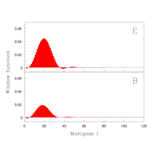
FIG. 1.: The window function corresponding to the B2001 measurement of ${\delta T^{2}}_{\l}^{E}$ for $\l=20$. Upper panel shows sensitivity to $E$-power (wanted) and lower panel shows sensitivity to $B$-power (unwanted — what we call “leakage”).

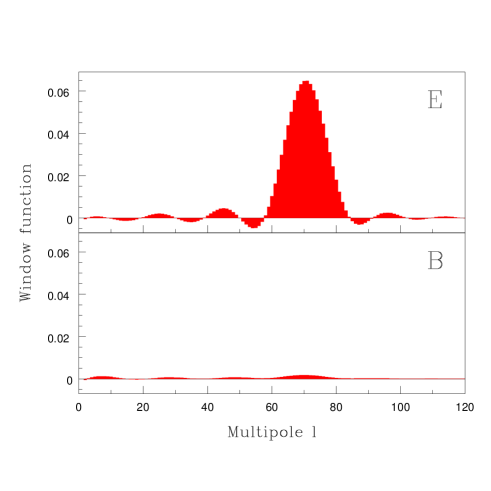
FIG. 2.: Same as Figure 1, but for the B2001 $E$-measurement aimed at $\l=70$.

A Case studies

Our five case studies are listed in Table 1. The first three cover the northern Galactic cap $b>20^{\circ}$ with successively higher sensitivity. The fourth covers a much smaller cap $b>80^{\circ}$, and the fifth covers merely a one-dimensional region: the circle defined by $b=80^{\circ}$. These case studies are not intended to be accurate forecasts for the actual performance of the experiments listed, but rather to span an interesting range in sensitivity, sky coverage and map shape. There are therefore numerous departures from realism. For instance, the actual maps from COBE, MAP and Planck will of course include the southern Galactic caps as well — apart from reducing the error bars, adding this reflection symmetry to the sky maps eliminates all leakage between even and odd $\l$-values [20], preserving the overall width of the window functions that we will present but giving them a jagged behavior where every other entry vanishes. The actual map from the Boomerang 2001 (“B2001”) experiment will not be round and will have non-uniform sensitivity. We assume uncorrelated pixel noise for simplicity. Most of the experimental sensitivities we have used are likely to be slight underestimates, being based on a single frequency channel.

In all cases, we explicitly perform the various matrix computations described in Section II. The reason that this is numerically feasible within the scope of this paper is that the large angular scales of interest here allow us to use larger and fewer pixels than the experimental teams will employ in their actual data reduction.

We will first study window functions to quantify how accurately $E$ and $B$ can be separated in various cases. We will then discuss measurement of the cross power spectrum and finally investigate how accurately approximate error bars from the Fisher matrix formalism match the results from our full numerical calculation.

B $E$ and $B$ window functions

We begin by quantifying the ability of $B2001$ and $MAP$ to separate $E$ and $B$ using $Q$- and $U$-maps. We pixelize our sky patches using the equal-area icosahedron method [33] at resolution levels 35 and 7, respectively, corresponding to 361 B2001 pixels and 561 MAP pixels. Since $Q$ and $U$ are measured for each pixel, the data vectors ${\bf x}$ have twice these lengths. We use the method given by equation (15) with ${\bf B}={\bf F}^{-1/2}$ unless otherwise specified. We compute fiducial power spectra $C_{\l}^{T}$, $C_{\l}^{E}$ and $C_{\l}^{TE}$, with the CMBFAST software [35] using cosmological parameters from the “concordance” model from [36], which provides a good fit to existing CMB and large scale structure data. We set $C_{\l}^{TB}=C_{\l}^{EB}=0$. Although the true $B$-power spectrum may be close to zero, we set $C_{\l}^{B}=C_{\l}^{E}$ in our fiducial model since we wish to highlight geometrical effects. Since this prior is $E/B$-symmetric, any asymmetries between $E$ and $B$ in our resulting window functions and error bars will be due to geometry alone. We eliminate sensitivity to offsets by projecting out the mean (monopole) for the $T$, $Q$ and $U$ maps separately, as described in the Appendix of [20].

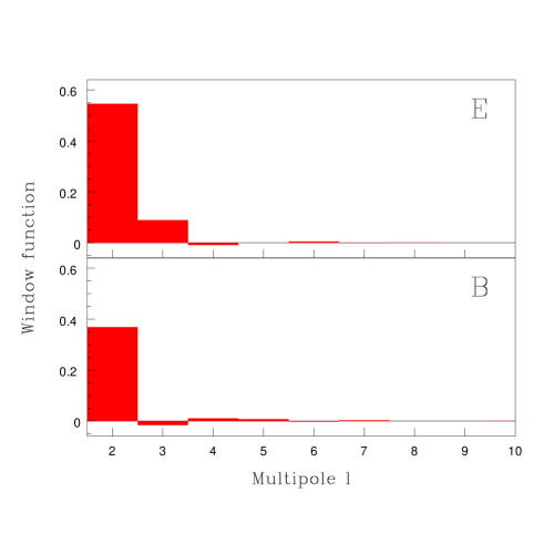
FIG. 3.: Same as Figure 1, but for the MAP $E$-measurement aimed at $\l=2$.

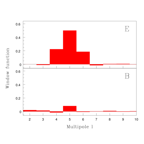
FIG. 4.: Same as Figure 1, but for the MAP $E$-measurement aimed at $\l=5$.

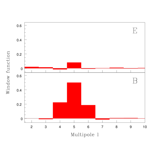
FIG. 5.: Same as Figure 1, but for the MAP measurement of ${\delta T^{2}}_{\l}^{B}$ for $\l=5$.

1 Dependence on sky coverage and angular scale

Figures 1-5 show a sequence of sample window functions for B2001 and MAP. Note that it is possible for window functions to go slightly negative for the decorrelation method ${\bf B}={\bf F}^{-1/2}$ used here, whereas the method given by ${\bf B}={\bf I}$ guarantees non-negative windows. Just as for the unpolarized case, the window function width $\Delta\l$ is seen to be fairly independent of the target multipole $\l$, essentially scaling as the inverse size of the sky patch covered [37].

The amount of leakage of $B$-power into our $E$ estimate is quantified by the lower panels in Figures 1-4, and is seen to decrease as smaller scales are probed. Figure 5 targets $B$-polarization and looks like Figure 4 with the two panels swapped, thereby showing that the leakage problems between $E$ and $B$ are quite symmetric. The smaller the area under the unwanted half of the window function, the better our method separates $E$ and $B$. As a simple quantitative measure of this power leakage, let us therefore define a $2\times 2$ leakage matrix $\L^{\l}$ for each $\l$, given by

$$\L^{\l}_{PP^{\prime}}\equiv\sum_{\l^{\prime}=2}^{\ell_{\rm max}}W^{\l P}_{\l^{\prime}P^{\prime}},$$ (18)

where $P$ and $P^{\prime}$ take the values $E,B$. In other words, the four components of this leakage matrix are the areas under the four histograms in Figure 4 and 5. If $\L^{\l}_{EE}=\L^{\l}_{BB}=1$ and $\L^{\l}_{EB}=\L^{\l}_{BE}=0$, i.e., if $\L^{\l}={\bf I}$, then there is on average no leakage at all between $E$ and $B$. For the simple case of complete sky coverage and uniform noise, all window functions become Kronecker delta functions, $W^{\l P}_{\l^{\prime}P^{\prime}}=\delta_{PP^{\prime}}\delta_{\l\l^{\prime}}$, and we verified that this happens numerically as a test of our software (in practice, it works only when $\l,\l^{\prime}$ are smaller than the scale corresponding to the pixel separation, i.e., when the map is adequately oversampled). This simple case thus gives the ideal case $\L^{\l}={\bf I}$, but we will return in Section III C to a method producing this desirable result even for partial sky coverage.

FIG. 6.: The amount of leakage of $B$-power into the $E$-power spectrum estimates is shown for the cases of B2001 (top panel, solid), CIRCLE (top panel, dashed) and MAP (bottom panel, solid). These curves show the $B/E$ ratio ($\L^{\l}_{EB}/\L^{\l}_{EE}$) for the $E$-estimates. The corresponding curves for leakage in the reverse direction (the $E/B$-ratio $\L^{\l}_{BE}/\L^{\l}_{BB}$ for the $B$-estimates) are visually identical.

To assess how the leakage depends on sky coverage and angular scale, we plot the leakage for B2001, MAP and CIRCLE as a function of $\l$ in Figure 6. Specifically, we plot the ratios of unwanted to wanted contributions, i.e., $\L^{\l}_{EB}/\L^{\l}_{EE}$ and $\L^{\l}_{BE}/\L^{\l}_{BB}$. These plots show three noteworthy results:

1. The situation for $E$ and $B$ is rather symmetric, with essentially equal leakage from $B$ to $E$ as vice versa.

2. The leakage drops with $\l$.

3. The B2001 and MAP curves have roughly similar shape apart from a scaling of the horizontal axis by a factor $\sim 7$, corresponding to the map size ratio.

Result 2 is expected since map boundary effects (incomplete sky coverage) are the reason that we cannot separate $E$ and $B$ perfectly — these boundary effects become less important as angular scales much smaller than the map are considered. In the small-scale limit where sky curvature and discreteness of $\l$ become irrelevant, one would expect result 3 as well, since there is no other $\l$-scale in the problem than the window function width $\Delta\l$, of order the inverse size of the map. If $\theta$ denotes the diameter of our circular sky patches in radians, then the FWHM window widths for B2001 and MAP are roughly fit by $\Delta\l\approx 5/\theta$, and the figures show that the leakage ratio drops below $15\%$ for $\l\mathrel{\hbox to0.0pt{\lower 3.0pt\hbox{$\mathchar 536\relax$}\hss}\raise 2.0pt\hbox{$\mathchar 318\relax$}}2\Delta\l$. (Things are different for the CIRCLE case, which we defer to Section III B 2.)

In conclusion, we have found that $E/B$ separation works well for $\l\gg\Delta\l$.

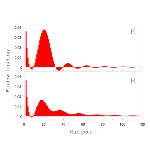
FIG. 7.: Same as Figure 1, but for the CIRCLE $E$-measurement aimed at $\l=20$.

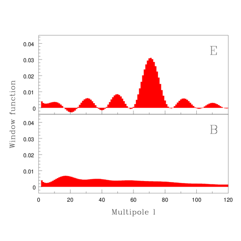
FIG. 8.: Same as Figure 1, but for the CIRCLE $E$-measurement aimed at $\l=70$.

2 Dependence on map shape

Above we studied how leakage problems depend on map size. To assess how they depend on map shape, we will now compare two rather extreme examples: a disc and a circle. The B2001 and CIRCLE maps have the same diameter and thus probe comparable angular scales. However, whereas the B2001 map is truly two-dimensional, the CIRCLE map is essentially one-dimensional, containing merely a single strip of pixels along the circumference. The two current polarization experiments POLAR [10] and PIQUE [7] both use ring-shaped maps, and this important case has also been extensively studied theoretically [11].

We pixelize our CIRCLE map with 360 equispaced pixels around the circle. Sample CIRCLE window functions are shown in Figures 7 and 8. It is seen that the CIRCLE windows are generally broader (with larger $\Delta\l$) than their B2001 counterpart, which agrees with the well-known rule of thumb [23] that the narrowest dimension of a map is the limiting factor. We also see that whereas the B2001 leakage reduced on smaller scales, things do not get correspondingly better for the CIRCLE case. This explains the dashed curve in Figure 6, which shows that substantial leakage persists even on small scales. In Section III C, we will describe how leakage can be further reduced.

In conclusion, we find that although ring maps do allow an interesting degree of $E/B$-separation, a two-dimensional map works better in this regard.

3 Dependence on sensitivity

Above we investigated how $E/B$-leakage was affected by map size and shape. To assess the effect of map sensitivity, we compare our COBE, MAP and Planck examples. These have identical sky coverage and pixelization, so the only difference is the sensitivity per unit area which increases dramatically from COBE to MAP to Planck. We refrain from plotting the three leakage curves, since they look visually identical to the MAP curve in Figure 6. This means that the effect of sensitivity on $E/B$ separation is negligible compared to the effect of sky coverage. In other words, it depends mainly on geometry and only weakly on the (sensitivity-dependent) details of the pixel weighting.

Generally, the quadratic estimator method strives to minimize error bars by reducing leakage from multipoles and polarization types with substantial power. In a situation where sample variance is dominant, this tends to make windows slightly lopsided, with a wider wing towards the direction where power decreases — in most cases towards the right. Conversely, in a situation where detector noise is dominant, windows tend to be slightly lopsided in the opposite sense, since noise power normally increases on smaller scales.

C Disentangling $E$ and $B$ better

Above we have seen that the $E$ and $B$ power spectra can be fairly accurately separated on angular scales $\l\gg\Delta\l$ with the decorrelated quadratic estimator method. Here we will argue that it is in some cases possible to do even better. Our motivation for pursuing this is that whereas broad windows in the $\l$-direction are easy to interpret (corresponding simply to a smoothing of the power spectrum), the mixing of different polarization types is rather annoying and complicates the interpretation of results.

Each choice of ${\bf B}$ in equation (15) corresponds to a different way of plotting the results. Which is the best choice?

If the goal is to use the measured band power estimates in ${\bf p}$ to constrain cosmological parameters, the choice is irrelevant. Any two methods using invertible ${\bf B}$-matrices of course retain exactly the same cosmological information, since it is possible to go back and forth between the corresponding two ${\bf p}$-vectors by multiplying by ${\bf B}_{2}{\bf B}_{1}^{-1}$ or ${\bf B}_{1}{\bf B}_{2}^{-1}$. This means that the likelihood function for cosmological parameters will be identical for the two methods.

The choice of ${\bf B}$ is therefore mainly a matter of presenting the power spectrum measurements in a clear and intuitive way. Ideally, a method would have the following properties

1. No leakage between $E$ and $B$

2. Narrow window functions

3. Uncorrelated error bars

Unfortunately, these three properties are only achievable simultaneously (without information loss) for the case of complete sky coverage. As discussed in [32], the choice ${\bf B}={\bf F}^{-1/2}$ in equation (15) achieves 3 and does a fairly good job on 2, giving window functions with the fundamental $\l$-resolution corresponding to the sky coverage. Above we saw that this gives a leakage between $E$ and $B$ that is substantial on scales corresponding to the size of the survey and approaches zero on substantially smaller scales.

In contrast, the choice ${\bf B}={\bf F}^{-1}$ in equation (15) achieves 1 and 2 perfectly, but at the cost of producing measurements that are difficult to interpret because the error bars are typically anticorrelated and huge [32]. However, these problems are to a large extent caused by eliminating the rather benign leakage between different $\l$-values. We will now describe a less aggressive method that merely targets the $E/B$-leakage. Specifically, let us insist that the leakage matrices $\L^{\l}={\bf I}$ for all $\l$.

Let us define the disentangling method as the one given by equation (15) with the ${\bf B}$-matrix chosen as

$${\bf B}_{ii^{\prime}}={\bf B}_{{\bf P}\l{\bf P}^{\prime}\l^{\prime}}\equiv\sum_{P^{\prime\prime}}(\L_{\l}^{-1})_{PP^{\prime\prime}}{\bf F}^{-1/2}_{{\bf P}^{\prime\prime}\l{\bf P}^{\prime}\l^{\prime}}.$$ (19)

Here we have once again combined $P$ and $\l$ into a single index $i=({\ell_{\rm max}}-1)(P-1)+\l-1$. It is easy to show that this method gives ideal leakage matrices $\L^{\l}={\bf I}$ if the leakage matrices in equation (19) were computed using ${\bf B}={\bf F}^{-1/2}$. This means that the unwanted half of the window function averages to zero. A similar scheme was found to work well for disentangling three types of power in a galaxy redshift survey [38].

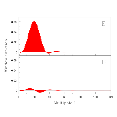
FIG. 9.: Same as Figure 1, but after applying our disentanglement method.

FIG. 10.: Curves showing leakage of $B$-power into estimates of $E$ are plotted for B2001 before (solid) and after (dashed) applying out disentanglement method. In this plot, leakage has been computed by taking absolute values of the window functions — otherwise the dashed curve would be identically zero. For example, the value of the dashed curve at $\l=20$ can be interpreted simply as the ratio of shaded area in the two panels of Figure 9.

We test this method for our B2001 example, and a sample disentangled window function is shown in Figure 9. Comparing this with Figure 1, which targeted the same multiple, we see that the leakage (lower panel) has been substantially reduced and oscillates around zero. On very large angular scales $\l\sim\Delta\l$, this undesirable half of the window function remains substantial even though it by construction averages to zero. On small scales, however, the unwanted part of the window function is found to be consistently near zero, not merely on average. This is because both the desirable and the undesirable halves of the initial window function before disentanglement have essentially the same shape, so that our disentanglement process will cancel them out almost completely. To quantify how well the this process works, Figure 10 shows leakage curves with the leakage matrix redefined with absolute values:

$${\bf\tilde{L}}^{\l}_{PP^{\prime}}\equiv\sum_{\l^{\prime}=2}^{\ell_{\rm max}}\left|W^{\l P}_{\l^{\prime}P^{\prime}}\right|,$$ (20)

(Without taking absolute values, the disentanglement method would by construction be diagnosed with zero leakage.)

Although this method is likely to be adequate for practical applications, it is possible to disentangle $E$ and $B$ still better if necessary, at the price of larger error bars. The Fisher matrix ${\bf F}$ generally becomes singular if the bands used are much narrower than $\Delta\l$. If the sky coverage is large enough that $\Delta\l$ is narrower than features of interest in the power spectra, is it convenient to choose bands of width around $\Delta\l$ instead of width one (solving for each multipole separately). Since this produces an invertible Fisher matrix, perfect disentanglement is achievable by setting ${\bf B}={\bf F}^{-1}$ in equation (15), giving only a modest increase in error bars and rather slight anticorrelations between neighboring bands. The resulting measurements can then be made uncorrelated separately for $E$ and $B$, by multiplying by the inverse square roots of the corresponding two covariance matrices, thereby broadening the $\l$-windows back to their natural widths.

D Measuring the cross power spectrum

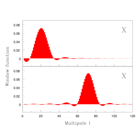
FIG. 11.: Window functions for measuring the cross power spectrum are shown for the B2001 case, targeting $\l=20$ (top) and $\l=70$ (bottom).

The three cross power spectra $C_{\l}^{TE}$, $C_{\l}^{TB}$ and $C_{\l}^{EB}$, which we will denote $C_{\l}^{X}$, $C_{\l}^{Y}$ and $C_{\l}^{Z}$ for brevity, can be measured using the basic decorrelated quadratic estimators given by equation (15) without any modification. However, as we will now discuss, this is not necessarily the most desirable approach.

To measure the cross power spectrum $C_{\l}^{X}$, our data vector ${\bf x}$ must contain both unpolarized and polarized measurements as in equation (1). These may be either from a single experiment or from separate unpolarized and polarized ones. As reviewed in Appendix A, this gives a covariance matrix of the form

$${\bf C}\equiv\langle{\bf x}{\bf x}^{t}\rangle=\left(\begin{tabular}[]{ccc}$\langle{\bf T}{\bf T}^{t}\rangle$&$\langle{\bf T}{\bf Q}^{t}\rangle$&$\langle{\bf T}{\bf U}^{t}\rangle$\\[2.0pt] $\langle{\bf Q}{\bf T}^{t}\rangle$&$\langle{\bf Q}{\bf Q}^{t}\rangle$&$\langle{\bf Q}{\bf U}^{t}\rangle$\\[2.0pt] $\langle{\bf U}{\bf T}^{t}\rangle$&$\langle{\bf U}{\bf Q}^{t}\rangle$&$\langle{\bf U}{\bf U}^{t}\rangle$\\[2.0pt] \end{tabular}\right)$$ (21)

which generically has non-vanishing elements in all the off-diagonal blocks. When we try to measure one of the parameters $p_{i}$ corresponding to the cross power spectrum $C_{\l}^{X}$, the matrix ${\bf P}_{i}=\partial{\bf C}/\partial p_{i}$ will vanish except in the $T-Q$ and $T-U$ cross-correlation blocks, since these are the only ones that depend on $C_{\l}^{X}$. However, since ${\bf C}$ is a full matrix, the quadratic estimator ${\bf Q}_{i}\propto{\bf C}^{-1}{\bf P}_{i}{\bf C}^{-1}$ (as well as decorrelated or disentangled variants thereof) will also be a full matrix, without any vanishing blocks. This means that the estimates $q_{i}$ of the cross power spectrum will involve not only data combinations like $T_{j}Q_{k}$ and $T_{j}U_{k}$, but also terms like $T_{j}T_{k}$ and $Q_{j}Q_{k}$. In other words, the measured cross-correlation involves, among other things, the correlation of the temperature map with itself! The same peculiarity applies to the maximum-likelihood method, which is simply an iterated version of the quadratic method.

We will now give a simple example illustrating why this happens, as well as argue that it is avoidable and sometimes undesirable.

1 A complicated way to measure correlation

As an illustrative toy model, let us temporarily assume that our data vector ${\bf x}$ consists of merely two numbers, the measurements of $T$ and $E$ for a given multipole $(\l,m)$ extracted from an all-sky map. Consider the simple case where $C_{\l}^{T}=C_{\l}^{E}=1$ — the general case will follow from our result by a trivial scaling. This means that the data covariance matrix takes the form

$${\bf C}\equiv\langle{\bf x}{\bf x}^{t}\rangle=\left(\begin{tabular}[]{cc}$\langle C_{\l}^{T}\rangle$&$\langle C_{\l}^{X}\rangle$\\[2.0pt] $\langle C_{\l}^{X}\rangle$&$\langle C_{\l}^{E}\rangle$\end{tabular}\right)=\left(\begin{tabular}[]{cc}$1$&$r$\\[2.0pt] $r$&$1$\\[2.0pt] \end{tabular}\right),$$ (22)

where $r\equiv C_{\l}^{X}/[C_{\l}^{T}C_{\l}^{E}]^{1/2}$ is the dimensionless correlation coefficient between $T$ and $E$. We have only three parameters to measure in our toy example, ${\bf p}=(C_{\l}^{T},C_{\l}^{E},C_{\l}^{X})$, so the matrices ${\bf P}_{i}=\partial{\bf C}/\partial p_{i}$ are

$${\bf P}_{1}=\left(\begin{tabular}[]{cc}$1$&$0$\\[2.0pt] $0$&$0$\\[2.0pt] \end{tabular}\right),\quad{\bf P}_{2}=\left(\begin{tabular}[]{cc}$0$&$0$\\[2.0pt] $0$&$1$\\[2.0pt] \end{tabular}\right),\quad{\bf P}_{3}=\left(\begin{tabular}[]{cc}$0$&$1$\\[2.0pt] $1$&$0$\\[2.0pt] \end{tabular}\right).$$ (23)

Substituting this and equation (22) into equation (17) gives the Fisher matrix

r2212−r−r−r1+r2),𝐅1superscript1superscript𝑟22fragments superscript𝑟2212fragmentsrfragmentsrfragmentsrfragments1r2{\bf F}={1\over(1-r^{2})^{2}}\left(\begin{tabular}[]{ccc}${1\over 2}$&${r^{2}\over 2}$&$-r$\\[2.0pt] ${r^{2}\over 2}$&${1\over 2}$&$-r$\\[2.0pt] $-r$&$-r$&$1+r^{2}$\\[2.0pt] \end{tabular}\right),

12r22-r12r22-r (24)

with inverse

r21rrr1+r22).superscript𝐅112fragments fragmentsr21𝑟𝑟𝑟1superscript𝑟22{\bf F}^{-1}={1\over 2}\left(\begin{tabular}[]{ccc}$1$&$r^{2}$&$r$\\[2.0pt] $r^{2}$&$1$&$r$\\[2.0pt] $r$&$r$&${1+r^{2}\over 2}$\\[2.0pt] \end{tabular}\right).

1r2r1r2r (25)

Substituting the above equations into equation (15) and using the method given by ${\bf B}={\bf F}^{-1}$, the resulting unbiased estimators take the simple form

$${\bf Q}_{1}=\left(\begin{tabular}[]{cc}$1$&$0$\\[2.0pt] $0$&$0$\\[2.0pt] \end{tabular}\right),\quad{\bf Q}_{2}=\left(\begin{tabular}[]{cc}$0$&$0$\\[2.0pt] $0$&$1$\\[2.0pt] \end{tabular}\right),\quad{\bf Q}_{3}={1\over 2}\left(\begin{tabular}[]{cc}$0$&$1$\\[2.0pt] $1$&$0$\\[2.0pt] \end{tabular}\right).$$ (26)

This is not surprising, since no other estimators could possibly be unbiased ($\langle{\bf q}\rangle={\bf p}$) when only one spherical harmonic mode is used. As soon as more modes are available, however, things can (and generally do) get more complicated. Consider, the case where ${\bf x}$ consists of four rather than two measurements for our multipole, — temperature measurements $T_{1}$ and $T_{2}$ and $E$-polarization measurements $E_{1}$ and $E_{2}$. The obvious guess would be that and estimator of $C_{\l}^{X}$ should involve only cross terms ($T_{1}E_{1}$, $T_{1}E_{2}$ and $T_{2}E_{2}$). However, terms such as $T_{1}^{2}-T_{2}^{2}$ and $E_{1}^{2}-E_{2}^{2}$ will have a vanishing average, and can therefore be added to any estimator without biasing it. As we saw above, precisely this generically happens in our minimum-variance estimator, since it helps reduce the estimator variance if our four measurements have different noise variances.

This can also be understood as follows. Repeating the derivation of equation (26) when there are $n$ measurement of $T$ and $E$ for our mode, perhaps with different variances, shows that the zeroes in equation (26) will be replaced by $n\times n$ blocks that generally not vanish — merely their traces will.

2 A simpler way

Apart from being surprisingly complicated to compute and interpret, the basic quadratic estimators of equation (10) also have drawback related to systematic errors. If the estimated cross-power spectrum involves components of the unpolarized and polarized power spectra that are supposed to cancel out to reduce the variance, there is a risk that systematic errors from these two autocorrelations propagate into and contaminate the cross-correlation measurements. For this reason, an interesting alternative is to use an estimator for the cross-power spectrum that does not have this funny property, i.e., that contains only cross-terms. A simple way to construct such an estimator is to use equation (15) with the fiducial power spectrum $C_{\l}^{X}$ set equal to zero. This will make ${\bf C}$ and ${\bf C}^{-1}$ block diagonal, so the ${\bf Q}$-matrices of equation (15) acquire the same block structure as the ${\bf P}$-matrices. The estimators of $C_{\l}^{X}$ therefore involve only cross terms.

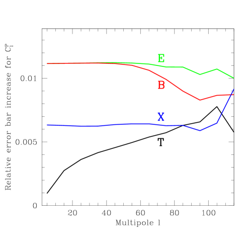
FIG. 12.: The low cost of simplicity. The curves show the relative increase of the error bars on the four power spectra when the fiducial model is replaced by one with ${\bf C}_{\l}^{X}=0$, thereby eliminating potential systematic errors as described in the text.

It is noteworthy that this issue applies not only to estimation of $C_{\l}^{X}$, but to measuring $C_{\l}^{T}$, $C_{\l}^{E}$ and $C_{\l}^{B}$ as well. If the fiducial power spectrum has $C_{\l}^{X}\neq 0$, then estimators of all four power spectra will involve using combinations of all three maps $({\bf T},{\bf Q},{\bf U})$, so setting $C_{\l}^{X}\neq 0$ when using equation (15) is an interesting simplifying option for all power spectrum estimation. We implicitly did so in Section III B by ignoring the $T$-map.

3 Which method is better?

The price we must pay for this simplification is a slight increase in error bars. This is quantified in Figure 12 for the B2001 case. We computed the error bars on the four standard power power spectra for the unbiased method with both weighting schemes (assuming the true $C_{\l}^{X}$ for our concordance model and assuming $C_{\l}^{X}=0$). The figure shows the ratios (minus one), and illustrates that the simplification typically comes at a very low cost — an error bar increase of order a percent. In light of this and the potential peril of systematic errors, the simpler method appears preferable in practice. Returning to the most general case of estimating six joint power spectra, it is thus prudent to set all three cross power spectra to zero in the fiducial model: $C_{\l}^{X}=C_{\l}^{Y}=C_{\l}^{Z}=0$.

E Error bars

Up until now, we have focused on the issue of window functions. Let us now turn to the complementary issue of error bars. A large number of papers, for instance [2, 5, 6, 16, 39, 40, 41, 42, 43], have made forecasts for how accurately upcoming polarization experiments can constrain cosmological parameters. These estimates all assumed that the accuracy of the recovered polarized power spectra $(C_{\l}^{T},C_{\l}^{E},C_{\l}^{B},C_{\l}^{X})$ would be given by the $4\times 4$ covariance matrix [4]

$${\bf M}_{\l}\approx{2f_{\rm sky}^{-1}\over 2\l+1}\left(\begin{tabular}[]{cccc}$T_{\l}^{2}$&$X_{\l}^{2}$&0&$T_{\l}X_{\l}$\\[2.0pt] $X_{\l}^{2}$&$E_{\l}^{2}$&0&$E_{\l}X_{\l}$\\[2.0pt] $0$&$0$&$B_{\l}^{2}$&$0$\\[2.0pt] $T_{\l}X_{\l}$&$E_{\l}X_{\l}$&0&${1\over 2}[T_{\l}E_{\l}+X_{\l}^{2}]$\end{tabular}\right).$$ (27)

where $f_{\rm sky}$ is the fraction of the sky observed and

$$P_{\l}\equiv C_{\l}^{P}+(w^{P})^{-1}e^{\theta^{2}\l(\l+1)},\quad P=T,E,B,X,$$ (28)

if the experimental beam is Gaussian with width $\theta$ in radians (the full-width-half-maximum is given by FWHM$=\sqrt{8\ln 2}\>\theta$). Here the sensitivity measure $1/w^{P}$ is defined as [44] the noise variance per pixel times the pixel area in steradians for $P=T,E,B$. For the case of the $EB$ cross power spectrum, $w^{X}=(w^{T}w^{E})^{1/2}$. Equation (28) can be interpreted as simply giving the total power from CMB (first term) and detector noise (second term). For our examples, we take $w^{T}=w^{E}=w^{B}=1/($FWHM$\>\sigma)^{2}$, where FWHM and $\sigma$ are the resolution and noise values listed in Table 1.

The approximation of equation (27) has been shown to be exact for the special case of complete sky coverage $(f_{\rm sky}=1)$ [2], and the same result follows from the Fisher information matrix formalism [6]. The factor $(2\l+1)f_{\rm sky}$ can be interpreted as the effective number of uncorrelated modes per multipole, and the other factor as giving the covariance per mode.

The approximation that the number of uncorrelated modes scales as $f_{\rm sky}$ is both natural and well-motivated [45]. How accurate is it in practice? Our calculations enable us to address this issue quantitatively. Figure 13 shows the ratio of the approximate error bars from equation (27) to the exact error bars from equation (14) for the four power spectra (the ratios of the square roots of the corresponding elements on the covariance matrix diagonals). To ensure a fair comparison, we used the uncorrelated method given by equation (15) with ${\bf B}={\bf F}^{-1/2}$ — the ${\bf B}={\bf F}^{-1}$ and maximum-likelihood methods give larger anticorrelated error bars, whereas the ${\bf B}={\bf I}$ method gives smaller correlated ones. It is seen that the approximation of equation (27) is generally quite accurate when $\l\gg\Delta\l$ and $\l\ll{\ell_{\rm max}}-\Delta\l$, i.e., for multipoles well away from the two endpoints of the range computed. This means that forecasts made using the approximation of equation (27) should be viewed as quite accurate except on scales comparable to the survey size.

For the case where all six power spectra are measured jointly, equation (27) is generalized so that the matrix in parenthesis gets replaced by the following one (suppressing the subscript $\l$ for brevity):

$$\left(\begin{tabular}[]{cccccc}$T^{2}$&$X^{2}$&$Y^{2}$&$TX$&$TY$&$XY$\\[2.0pt] $X^{2}$&$E^{2}$&$Z^{2}$&$EX$&$XZ$&$EZ$\\[2.0pt] $Y^{2}$&$Z^{2}$&$B^{2}$&$YZ$&$BY$&$BZ$\\[2.0pt] $TX$&$EX$&$YZ$&${TE+X^{2}\over 2}$&${TZ+XY\over 2}$&${EY+XZ\over 2}$\\[2.0pt] $TY$&$XZ$&$BY$&${TZ+XY\over 2}$&${TB+Y^{2}\over 2}$&${BX+YZ\over 2}$\\[2.0pt] $XY$&$EZ$&$BZ$&$\>{EY+XZ\over 2}$&$\>{BX+YZ\over 2}$&$\>{EB+Z^{2}\over 2}$\end{tabular}\right)$$ (29)

This can either be derived directly from a quadratic estimator as in [4] or by computing the inverse Fisher information matrix as in [6].

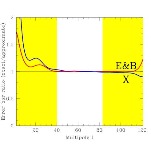
FIG. 13.: The curves show the ratio of the actual error bars to those computed with the approximation of equation (27). The approximation is seen to be excellent for multipoles more than a couple of bandwidths $\Delta\l$ away from the two endpoints of the $\l$-range computed (outside shaded regions).

IV Discussion

We have presented a method for measuring CMB polarization power spectra given incomplete sky coverage and tested it with a number of simulated examples.

A What have we learned?

The issue of measuring the T power spectrum has been extensively treated in prior literature. An added challenge when measuring the E and B power spectra is leakage between the two caused by incomplete sky coverage. We quantified this leakage for the first time, and found that it is rather insensitive to experimental noise levels and depends mainly on geometry. Specifically, we found the leakage to depend mainly on the ratio $\l/\Delta\l$, where $\Delta\l$ is the characteristic window function width and scales roughly as the inverse size of the sky patch in its narrowest direction. We introduced a disentanglement method which reduced the leakage to $5\%-10\%$ for $\l\mathrel{\hbox to0.0pt{\lower 3.0pt\hbox{$\mathchar 536\relax$}\hss}\raise 2.0pt\hbox{$\mathchar 318\relax$}}\Delta\l$, and described how it could be pushed to zero if necessary, at the cost of larger error bars.

We found that when measuring the X power spectrum, the basic quadratic estimator produces a surprisingly complicated answer, involving not only temperature-polarization cross terms, but also, e.g., autocorrelations of the temperature map with itself. This is unfortunate, since it can make the measured power spectrum more sensitive to systematic errors. Especially if the temperature and polarization maps are made by two different experiments, systematics should be uncorrelated between the two and therefore not contribute to the cross term average. The maximum-likelihood method exhibits the same problem. This can affect $E$- and $B$-polarization estimation as well, by giving non-zero weight to the unpolarized map. The problem is eliminated by simply using vanishing cross-power in the fiducial model. We find that this is desirable in practice, since the resulting information loss causes error bars to increase only by negligle amounts, at the percent level.

Finally, we found that on scales substantially smaller than the sky patch, the error bars for the $F^{-1/2}$-method were accurately fit by the approximation of equation (27), where variance scales inversely with sky coverage.

B Relation to other methods

The quadratic estimator (QE) method is closely related to the maximum-likelihood (ML) method: the latter is simply the quadratic estimator method with ${\bf B}={\bf F}^{-1}$ in equation (15), iterated so that the fiducial (“prior”) power spectrum equals the measured one [21]. The ML method has the advantage of not requiring any prior to be assumed. The QE method has the advantage of being faster (no iteration) and simpler to interpret — since it is quadratic rather than highly non-linear, the statistical properties the measured band power vector ${\bf q}$ can be computed analytically. This allows the likelihood function to be computed directly from ${\bf q}$ (as opposed to ${\bf x}$), in terms of generalized $\chi^{2}$-distributions [46].

Both methods are unbiased, but they may differ as regards error bars. The QE method can produce inaccurate error bars if the prior is inconsistent with the actual measurement. The ML method Fisher matrix can produce inaccurate error bar estimates if the measured power spectra have substantial scatter due to noise or sample variance, in which case they are unlikely to describe the smoother true spectra. A good compromise is therefore to iterate the QE method once and choose the second prior to be a rather smooth model consistent with the original measurement. In addition, as mentioned above, we found that it is useful to set the $X$ power spectrum to zero in the prior.

The difference between the QE and ML methods is often small in practice, which can be understood as follows. Since the QE method can be shown to be lossless if the prior equals the truth, thereby minimizing the error bars, small departures from the true prior merely destroy information to second order. This is also why adopting a prior without $X$ power inflated the error bars so little.

The analysis of weak gravitational lensing data is rather analogous to that of CMB polarization, since the projected shear field can be decomposed into components corresponding to $E$ and $B$. Recent lensing work cast in this language has included both theoretical predictions for various effects [47, 48] and data analysis issues [49, 50]. In particular, no $E/B$ leakage was detected at the 10% level when the ML method was applied to simulated examples [49], which can be understood from our present results since the band power bins used were substantially broader than $\Delta\l$[49] and mainly on scales $\l\gg\Delta\l$.

C Outlook

Our basic results are good news: although polarized power spectrum estimation adds several complications to the non-polarized case, they can all be dealt with using the techniques we have described. However, much theoretical work remains to be done. Here are a couple of examples of areas deserving further study:

• The effects of pixel shape and size in the mapmaking process needs to be quantified, and is likely to be more important for the polarized case.

• Although the methods we have discussed apply equally well to measuring the power spectra of non-Gaussian signals (the only change is that the error bars will no longer be given by equation (14)), non-Gaussian signals contain more information than is contained in their power spectra. Polarized non-Gaussian fluctuations are expected from microwave foregrounds [52, 53, 54], secondary anisotropies [55], topological defects [47] and CMB lensing [48], and only a small number of papers have so far addressed the issue of how to best measure such non-Gaussian signatures in practice [56, 57, 58].

First and foremost, however, we need a detection of CMB polarization!

The authors wish to thank Wayne Hu, Brian Keating, Ue-Li Pen and Matias Zaldarriaga for helpful comments, and the B2001, PIQUE and POLAR teams for encouraging us to write up these calculations. Support for this work was provided by NASA grant NAG5-9194, NSF grant AST00-71213 and the University of Pennsylvania Research Foundation.

A Computing the polarization covariance matrix

This Appendix is intended for the reader who wishes to write software to explicitly compute the polarization covariance matrix. The complete formalism for describing CMB polarization was presented in [1, 2], and extended with a number of useful explicit formulas in [11]. However, a number of practical details are not covered in the literature, e.g., the rotation angles and degenerate cases, so we describe all steps explicitly for completeness.

Let the 3-dimensional vector ${\bf x}_{i}$ denote the three measurable quantities for the $i^{th}$ pixel:

$${\bf x}_{i}\equiv\left(\begin{tabular}[]{c}$T_{i}$\\ $Q_{i}$\\ $U_{i}$\end{tabular}\right).$$ (A1)

The $3\times 3$ covariance matrix between two such vectors at different points can be written

$$\langle{\bf x}_{i}{\bf x}_{j}^{t}\rangle={\bf R}(\alpha_{ij}){\bf M}(\widehat{\bf r}_{i}\cdot\widehat{\bf r}_{j}){\bf R}(\alpha_{ji})^{t},$$ (A2)

Here ${\bf M}$ is the covariance using a $(Q,U)$-convention where the reference direction is the great circle connecting the two points, and the rotation matrices given by

0cos2αsin2α0−sin2αcos2α)𝐑𝛼fragments 0fragments2αfragments2α0fragments2αfragments2α{\bf R}(\alpha)\equiv\left(\begin{tabular}[]{ccc}$1$&$0$&$0$\\[2.0pt] $0$&$\cos 2\alpha$&$\sin 2\alpha$\\[2.0pt] $0$&$-\sin 2\alpha$&$\cos 2\alpha$\\[2.0pt] \end{tabular}\right)

100100 (A3)

accomplish a rotation into a global reference frame where the reference directions are meridians. The full $(3n)\times(3n)$ map covariance matrix is readily assembled out of the $3\times 3$ blocks of equation (A2) by looping over all pixel pairs. A powerful probe for bugs is making sure that this large matrix is positive definite.

1 Computing the rotation angles

As we will see, computing the magnitudes of the rotation angles $\alpha_{ij}$ is straightforward, whereas getting the correct sign is somewhat subtle.

The great circle connecting the two pixels has the unit normal vector

$$\widehat{\bf r}_{ij}\equiv{\widehat{\bf r}_{i}\times\widehat{\bf r}_{j}\over|\widehat{\bf r}_{i}\times\widehat{\bf r}_{j}|}.$$ (A4)

Similarly, the meridian passing though pixel $i$ (its reference circle for our global $(Q,U)$-convention) has the unit normal vector

$$\widehat{\bf r}_{i}^{*}\equiv{\widehat{{\bf z}}\times\widehat{\bf r}_{i}\over|\widehat{{\bf z}}\times\widehat{\bf r}_{i}|},$$ (A5)

where $\widehat{{\bf z}}=(0,0,1)$ is the unit vector in the $z$-direction. The magnitude of $\alpha_{ij}$, the rotation angle for pixel $i$, is simply the angle between these two great circles, so $\cos\alpha_{ij}=\widehat{\bf r}_{ij}\cdot\widehat{\bf r}_{i}^{*}$. The sign of $\alpha_{ij}$ is defined so that a positive angle corresponds to clockwise rotation at the pixel (at $\widehat{\bf r}_{i}$). We therefore compute the cross product of the two circle normals, which has the property that

$$\widehat{\bf r}_{ij}\times\widehat{\bf r}_{i}^{*}=\widehat{\bf r}_{i}\sin\alpha_{ij}.$$ (A6)

(Since both $\widehat{\bf r}_{ij}$ and $\widehat{\bf r}_{i}^{*}$ are by construction perpendicular to $\widehat{\bf r}_{i}$, their cross product will be either aligned or anti-aligned with $\widehat{\bf r}_{i}$.) Dotting equation (A6) with $\widehat{\bf r}_{i}$ and performing some vector algebra gives

$$\sin\alpha_{ij} = (\widehat{\bf r}_{ij}\times\widehat{\bf r}_{i}^{*})\cdot\widehat{\bf r}_{i}\propto[(\widehat{\bf r}_{i}\times\widehat{\bf r}_{j})\times(\widehat{\bf r}_{i}\times\widehat{{\bf z}})]\cdot\widehat{\bf r}_{i}$$ (A7)

$$= [(\widehat{\bf r}_{i}\times\widehat{\bf r}_{j})\cdot\widehat{{\bf z}}]\>\widehat{\bf r}_{i}\cdot\widehat{\bf r}_{i}\propto\widehat{\bf r}_{ij}\cdot\widehat{{\bf z}},$$ (A8)

where the omitted proportionality constants are positive. $\alpha_{ij}$ therefore has the same sign as the $z$-coordinate of $\widehat{\bf r}_{ij}$, and is given by

$$\alpha_{ij}=\cases{+\cos^{-1}\left(\widehat{\bf r}_{ij}\cdot\widehat{\bf r}_{i}^{*}\right)&if $\widehat{\bf r}_{ij}\cdot\widehat{{\bf z}}>0$,\cr\vskip 4.0pt\cr-\cos^{-1}\left(\widehat{\bf r}_{ij}\cdot\widehat{\bf r}_{i}^{*}\right)&if $\widehat{\bf r}_{ij}\cdot\widehat{{\bf z}}<0$.}$$ (A9)

For generic pairs of directions, equation (A9) gives the two rotation angles $\alpha_{ij}$ and $\alpha_{ji}$ needed for equation (A2). However, it breaks down for the three special cases $\widehat{\bf r}_{i}\times\widehat{\bf r}_{j}={\bf 0}$, $\widehat{\bf r}_{i}\times\widehat{{\bf z}}={\bf 0}$ and $\widehat{\bf r}_{j}\times\widehat{{\bf z}}={\bf 0}$. If $\widehat{\bf r}_{i}\times\widehat{\bf r}_{j}={\bf 0}$, the two pixels are either identical or on diametrically opposite sides of the sky. Hence any great circle through $\widehat{\bf r}_{i}$ will go through $\widehat{\bf r}_{2}$ as well. We can choose this circle to be the meridian, so no rotation is needed, i.e., $\alpha_{ij}=\alpha_{ji}=0$ for this case. Indeed, ${\bf M}$ comes out diagonal for this case by symmetry, with $\langle Q_{i}U_{j}\rangle=0$ and $\langle Q_{i}Q_{j}\rangle=\langle U_{i}U_{j}\rangle$, so rotations have no effect.

If $\widehat{\bf r}_{i}\times\widehat{{\bf z}}={\bf 0}$, then the pixel is at the North or South pole, making our the global $(Q,U)$-convention undefined. The simplest remedy to this problem is to move the pixel away from the pole by a tiny amount much smaller than the beam width of the experiment.

The remainder of this section discusses some symmetry issues that the pragmatic reader may wish to skip. Equation (A9) guarantees a symmetric covariance matrix since swapping $i$ and $j$ is equivalent to transposing the result. Moreover, the two rotations ${\bf R}(\alpha_{ij})$ and ${\bf R}(\alpha_{ji})$ are nearly equal when the two pixels are much closer to each other than to the poles (the two rotations would be identical for a flat sky), which can be seen as follows. $\widehat{\bf r}_{ji}=-\widehat{\bf r}_{ij}$ from the antisymmetry of the cross product. Since $\widehat{\bf r}_{i}\approx\widehat{\bf r}_{j}$ implies that $\widehat{\bf r}_{i}^{*}\approx\widehat{\bf r}_{j}^{*}$, and $\cos^{-1}(-x)=\pi-\cos^{-1}(x)$, equation (A9) therefore gives $\alpha_{ji}\approx-(\pi-\alpha_{ij})=\alpha_{ij}-\pi.$ The extra rotation by $\pi$ has no effect, since the rotation matrix of equation (A3) depends on twice the angle.

There is a more subtle symmetry as well. Flipping the overall sign in equation (A9) will give the same covariance matrix if we redefine $U$ with the opposite sign convention. The sign convention of equation (A9) corresponds to the standard definition of $U$.

2 Computing the matrix ${\bf M}$

The ${\bf M}$-matrix depends only on the angular separation between the two pixels. It is given by

$${\bf M}(\widehat{\bf r}_{i}\cdot\widehat{\bf r}_{j})\equiv\left(\begin{tabular}[]{ccc}$\langle T_{i}T_{j}\rangle$&$\langle T_{i}Q_{j}\rangle$&$\langle T_{i}U_{j}\rangle$\\[2.0pt] $\langle T_{i}Q_{j}\rangle$&$\langle Q_{i}Q_{j}\rangle$&$\langle Q_{i}U_{j}\rangle$\\[2.0pt] $\langle T_{i}U_{j}\rangle$&$\langle U_{i}Q_{j}\rangle$&$\langle U_{i}U_{j}\rangle$\\[2.0pt] \end{tabular}\right),$$ (A10)

$$\langle T_{i}T_{j}\rangle \equiv \sum_{\l}\left({2\l+1\over 4\pi}\right)P_{\l}(z)C_{\l}^{T},$$ (A11)

$$\langle T_{i}Q_{j}\rangle \equiv -\sum_{\l}\left({2\l+1\over 4\pi}\right)F^{10}_{\l}(z)C_{\l}^{TE},$$ (A12)

$$\langle T_{i}U_{j}\rangle \equiv -\sum_{\l}\left({2\l+1\over 4\pi}\right)F^{10}_{\l}(z)C_{\l}^{BT},$$ (A13)

$$\langle Q_{i}Q_{j}\rangle \equiv \sum_{\l}\left({2\l+1\over 4\pi}\right)\left[F^{12}_{\l}(z)C_{\l}^{E}-F^{22}_{\l}(z)C_{\l}^{B}\right],$$ (A14)

$$\langle U_{i}U_{j}\rangle \equiv \sum_{\l}\left({2\l+1\over 4\pi}\right)\left[F^{12}_{\l}(z)C_{\l}^{B}-F^{22}_{\l}(z)C_{\l}^{E}\right],$$ (A15)

$$\langle Q_{i}U_{j}\rangle \equiv \sum_{\l}\left({2\l+1\over 4\pi}\right)\left[F^{12}_{\l}(z)+F^{22}_{\l}(z)\right]C_{\l}^{EB},$$ (A16)

where ${\bf z}=\widehat{\bf r}_{i}\cdot\widehat{\bf r}_{j}$ is the cosine of the angle between the two pixels under consideration. The equations for $\langle T_{i}Q_{j}\rangle$, $\langle Q_{i}Q_{j}\rangle$ and $\langle U_{i}U_{j}\rangle$ are from [11] (beware a minus sign typo in the first one) and those for $\langle T_{i}U_{j}\rangle$ and $\langle Q_{i}U_{j}\rangle$ are from [59]. $P_{\l}$ denotes a Legendre polynomial, and the functions $F^{10}$, $F^{12}$ and $F^{22}$ are [11]

$$F^{10}(z) = 2{{\l z\over(1-z^{2})}P_{\l-1}(z)-\left({\l\over 1-z^{2}}+{\l(\l-1)\over 2}\right)P_{\l}(z)\over[(\l-1)\l(\l+1)(\l+2)]^{1/2}}$$ (A17)

$$F^{12}(z) = 2{{(\l+2)z\over(1-z^{2})}P_{\l-1}^{2}(z)-\left({\l-4\over 1-z^{2}}+{\l(\l-1)\over 2}\right)P_{\l}^{2}(z)\over(\l-1)\l(\l+1)(\l+2)}$$ (A19)

$$F^{22}(z) = 4{(\l+2)P_{\l-1}^{2}(z)-(\l-1)zP_{\l}^{2}(z)\over(\l-1)\l(\l+1)(\l+2)(1-z^{2})}$$ (A21)

Here $P_{\l}$ and $P_{\l}^{2}$ denote Legendre polynomials $P_{\l}^{m}$ for the cases $m=0$ and $m=2$, respectively, which are conveniently computed using the recursion relations [60]

$$P_{\l}(z) = \cases{1&for $\l=0$,\cr\vskip 4.0pt\cr z&for $\l=1$,\cr\vskip 4.0pt\cr{(2\l-1)zP_{\l-1}(z)-(\l-1)P_{\l-2}(z)\over\l}&for $\l\geq 2$,}$$ (A22)

$$P_{\l}^{2}(z) = \cases{3(1-z^{2})&for $\l=2$,\cr\vskip 4.0pt\cr 5zP_{2}^{2}&for $\l=3$,\cr\vskip 4.0pt\cr{(2\l-1)zP_{\l-1}^{2}(z)-(\l+1)P_{\l-2}^{2}(z)\over\l-2}&for $\l\geq 4$.}$$ (A23)

The division by $(1-z^{2})$ unfortunately causes expressions  (A17)$-$(A21) to blow up numerically when $z=\pm 1$, i.e., for correlations at zero separation or between diametrically opposite pixels in the sky [61]. Taking the appropriate limits for these cases gives

$$F_{\l}^{10}(z) = 0\quad\quad\quad\quad\>\>\,\hbox{if $|z|=1$},$$ (A24)

$$F_{\l}^{12}(z) = \cases{{1\over 2}&if $z=1$,\cr\vskip 4.0pt\cr{1\over 2}(-1)^{\l}&if $z=-1$,}$$ (A26)

$$F_{\l}^{22}(z) = \cases{-{1\over 2}&if $z=1$,\cr\vskip 4.0pt\cr{1\over 2}(-1)^{\l}&if $z=-1$.}$$ (A28)

3 Including variable angular resolution

If the experimental beam is rotationally symmetric, its effect is straightforward to include even if the beam size and radial profile varies between pixels. This complication is particularly important for the case of cross-polarization, where it may be desirable to correlate polarization maps from one experiment with a temperature map from another experiment that happens to have different angular resolution.

Let $B_{i\l}$ denote the coefficients obtained from expanding the beam profile corresponding to the measurement $x_{i}$ in Legendre polynomials. For a Gaussian beam, these coefficients are accurately described by the well-known approximation

$$B_{i\l}\approx e^{-{1\over 2}\theta_{i}^{2}\l(\l+1)},$$ (A29)

where the rms beam width $\theta_{i}$ is related to the full-width-half-maximum by $\theta_{i}=$FWHM${}_{i}/\sqrt{8\ln 2}$. To compute the correlation $\langle x_{i}x_{j}\rangle$ in equation (A2), the six power spectra $C_{\l}^{P}$ are simply replaced by $C_{\l}^{P}B_{i\l}B_{j\l}$ in equations (A11) through (A16).

REFERENCES

- [1] M. Kamionkowski, A. Kosowsky, and A. Stebbins, Phys. Rev. D 55, 7368 (1997).
- [2] M. Zaldarriaga and U. Seljak, Phys. Rev. D 55, 1830 (1997).
- [3] W. Hu and M. White, New Astron 2, 323 (1997).
- [4] M. Zaldarriaga, D. N. Spergel, and U. Seljak, ApJ 488, 1 (1997).
- [5] D. J. Eisenstein, W. Hu, and Tegmark M, ApJ 518, 2 (1999).
- [6] M. Tegmark, D. J. Eisenstein, W. Hu, and A. de Oliveira-Costa, ApJ 530, 133 (2000).
- [7] M. M. Hedman, D. Barkats, J. O. Gundersen, S. T. Staggs, and B. Winstein, ApJL 548, L111 (2001).
- [8] S. T. Staggs, J. O. Gundersen, and S. E. Church 1999, astro-ph/9904062, in Microwave Foregrounds, ed. A. de Oliveira-Costa & M. Tegmark (ASP: San Francisco)
- [9] G. F. Smoot et al., ApJ 396, L1 (1992).
- [10] B. Keating, P. Timbie, A. Polnarev, and J. Steinberger, ApJ 495, 580 (1998).
- [11] M. Zaldarriaga, ApJ 503, 1 (1998).
- [12] J. B. Peterson, J. E. Carlstrom, E. S. Cheng, M. Kamionkowski, A. E. Lange, M. Seiffert, D. N. Spergel, and Stebbins A, astro-ph/9907276 (1999).
- [13] M. Kamionkowski and A. H. Jaffe, astro-ph/0011329 (2000).
- [14] R. A. Fisher, J. Roy. Stat. Soc. 98, 39 (1935).
- [15] M. Tegmark, A. N. Taylor, and A. F. Heavens, ApJ 480, 22 (1997).
- [16] A. Jaffe, M. Kamionkowski, and L. Wang, astro-ph/9909281 (1999).
- [17] A. Kosowsky et al. 2000, in preparation.
- [18] M. Tegmark, ApJ 480, L87 (1997).
- [19] E. L. Wright, astro-ph/9612006 (1996).
- [20] M. Tegmark, Phys. Rev. D 55, 5895 (1997).
- [21] J. R. Bond, A. H. Jaffe, and L. E. Knox, ApJ 533, 19 (2000).
- [22] E. L. Wright, G. Hinshaw, and C. L. Bennett, ApJ 458, L53 (1996).
- [23] M. Tegmark, Phys. Rev. D 56, 4514 (1997).
- [24] A. de Oliveira-Costa, M. Devlin, T. Herbig, A. D. Miller, C. B. Netterfield, L. A. Page, and M. Tegmark, ApJL 509, L77 (1998).
- [25] J. Borrill, astro-ph/9911389 (1999).
- [26] B. Revenu, A. Kim, R. Ansari, F. Couchot, J. Delabrouille, and J. Kaplan, A& AS 142, 499 (2000).
- [27] P. de Bernardis et al., Nature 404, 955 (2000).
- [28] A. E. Lange et al., astro-ph/0005004 (2000).
- [29] S. Hanany, astro-ph/0005123 (2000).
- [30] I. Szapudi, S. Prunet, D. Pogosyan, A. S. Szalay, and J. R. Bond, ApJL 548, L115 (2001).
- [31] Y. Xu, M. Tegmark, A. de Oliveira-Costa, M. Devlin, T. Herbig, A. Miller, C. B. Netterfield, and L. Page, Phys. Rev. D 63, 103002 (2001).
- [32] M. Tegmark and A. J. S Hamilton, astro-ph/9702019 (1997).
- [33] M. Tegmark, ApJL 470, L81 (1996).
- [34] K. M. Gorski, B. D. Wandelt, F. K. Hansen, E. Hivon, and A. J. Banday, astro-ph/9905275 (1999).
- [35] U. Seljak and M. Zaldarriaga, ApJ 469, 437 (1996).
- [36] M. Tegmark, M. Zaldarriaga, and A. J. S Hamilton, astro-ph/0008167 (2000).
- [37] M. Tegmark, MNRAS 280, 299 (1996).
- [38] A. J. S Hamilton, M. Tegmark, and N. Padmanabhan, astro-ph/0004334 (2000).
- [39] W. H. Kinney, Phys. Rev. D 58, 123506 (1998).
- [40] L. Knox, astro-ph/9811358 (1999).
- [41] S. Prunet, S. K. Sethi, and F. R. Bouchet, MNRAS 314, 348 (2000).
- [42] L. Popa, C. Burigana, F. Finelli, and N. Mandolesi, A& A 363, 825 (2000).
- [43] M. A. Bucher, K. Moodley, and N. Turok, astro-ph/0011025 (2000).
- [44] L. Knox, Phys. Rev. D 48, 3502 (1995).
- [45] D. Scott, M. Srednicki, and M. White, ApJL 421, L5 (1994).
- [46] B. Wandeldt, E. Hivon, and K. M. Gorski;1998;astro-ph/9808292
- [47] K. Benabed and F. Bernardeau, Phys. Rev. D 61, 123510 (2000).
- [48] K. Benabed, F. Bernardeau , and L. van Waerbeke, astro-ph/astro-ph/0003038 (2000).
- [49] W. Hu and M. White, astro-ph/0010352 (2000).
- [50] R. G. Crittenden, P. Natarajan, U. L. Pen, and T. Theuns, astro-ph/0012336 (2000).
- [51] A. Lue, L. Wang, and M. Kamionkowski, Phys. Rev. Lett. 83, 1506 (1999).
- [52] A. Kogut and G. Hinshaw, ApJ 543, 530 (2000).
- [53] M. Tucci, E. Carretti, S. Cecchini, R. Fabbri, M. Orsini, and E. Pierpaoli, New Astron. 5, 181 (2000).
- [54] C. Baccigalupi, C. Burigana, F. Perrotta, G. De Zotti, L. La Porta, D. Maino, M. Maris, and R. Paladini, A& A 372, 8 (2001).
- [55] W. Hu, ApJ 529, 12 (2000).
- [56] L. Popa, P. Stefanescu, and R. Fabbri, New Astron. 4, 59 (1999).
- [57] A. Dolgov, A. Doroshkevich, D. Novikov, and I. Novikov, Int. J. Mod. Phys. D 8, 189 (1999).
- [58] E. Kotok, P. Naselsky, D. Novikov, and I. Novikov, astro-ph/0011521 (2000).
- [59] M. Zaldarriaga 2001, private communication.
- [60] I. S. Gradshteyn and I. M. Ryzhik, Table of Integrals, Series and Products, 6th ed. (New York, Academic Press, 2000).
- [61] K. W. Ng and G. C. Liu, Int. J. Mod. Phys D 8, 61 (1999).